Robust Speech Recognition Using Neural Networks and. Hidden Markov Models. - Adaptations Using Non-linear Transformations - by DongSuk Yuk.
ROBUST SPEECH RECOGNITION USING NEURAL NETWORKS AND HIDDEN MARKOV MODELS - ADAPTATIONS USING NON-LINEAR TRANSFORMATIONS BY DONGSUK YUK
A dissertation submitted to the Graduate School—New Brunswick Rutgers, The State University of New Jersey in partial fulfillment of the requirements for the degree of Doctor of Philosophy Graduate Program in Department of Computer Science Written under the direction of Dr. Casimir Kulikowski and Dr. James Flanagan and approved by
New Brunswick, New Jersey October, 1999
c 1999 DongSuk Yuk ALL RIGHTS RESERVED
ABSTRACT OF THE DISSERTATION
Robust Speech Recognition Using Neural Networks and Hidden Markov Models - Adaptations Using Non-linear Transformations -
by DongSuk Yuk Dissertation Directors: Dr. Casimir Kulikowski and Dr. James Flanagan
When the training and testing conditions are not similar, statistical speech recognition algorithms suffer from severe degradation in recognition accuracy. Even when the underlying distributions from which data is generated are the same, the observed distributions may vary because of the interference from acoustical environments where systems are actually used. Another source of variability comes from speakers themselves where the produced sound is different between speakers. This research concerns robustness issues in statistical speech recognition, especially when the training and the testing data distributions are not matched. Since the parameters of recognizers are estimated from training examples, it would be better to use the data that is collected from testing environments. However, collecting a large amount of data from testing environments to reliably estimate the parameters of recognizers is a very expensive task. In this research, a transformation approach
ii
based upon neural networks is studied to handle the training and testing condition mismatches. Neural networks can be used for situations where speech feature vectors are non-linearly distorted, such as in noisy reverberant speech or telephone speech. By using a neural network, the adaptation process requires a small amount of training data. First, a neural network is applied to the computation of an inverse distortion function. This type of network requires simultaneously recorded input and target pairs for training. Traditionally, neural networks are trained to minimize the mean squared error between the network output and the corresponding target value. However, minimizing the mean squared error does not guarantee maximum recognition accuracy. Therefore, a new objective function for the neural network is proposed, which makes use of the conditional probabilities that come from hidden Markov model (HMM) based recognizers. It maximizes the likelihood of the data from testing environments, and allows global optimization of the neural network when used with HMM-based recognizers. The new objective function can be used for the transformation of data, or for the adaptation of recognizers to an testing environment. In the latter case, the parameters of recognizers (i.e., mean vectors and covariance matrices) are transformed to best match the data distribution. The new algorithm is evaluated on a large vocabulary continuous speech recognition task.
iii
Acknowledgements I thank Professor James Flanagan, who showed me not only what a scientist should do but also how a gentleman should be. He is a true scholar, gentleman, and a good friend. He was the reason that I stayed in Rutgers University and finished my degree. I thank Professor Casimir Kulikowski for helping me stay in a science world, not in an engineering one only, and for teaching me the theory of statistical pattern recognition. I thank Professor Haym Hirsh for introducing me to the field of machine learning. I thank Professor Suzanne Stevenson, Professor Saul Levy, and Dr. Mazin Rahim for serving as my defense committee and for advising me with their constructive comments. I thank Professor Hae-Chang Rim and Professor Myong-Soon Park in Korea University for giving me the freedom to find the research topic of my own and for encouraging me to come to the United States for study. I thank my colleagues ChiWei Che and Dr. Qiguang Lin, who introduced me to the wonderful area of large vocabulary robust speech recognition. I was an “Alice” in this wonderland. I can not forget the days and nights that we spent in preparing the DARPA and NSA competitions. Not only did I learn a lot, but also I had a good time while working on the projects. I thank Mahesh Krishnamoorthy and Christopher Alvino for revising my English writing and explaining to me the subtle difference in using the article “the”, which I still do not get completely. I thank Krishna Dayanidhi for helping me in preparing the final report of DARPA project which inspired this thesis. I thank my dear friend Sukmoon Chang for having lunch with me everyday, and chatting with me on various useless topics, which helped me forget the stress of graduate school. How can I forget our serious discussion about the episodes of “Star Trek” and “Seinfeld”?
iv
I had a wonderful time during research in a foreign land. However, as far as the Ph.D. degree is concerned, it was not all fun. There were times of trouble and times of joy. I can never thank my parents and family in Korea enough for their moral and financial support whenever I had a difficult time. In a million years, I would never publish this monograph which, I am sure, contains many typos, wrong expressions, misanalyses, and lack of just about a little bit of everything. However, there is a time we should let go, finish up a chapter of our lives, and move on. So, this is it. It was a heck of ride. There remains much to be done. But I put everything behind and as Captain Picard once said, “Engage!”
v
Dedication To my parents
vi
Table of Contents ::::::: Acknowledgements : Dedication : : : : : : List of Tables : : : : List of Figures : : : Abbreviations : : : : Notations : : : : : :
: : : : : : :
xviii
::::::::::::::::::::::::::::::::
1
1.1. Variabilities of Speech . . . . . . . . . . . . . . . . . . . . . . . . .
1
1.2. Robust Speech Recognition . . . . . . . . . . . . . . . . . . . . . . .
3
1.3. Organization of Thesis . . . . . . . . . . . . . . . . . . . . . . . . .
6
Abstract
1. Introduction :
: : : : : : :
: : : : : : :
: : : : : : :
: : : : : : :
: : : : : : :
: : : : : : :
: : : : : : :
: : : : : : :
: : : : : : :
: : : : : : :
: : : : : : :
: : : : : : :
: : : : : : :
: : : : : : :
: : : : : : :
: : : : : : :
: : : : : : :
: : : : : : :
: : : : : : :
: : : : : : :
: : : : : : :
: : : : : : :
: : : : : : :
: : : : : : :
: : : : : : :
2. Automatic Speech Recognition Using Hidden Markov Models :
: : : : : : :
: : : : : : :
: : : : : : :
: : : : : : :
ii iv vi xi xv xvii
:::::
8
2.1. Feature Extraction . . . . . . . . . . . . . . . . . . . . . . . . . . . .
9
2.2. Hidden Markov Models . . . . . . . . . . . . . . . . . . . . . . . . .
11
2.2.1. Acoustic Modeling . . . . . . . . . . . . . . . . . . . . . . .
11
2.2.2. Sub-word Modeling . . . . . . . . . . . . . . . . . . . . . .
13
2.2.3. Assumptions of Acoustic Modeling . . . . . . . . . . . . . .
14
2.3. HMM Parameter Estimation . . . . . . . . . . . . . . . . . . . . . .
17
2.3.1. Expectation Maximization . . . . . . . . . . . . . . . . . . .
17
2.3.2. Parameter Adaptation . . . . . . . . . . . . . . . . . . . . . .
23
2.4. Decoding Algorithms . . . . . . . . . . . . . . . . . . . . . . . . . .
24
vii
2.4.1. Isolated Word Recognition . . . . . . . . . . . . . . . . . . .
25
2.4.2. Continuous Speech Recognition . . . . . . . . . . . . . . . .
25
2.5. Summary . . . . . . . . . . . . . . . . . . . . . . . . . . . . . . . .
30
::::::::::::::::::::
31
3.1. Multi-Layer Perceptrons . . . . . . . . . . . . . . . . . . . . . . . .
31
3.1.1. Perceptrons . . . . . . . . . . . . . . . . . . . . . . . . . . .
32
3.1.2. Computability of Neural Networks . . . . . . . . . . . . . . .
33
3.1.3. Generalized Delta Rule . . . . . . . . . . . . . . . . . . . . .
33
3.2. Feature Transformation Using Mean Squared Error Criterion . . . . .
36
3.2.1. Motivation for Using MLP . . . . . . . . . . . . . . . . . . .
37
3.2.2. Effect of Contextual Information . . . . . . . . . . . . . . . .
38
3.2.3. Effect of Time Derivatives . . . . . . . . . . . . . . . . . . .
39
3.2.4. Performance Upper Bound . . . . . . . . . . . . . . . . . . .
40
3.3. Summary . . . . . . . . . . . . . . . . . . . . . . . . . . . . . . . .
40
::::::::::::::::::
42
4.1. Motivation for A New Objective Function . . . . . . . . . . . . . . .
42
4.2. Feature Transformation Using MLNN . . . . . . . . . . . . . . . . .
44
4.2.1. MLNN Training Algorithm . . . . . . . . . . . . . . . . . .
45
4.2.2. Comparison with The Baum’s Auxiliary Function . . . . . . .
48
4.2.3. Approximation of The New Objective Function . . . . . . . .
49
4.2.4. Trainability . . . . . . . . . . . . . . . . . . . . . . . . . . .
50
4.3. Model Transformation Using MLNN . . . . . . . . . . . . . . . . . .
50
4.3.1. Mean Transformation Using MLNN . . . . . . . . . . . . . .
51
4.3.2. Variance Transformation Using MLNN . . . . . . . . . . . .
53
4.3.3. Approximations of The New Objective Function . . . . . . .
54
4.4. Hybrid of Neural Networks . . . . . . . . . . . . . . . . . . . . . . .
55
3. Adaptation Using Neural Networks
4. Maximum Likelihood Neural Networks
viii
4.5. Implementation Issues . . . . . . . . . . . . . . . . . . . . . . . . .
56
4.5.1. Learning Rate Normalization . . . . . . . . . . . . . . . . . .
56
4.5.2. Supervised vs. Unsupervised Adaptation . . . . . . . . . . .
57
4.5.3. Iterative MLNN . . . . . . . . . . . . . . . . . . . . . . . .
57
4.6. Summary . . . . . . . . . . . . . . . . . . . . . . . . . . . . . . . .
58
::::::::::::::::::::::::::::
59
5.1. The Resource Management Speech Database . . . . . . . . . . . . .
59
5.1.1. Noisy RM Corpus . . . . . . . . . . . . . . . . . . . . . . .
60
5.1.2. Distant-Talking RM Corpus . . . . . . . . . . . . . . . . . .
60
5.1.3. Telephone Bandwidth RM Corpus . . . . . . . . . . . . . . .
60
5.1.4. Multiply distorted RM Corpus . . . . . . . . . . . . . . . . .
61
5.2. Speech Recognizers . . . . . . . . . . . . . . . . . . . . . . . . . . .
62
5.2.1. Feature Extraction . . . . . . . . . . . . . . . . . . . . . . .
63
5.2.2. Training A Speech Recognizer . . . . . . . . . . . . . . . . .
64
5.2.3. Testing A Speech Recognizer . . . . . . . . . . . . . . . . .
66
5.2.4. Baseline Performance . . . . . . . . . . . . . . . . . . . . .
67
5.3. Evaluation of The Mean Squared Error Neural Networks . . . . . . .
68
5.3.1. Configuration of The Neural Networks . . . . . . . . . . . .
68
Input Window Size . . . . . . . . . . . . . . . . . . . . . . .
69
Number of Hidden Nodes . . . . . . . . . . . . . . . . . . .
70
Amount of Adaptation Data . . . . . . . . . . . . . . . . . .
72
Speaker Dependent vs. Speaker Independent . . . . . . . . .
72
5.3.2. Trajectories of Feature Vectors . . . . . . . . . . . . . . . . .
74
5.3.3. Comparison with CMN and MLLR . . . . . . . . . . . . . .
74
5.3.4. Retrained Recognizer . . . . . . . . . . . . . . . . . . . . . .
79
5.4. Evaluation of The Maximum Likelihood Neural Networks . . . . . .
79
5. Experimental Study
ix
5.4.1. Feature Transformation Objective Functions . . . . . . . . .
80
5.4.2. Mean Transformation Objective Functions . . . . . . . . . .
81
5.4.3. Variance Transformation Objective Functions . . . . . . . . .
82
5.4.4. Transformed Distributions . . . . . . . . . . . . . . . . . . .
83
5.4.5. Performance of MLNN’s . . . . . . . . . . . . . . . . . . . .
83
5.4.6. Comparison with MLLR and MAP . . . . . . . . . . . . . .
85
5.4.7. Hybrid of Neural Networks . . . . . . . . . . . . . . . . . .
87
5.4.8. Unsupervised Speaker Adaptation . . . . . . . . . . . . . . .
89
5.5. Summary . . . . . . . . . . . . . . . . . . . . . . . . . . . . . . . .
90
:::::::::::::::::::::::
91
6.1. Summary of Accomplishments and Contributions . . . . . . . . . . .
92
6.2. Future Research . . . . . . . . . . . . . . . . . . . . . . . . . . . . .
94
6. Conclusions and Future Work
::::::::::::::::::::::::::::::::::: :::::::::::::::::::::::::::::::::::::::
References Vita
x
96 105
List of Tables 5.1.
Word recognition accuracies (%) of the baseline system under various acoustical environments. The performance is measured both with and without the CMN. In the CMN case, relative improvements compared to without using the CMN are shown in parentheses. “clean” is for the matched training and testing environments. “30dB”, “25dB”, and “20dB” are the performance of noisy speech (see Section 5.1.1). “0.5s” and “0.9s” are for the distant-talking speech recognition performance (see Section 5.1.2). “300 3400Hz” is the telephone bandwidth speech result (see Section 5.1.3). “20dB+0.9s” and “20dB+0.9s+Tel” denote full bandwidth and telephone bandwidth noisy distant-talking speech, respectively (see Section 5.1.4). . . . . . . . . . . . . . . . . . . . .
5.2.
67
The effect of contextual information. The input window size varies from 1 to 9 frames (see Figure 3.4). “MSE#” denotes mean squared
error reduction rate, “MD#” represents Mahalanobis distance reduction rate, and “WRA” is for word recognition accuracy. . . . . . . . . . . 5.3.
69
The effect of contextual information and time derivatives. The input window size varies from 1 to 9 frames. The MSE reduction rate, Mahalanobis distance reduction rate, and word recognition accuracy are shown as a function of input window size. . . . . . . . . . . . . . . .
xi
70
5.4.
The effect of hidden nodes. The number of hidden nodes varies from 13 to 5,000. Accordingly, the number of free parameters in the network varies from 676 to 260,000. The MSE reduction rate, Mahalanobis distance reduction rate, and word recognition accuracy are shown as a function of number of hidden nodes. . . . . . . . . . . . . . . . . . .
5.5.
70
The effect of hidden nodes. The number of hidden nodes varies from 13 to 5,000. Accordingly, the number of free parameters in the network varies from 2,028 to 780,000. The MSE reduction rate, Mahalanobis distance reduction rate, and word recognition accuracy are shown as a function of number of hidden nodes. . . . . . . . . . . . . . . . . . .
5.6.
71
The effect of hidden nodes in a two-hidden-layer neural network. The number of hidden nodes varies from 13�13 to 500�500. Accordingly, the number of free parameters in the network varies from 2,197 to 328,000. The MSE reduction rate, Mahalanobis distance reduction rate, and word recognition accuracy are shown as a function of number of hidden nodes. . . . . . . . . . . . . . . . . . . . . . . . . . . . . .
5.7.
72
Effect of the amount of adaptation data. The number of adaptation sentences varies from 10 (0.4 minutes) to 1,000 (51.9 minutes). The recognition accuracy and the relative word error reduction rate are shown as a function of the amount of adaptation data. . . . . . . . . . . . . . .
5.8.
72
Word recognition accuracy (%) of speaker-dependent, multi-speaker, and speaker-independent neural networks. “S.D” stands for standard deviation. . . . . . . . . . . . . . . . . . . . . . . . . . . . . . . . .
5.9.
73
Comparison of the feature transformation neural networks and the MLLR under various acoustical environments. The word recognition accuracy (%) is measured both with and without the CMN. The performance improvements are shown in parentheses. . . . . . . . . . . . .
xii
74
5.10. Word recognition accuracies (%) of retrained recognizers on the full bandwidth noisy distant-talking speech (“20dB+0.9s”) and telephone bandwidth noisy distant-talking speech (“20dB+0.9s+Tel”). Both the MLLR and the neural networks use 10 adaptation sentences. The retrained recognizer uses 3,979 distorted speech sentences. . . . . . . .
79
5.11. The performance of feature transformation MLNN’s. The word recognition accuracy (%) is measured with and without stereo alignment information. In each case, the variance term may be dropped for simplification. “Baum’s Q” is using equation (2.4) as its objective function.
“ln P (xjs)” is using equation (4.29) for the objective function. . . . .
80
5.12. The word recognition accuracy (%) of mean transformation neural networks. The performance is measured both with and without stereo alignment information. In each case, the variance term may be dropped for simplification. “Baum’s Q” is using equation (2.4) as its objective
function. “ln P (xjs)” is using equation (4.59) for the objective function. 81 5.13. The word recognition accuracy (%) of variance transformation neural networks. The performance is measured both with and without stereo alignment information. In each case, the variance term may be dropped for simplification. “Baum’s Q” is using equation (2.4) as its objective function. “ln P (xjs)” is using equations (4.60) or (4.61) or for the ob-
jective function. . . . . . . . . . . . . . . . . . . . . . . . . . . . . .
82
5.14. Word recognition accuracies (%) of MLNN’s using 10 and 100 adaptation sentences on the full bandwidth noisy distant-talking speech (“20dB+0.9s”) and telephone bandwidth noisy distant-talking speech (“20dB+0.9s+Tel”), respectively. “MSENN” is using MSE objective function and stereo data for feature transformation. “MLNNF ” is the feature transformation MLNN. “MLNNM ” is the mean transformation MLNN. “MLNNM &V ” is the mean and variance transformation MLNN. 86 xiii
5.15. Word recognition accuracies (%) of MLNN’s and other adaptation methods. “MLLR2 ” is using two global transformation matrices (silence and speech). “MLLRn ” is using a regression tree. “MAP” is for maximum a posteriori based adaptation. “BW” is just several iterations of Baum-Welch algorithm. MLNN’s result are copied from Table5.14 for comparison. . . . . . . . . . . . . . . . . . . . . . . . . . . . . .
86
5.16. Word recognition accuracies (%) of the tandem use of the MSE neural network and the MLNN’s. . . . . . . . . . . . . . . . . . . . . . . .
87
5.17. Word recognition accuracies (%) of unsupervised speaker adaptation. Average incremental relative error reduction rate is shown at the last column. “MSENN+MLNNM &V +US ” is for unsupervised speaker adaptation. . . . . . . . . . . . . . . . . . . . . . . . . . . . . . . . .
xiv
89
List of Figures 1.1.
Distortions in adverse environment. . . . . . . . . . . . . . . . . . .
2
2.1.
A speech recognition system. . . . . . . . . . . . . . . . . . . . . .
8
2.2.
An example of speech waveform, spectrogram, and feature vectors. .
10
2.3.
3-state left-to-right HMM. . . . . . . . . . . . . . . . . . . . . . . .
12
2.4.
Empirical distributions of sound “b”. . . . . . . . . . . . . . . . . .
16
2.5.
Empirical distributions of sound “b” after the CMN processing. . . .
16
2.6.
Generic utterance HMM. . . . . . . . . . . . . . . . . . . . . . . . .
27
2.7.
Viterbi path computation. . . . . . . . . . . . . . . . . . . . . . . .
28
3.1.
A perceptron. . . . . . . . . . . . . . . . . . . . . . . . . . . . . . .
32
3.2.
Two-hidden-layer perceptrons. . . . . . . . . . . . . . . . . . . . . .
34
3.3.
Robust speech recognition using neural network and HMM’s. . . . .
37
3.4.
One-hidden-layer neural network with contextual information. . . . .
39
4.1.
An example of MSE anomaly.
x is clean speech. x1 x3 are network
output. . . . . . . . . . . . . . . . . . . . . . . . . . . . . . . . . . .
44
4.2.
Feature transformation MLNN. . . . . . . . . . . . . . . . . . . . .
45
4.3.
Mean transformation MLNN. . . . . . . . . . . . . . . . . . . . . .
51
4.4. Combination of feature transformation and model transformation MLNN. 56 5.1.
The spectrograms of the utterance “She had your dark suit” in the presence of background noise. . . . . . . . . . . . . . . . . . . . . . . .
5.2.
61
The spectrograms of the distant-talking speech “She had your dark suit” for each reverberation level. . . . . . . . . . . . . . . . . . . . .
xv
62
5.3.
Telephone bandwidth speech spectrogram for the utterance “She had your dark suit”. . . . . . . . . . . . . . . . . . . . . . . . . . . . . .
5.4.
The spectrograms of multiply distorted speech for the utterance “She had your dark suit”. . . . . . . . . . . . . . . . . . . . . . . . . . . .
5.5.
62
63
The trajectories of cepstral coefficients. The solid line is the clean speech. The dotted line is the distorted speech. The dashed line is the neural network output. . . . . . . . . . . . . . . . . . . . . . . . . .
75
5.5.
(continued). . . . . . . . . . . . . . . . . . . . . . . . . . . . . . . .
76
5.5.
(continued). . . . . . . . . . . . . . . . . . . . . . . . . . . . . . . .
77
5.5.
(continued). . . . . . . . . . . . . . . . . . . . . . . . . . . . . . . .
78
5.6.
MSE reduction rate and word recognition accuracy over the different configurations of neural networks. . . . . . . . . . . . . . . . . . . .
80
5.7.
Empirical and transformed distribution of sound “g”. . . . . . . . . .
84
5.8.
Empirical distribution of noisy distant-talking sound “g”. . . . . . . .
85
5.9.
Empirical and transformed distribution of sound “g”. . . . . . . . . .
88
5.9.
(continued). . . . . . . . . . . . . . . . . . . . . . . . . . . . . . . .
89
xvi
Abbreviations CDCN
Codeword-Dependent Cepstral Normalization
CMN
Cepstral Mean Normalization
DARPA
Defense Advanced Research Projects Agency
DTW
Dynamic Time Warping
EM
Expectation Maximization
HMM
Hidden Markov Model
LVCSR
Large Vocabulary Continuous Speech Recognition
MAP
Maximum A Posteriori
MFCC
Mel-Frequency Cepstral Coefficient
MLLR
Maximum Likelihood Linear Regression
MLNN
Maximum Likelihood Neural Network
MLP
Multi-Layer Perceptron
MSE
Mean Squared Error
NIST
National Institute of Standards and Technology
PDF
Probability Density Function
PMC
Parallel Model Combination
RM
Resource Management
SDCN
SNR-Dependent Cepstral Normalization
SNR
Signal-to-Noise Ratio
VQ
Vector Quantization
xvii
Notations as_ s bs(x) �(st) �s(t) �s(t) �s(tg) h m o S s s(t) U V v W w X x x(t)
the transition probability from state s_ to state s the probability of x, given state s the forward probability for state s at time t the backward probability for state s at time t the probability of being in state s at time t the probability of being in g -th PDF of state s at time t a hidden layer output a mean vector a neural network output a state sequence a state the t-th state in a state sequence an utterance a covariance matrix a variance vector (the diagonal of a covariance matrix) a word neural network weights a sequence of feature vectors a feature vector the t-th feature vector in an observation sequence
xviii
1
Chapter 1 Introduction Automatic speech recognition by computers is a process where speech signals are automatically converted into the corresponding sequence of words in text. With recent advances, speech recognizers based upon hidden Markov models (HMM’s) have achieved a high level of performance in controlled environments [5][31][77][104]. In real life applications, however, speech recognizers are used in adverse environments. The recognition performance is typically degraded if the training and the testing environments are not the same. In this chapter, automatic speech recognition methods that are robust to the environmental mismatches are explored.
1.1 Variabilities of Speech Automatic speech recognition involves a number of disciplines such as physiology, acoustics, signal processing, pattern recognition, and linguistics. The difficulty of automatic speech recognition is coming from many aspects of these areas. A survey of robustness issues in automatic speech recognition may be found in [34][48]. In this study, the difficulties due to speaker variability and environmental interference are studied;
�
Variability from speakers: A word may be uttered differently by the same speaker because of illness or emotion. It may be articulated differently depending on whether it is planned read speech or spontaneous conversation. The speech produced in noise is different from the speech produced in a quiet environment because of the change in speech production in an effort to communicate more effectively across a noisy environment (called Lombard effect [36]). Since no two
2
persons share identical vocal cords and vocal tract, they can not produce the same acoustic signals. Typically, females sound different from males. So do children from adults. Also, there is variability due to dialect and foreign accent.
�
Variability from environments: The acoustical environment where recognizers are used introduces another layer of corruption in speech signals. This is because of background noise, reverberation, microphones, and transmission channels. Figure 1.1 shows the typical sources of distortion in adverse environments.
Noise
Speaker
Microphone
Transmission channel
Speech recognizer
Reverberation
Figure 1.1: Distortions in adverse environment.
One popular method in dealing with variabilities in speech recognition is a statistical approach such as HMM’s. In order to deal with variability due to speakers, for example, large vocabulary speaker-independent speech recognizers are usually trained using a large amount of speech data collected from a variety of speakers [50][56][63][78][105]. If the same amount of training data is used, however, speaker-dependent systems usually perform better than speaker-independent recognizers. In this research, the problem of environmental variability is addressed, and the robust speech recognition methods that do not require a large amount of data are explored. As shown in Figure 1.1, the distortions in adverse environment are due to the following;
3
�
Background noise: When distant-talking speech is to be recognized, not only the intended speaker’s voice, but also background noise is picked up by the microphone. The background noise can be white or colored, and continuous or pulsatile. Complex noise such as a door slam, cross-talk, or music is much more difficult to handle than simple Gaussian noise.
�
Room reverberation: In an enclosed environment such as a room, the acoustic speech wave is reflected by objects and surfaces, and signals are degraded by multi-path reverberation.
�
Different microphones: It is usually the case that a recognizer is trained using a high quality close-talking microphone, while it may be used in the real world with unknown microphones that have different frequency response characteristics.
�
Transmission channels - telephone: A great deal of effort has been put on telephone speech recognition because of its vast range of applications. However, due to the narrow bandwidth (300 3400 Hz) and non-linear distortion in transmission channels, telephone speech recognition is much more difficult than full bandwidth speech recognition.
When the training and the testing environments are not matched, it affects speech feature vectors that are used in the recognition process. This typically makes speech recognizers vulnerable to changes in operating environments.
1.2 Robust Speech Recognition One naive approach for robust speech recognition in adverse environments is to collect speech data from all possible environments, and train a speech recognizer using all of the data (called multi-style training [62]). In this way, the average recognition performance can be improved to some extent. In an individual environment, however, it performs worse than a recognizer that is trained using only environment specific speech
4
data [1][62]. One effective way of dealing with a new environment is to train a recognizer in the environment where the recognizer will be used (called retraining). The retrained recognizer gives very high recognition accuracy because the training and the testing environments are matched. However, collecting a sufficiently large amount of data to train a recognizer in every new environment is not realistic. In this research, an automatic procedure is developed, which can compensate for the training and testing environmental mismatches without retraining recognizers or collecting a large amount of data. One way to achieve the robustness in speech recognition is adaptation. In order to compensate for mismatched environments, various algorithms have been proposed, which are based on either feature adaptation or model adaptation. Gong [34] gives a survey of various algorithms. In feature adaptation, distorted speech feature vectors are adapted to best match its corresponding clean speech feature vectors. This can be viewed as a testing environment being transformed to a training environment. Cepstral coefficients, which will be discussed in the next chapter, are one of the popular feature vectors for speech recognition. The cepstral mean normalization (CMN) [2][25] tries to remove convolutional noise. It has been observed that subtracting a long term mean vector from testing speech removes the spectral tilt caused by microphones and channels to some extent. This simple method gets complicated by subtracting different vectors according to signal-to-noise ratio (SNR); e.g., SNR-dependent cepstral normalization (SDCN), or according to the codeword of vector quantization (VQ); e.g., codeword-dependent cepstral normalization (CDCN) [1]. Even though these methods succeed in some cases, a set of additive compensation vectors do not accurately recover the original clean speech feature vectors. In automatic speech recognition, speech is usually modeled as continuous density HMM’s that use mixtures of Gaussian distributions. In the model adaptation approach, the parameters of speech recognizers, i.e., parameters of Gaussian distributions, are adapted so as to best match a testing environment. This can be thought
5
of as transforming a training environment to a testing environment. In the maximum a posteriori (MAP) based adaptation [32][53], existing model parameters are smoothed by the statistics of new observations. In parallel model combination (PMC) [28][29][30], a clean speech model and a noise model are combined to get a noisy speech model for noisy speech recognition. In maximum likelihood linear regression (MLLR) [27][26][57][58], mean vectors of speaker-independent speech recognizers are transformed by a set of affine transformation to best match speaker specific testing utterances. In the stochastic matching approach [90], both feature transformation and model transformation are performed under the expectation maximization (EM) [18] framework. Most of these approaches assume that the relation between training and testing environments is linear, or the non-linearity is approximated using a set of affine transformations. In this research, a machine learning approach is applied to robust speech recognition. Especially, neural network based transformation methods are studied for environmental mismatch compensation. Neural networks have been used in conjunction with speech recognizers in various ways for automatic speech recognition. Tamura and Waibel [98] applied a neural network to reduce noise in noisy speech signals. Barbier and Chollet [7] used a neural network and a dynamic time warping (DTW) algorithm for speaker-dependent word recognition in cars. Sorensen [95] used two neural networks in tandem for both noise reduction and isolated word recognition under F-16 jet noise. Huang [41] used a set of neural networks to establish a non-linear mapping function between two speakers. Bengio et al. [12], Biem et al. [13], and Rahim et al. [84] used neural networks as a front-end of HMM-based speech recognizers for feature extraction. All of these approaches use neural networks to transform speech feature vectors. In this thesis, the neural network based transformation methods are used for large vocabulary continuous speech recognition that employs continuous density HMM’s. The neural network is used to compensate for the environmental mismatches either in the feature domain, the model domain, or both. It is globally optimized using a new
6
objective function that is consistent with HMM-based recognizers. The novelty of this research is as follows;
�
The environmental mismatch is automatically compensated without particular knowledge of the environmental interference and without the retraining of speech recognizers.
�
It can be applied to linear and non-linear distortion such as mentioned in the previous section. In addition, it can be used for speaker adaptation.
�
It is shown experimentally that a non-linear mapping has advantages over linear compensation methods. The upper bound of recognition performance was previously thought to be that of retrained recognizers. It is shown here that this upper bound can be elevated using an inverse distortion transformation learned by neural networks.
�
A new objective function for the neural network is derived for synergistic use of neural networks and HMM’s. The new objective function is based on the probability density functions (PDF’s) of HMM’s. It allows global optimization of neural networks for a given speech recognizer.
�
The new objective function neural network can be used in conjunction with conventional neural networks. It can be trained either in a supervised way or in an unsupervised fashion (i.e., without transcription).
1.3 Organization of Thesis This thesis is organized as follows. In Chapter 2, the fundamentals of automatic speech recognition are described. The HMM is reviewed and some notations are defined, which are used throughout this thesis. As the basic of speech recognition algorithms are explained, the robust speech recognition approaches mentioned in the previous section
7
are discussed in detail. The main contributions of this thesis are described in Chapter 3 and Chapter 4. The neural network based transformation approach is explained in these chapters. In Chapter 3, the traditional multi-layer neural network is briefly reviewed, and the application of the network to speech feature transformation is discussed. In Chapter 4, a disadvantage of traditional multi-layer neural network is analyzed, and a new objective function for the network is proposed for consistent use of neural networks and HMM’s. The training algorithm making use of this new objective function is explained, and the applications of the new objective function to the feature and the model transformations are discussed. The efficiency of the proposed methods is evaluated in Chapter 5 through experimental measurements on a large vocabulary continuous speech recognition system. A summary and conclusions are presented in Chapter 6 along with some future research directions.
8
Chapter 2 Automatic Speech Recognition Using Hidden Markov Models As the speed of computers gets faster and the size of speech corpora becomes larger, more computationally intensive statistical pattern recognition algorithms which require a large amount of training data are becoming popular for automatic speech recognition. A hidden Markov model (HMM) [81] is a stochastic method, into which some temporal information can be incorporated. In this chapter, the fundamentals of speech recognition algorithms that make use of HMM are described. Figure 2.1 shows a block diagram of a typical speech recognition system. First, feature vectors are extracted from a speech
Acoustic models
Feature extraction
Decoder
She had your ...
Language models
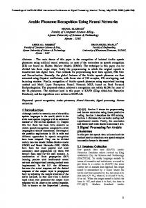
Figure 2.1: A speech recognition system. waveform. Then, the most likely word sequence for the given speech feature vectors is found using two types of knowledge sources, i.e., acoustic knowledge and linguistic knowledge. The HMM is used to capture the acoustic features of speech sound and the stochastic language model is used to represent linguistic knowledge. In this chapter,
9
each component of the block diagram is explained in detail.
2.1 Feature Extraction As air is expelled from lungs, tensed vocal cords are caused to vibrate by the air flow. These quasi-periodic pulses are then filtered when passing through the vocal tract and the nasal tract, producing voiced sounds [20]. The different positions of articulators, such as jaw, tongue, lips, and velum, produce different sounds. When vocal cords are relaxed, the air flow either passes through a constriction in the vocal tract or builds up pressure behind a closure point and the pressure is suddenly released, causing unvoiced sounds [20]. The positions of constriction or closure decide different sounds. Speech is simply a sequence of these voiced and unvoiced sounds, which vary slowly (5 100 ms) because the configuration of the articulators changes slowly. Figure 2.2 (a) shows an example of a speech waveform of the sentence, “She had your dark suit”, spoken by a male speaker. For automatic speech recognition by computers, feature vectors are extracted from speech waveforms. A feature vector is usually computed from a window of speech signals (20 30 ms) in every short time interval (about 10 ms). An utterance is represented as a sequence of these feature vectors. A cepstrum [14][76] is a widely used feature vector for speech recognition. The cepstrum is defined as an inverse Fourier transformation of a logarithmic short-time spectrum. Lower order cepstral coefficients represent the vocal tract impulse response. In an effort to take auditory characteristics into consideration, the weighted averages of spectral values on logarithmic frequency scale are used instead of magnitude spectrum, producing mel-frequency cepstral coefficients (MFCC) [17]. The time derivatives of the MFCC are usually appended to capture the dynamics of speech. See Section 5.2.1 for the detail of feature extraction procedure. Figures 2.2 (b) and (c) are the spectrogram and MFCC extracted from the example utterance.
10
(a) Waveform. 4
x 10
Amplitude
1
0 she −1 0
had 0.1
your 0.2
0.3
dark 0.4 0.5 Time (seconds)
suit 0.6
0.7
0.8
0.6
0.7
0.8
0.7
0.8
(b) Spectrogram. Frequency (Hz)
8000 6000 4000 2000 0 0
0.1
0.2
0.3
0.4 0.5 Time (seconds)
Dimension
(c) Feature vectors (cepstra).
0
0.1
0.2
0.3
0.4 0.5 Time (seconds)
0.6
Figure 2.2: An example of speech waveform, spectrogram, and feature vectors. One popular technique for robust speech recognition, which is applied to cepstral coefficients, is cepstral mean normalization (CMN) [2][25]. Since convolutional distortions such as reverberation and different microphones become additive offsets after taking the logarithm, subtracting the noise component from distorted speech will provide the clean speech component. However, estimating convolutional noise from distorted speech is not an easy task. The CMN approximates the convolutional noise component with the mean of cepstra, assuming that the average of the linear speech spectra is equal to 1, which is obviously not true. The mean vector of each utterance is computed and subtracted from the speech vectors. It has been observed that the CMN produces robust features for the convolutional noise case (see Section 5.3.3). Although
11
the CMN is simple and fast, its effectiveness is limited to the convolutional noise because it removes the spectral tilt caused by the convolutional noise. Also, estimating the mean vector is not reliable when an utterance is too short.
2.2 Hidden Markov Models Speech recognition can be considered as a pattern recognition problem. If the distribution of speech data is known, a Bayesian classifier,
U = arg Umax P (U jX ) � 2U
(2.1)
finds the most probable utterance U (word sequence), for the given feature vectors X (observation sequence). Bayesian classifiers are optimal in a sense that the probability of error is minimum [19][24]. An HMM [81] can be considered as a special case of the Bayesian classifier. In this section, how speech is represented by an HMM is discussed.
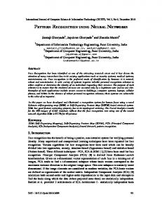
2.2.1 Acoustic Modeling One of the distinguishing characteristics of speech is that it is dynamic. Even within a small segment such as a phone1 , the speech sound changes gradually. The beginning of a phone is affected by the previous phones, the middle portion of the phone is generally stable, and the end is affected by the following phones. The temporal information of speech feature vectors plays an important role in recognition process. In order to capture the dynamic characteristics of speech within the framework of the Bayesian classifier, certain temporal restrictions should be imposed. A 3-state left-to-right HMM is usually used to represent a phone. Figure 2.3 shows an example of such an HMM, where ai j represents a state transition probability from the state i to the state j , and bi (x) is the observation probability of the feature vector x given the state i. Each state in an HMM 1 A phone is realization of a phoneme; i.e., the physical sound produced when a phoneme is articulated.
A phoneme is the smallest meaningful contrastive unit in the phonology of a language.
12
a 1,1
a
,1
1
a 1,2
a 2,2
2
a 3,3
a 2,3
3
a 3,
Entry
Exit b1 (x)
b2 (x)
b3 (x)
Figure 2.3: 3-state left-to-right HMM. models the distribution of a sound in a phone. The phone HMM in Figure 2.3 consists of 3 consecutive distributions. A word HMM can be constructed as a concatenation of phone HMM’s. A sentence HMM can be made by connecting word HMM’s. The probability of speech feature vectors generated from an HMM is computed using the transition probabilities between states and the observation probabilities of feature vectors given states. For example, consider an observation sequence consisting of seven vectors; X
= x(1)x(2) � � � x(7), where x(t) denotes a feature vector at time t in the
sequence. Suppose that the first two vectors belong to the first state, the next three vectors belong to the second state, and the rest belong to the last state. The probability of the observation sequence X and this state assignment S , given the utterance HMM U , can be computed as follows;
P (X� S jU ) = a2 1b1(x(1))a1 1b1(x(2)) � a1 2b2(x(3))a2 2b2(x(4))a2 2b2(x(5)) � a2 3b3(x(6))a3 3b3(x(7))a3 2 �
(2.2)
where ai j is the state transition probability, and bi (x(t)) is the observation probability of the feature vector x(t) given the state i. To compute the probability of the observation sequence X given the HMM U , all conditional probabilities of X and S given U have to be summed over all possible state/vector assignments (also called state/frame
13
alignment);
P (X jU ) =
X S 2S
P (X� S jU ) �
(2.3)
where S � is all possible state sequences. This summation takes O(js� jjX j) time in general, where
js�j is the number of states in an HMM and jX j is the number of feature
vectors. There exists a more efficient algorithm that takes polynomial time, which will be discussed in Section 2.3.
2.2.2 Sub-word Modeling In large vocabulary speech recognition (LVCSR), it is difficult to reliably estimate the parameters of all the word HMM’s in the vocabulary because most of the words do not occur frequently enough in training data. Furthermore, some of vocabulary words may not even be seen in the training data, which degrades recognition accuracy [52]. On the other hand, the number of sub-word units such as phones are usually smaller than the number of words. Most languages have about 50 phones. There are more data per phone model than per word model, and all phones occur fairly often in a reasonable size training data [55]. A monophone HMM models one phone. It is a context-independent unit in the sense that it does not distinguish its neighboring phonetic context. In fluently spoken speech, however, a phone is strongly affected by its neighboring phones, producing different sound depending on the phonetic context. This is called the coarticulation effect. It is due to the fact that the articulators can not move instantaneously from one position to another. In order to handle the coarticulation effect more effectively, context-dependent units [4][55][92] such as biphones or triphones can be used. A biphone HMM models a phone with its left or right context. A triphone HMM represents a phone with its left and right context. For example, the sentence “She had your dark suit” can be represented as
R
i h æ d j u @r d a r k s u t
14
using monophones. The same sentence can be represented as
�-R-i R-i-� �-h-æ h-æ-d æ-d-� �-j-u j-u-@r u-@r-� �-d-a d-a-r a-r-k r-k-� �-s-u s-u-t u-t-� using triphone models. In continuously spoken speech, the pronunciation of the current word is affected by its neighboring words. A cross-word triphone HMM handles this coarticulation effect between words. When cross-word triphones are used, the example sentence is represented as
�-R-i R-i-h i-h-æ h-æ-d æ-d-j d-j-u j-u-@r u-@r-d @r-d-a d-a-r a-r-k r-k-s k-s-u s-u-t u-t-� : The more detailed context-dependent units are used, the larger the number of units grows. The number of triphones may become larger than the number of vocabulary words. This gives rise to the trainability problem again; i.e., not enough data per model. This problem is handled by merging similar context models together. The merging can be done at the phone level or at the state level [43][55][107][106]. In any case, an HMM requires a large amount of training data to reliably estimate the parameters. Even though the parameter estimation procedure is computationally efficient, collecting the training data is a very expensive task. For a new or unknown environment, retraining or multistyle training is expensive in terms of data collection. In these cases, approaches such as parameter adaptation discussed in Section 2.3.2 are more desirable.
2.2.3 Assumptions of Acoustic Modeling The acoustic modeling of automatic speech recognition has some limitations. The use of MFCC as a feature vector, and the HMM that employs Gaussian distribution as a phone model are based upon the following assumptions.
�
Speech is assumed to be stationary during a short period of time (10 30 ms). A feature vector is usually computed from this stationary period of speech signals.
15
�
A Gaussian distribution is usually used to represent the distribution in a state. This means that the speech is assumed to be Gaussian. That is, the random deviation of a speech sound in a state follows Gaussian distribution.
�
In order to simplify the probability computation, each dimension of the speech feature vector is assumed to be independent. This assumption leads to diagonal covariance matrices, and speed-up in the computation.
�
As can be seen in the following sections, the algorithms for parameter estimation and speech recognition assume that the likelihood of a state depends on its previous state only. That is, it is assumed to be first-order dependent.
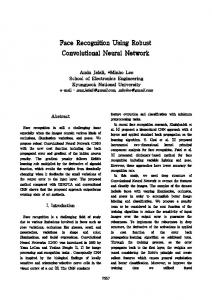
Speech is not first-order dependent. Nor is it normally distributed. Usually, a mixture of Gaussian distributions is used to represent a state in an HMM. As can be seen in the next section, the parameters of each distribution is estimated from training data. Statistical pattern recognition approaches may fail, if the estimated parameters misrepresent the true population. Figure 2.4 shows the distributions of the sound “b”. Only the first dimension of the feature vector in the middle state of a triphone model (see Section 2.2.2) of which the base phone is “b” is shown. The distorted speech is noisy distant-talking speech (see Section 5.1.4 for how the distorted speech is recorded). Because of the interference from environments as discussed in Section 1.1, the same segment of “b” sound shows different empirical distributions. Figure 2.5 shows the distribution of the same speech segment after the CMN processing. As seen in this figure, the CMN aligns the mean of the two distributions. Even though word recognition accuracies go down after the CMN, it changes the shape of distributions. For example, the bimodal distribution in Figure 2.4 (a) becomes unimodal in Figure 2.5 (b) after the CMN processing.
16
(a) Clean speech distribution.
P(x|s)
0.2
0.1
0 −40
−30
−20
−10 0 10 First cepstral coefficient
20
30
40
20
30
40
30
40
30
40
(b) Distorted speech distribution.
P(x|s)
0.2
0.1
0 −40
−30
−20
−10 0 10 First cepstral coefficient
Figure 2.4: Empirical distributions of sound “b”. (a) Clean speech distribution (after CMN).
P(x|s)
0.2
0.1
0 −40
−30
−20
−10 0 10 First cepstral coefficient
20
(b) Distorted speech distribution (after CMN).
P(x|s)
0.2
0.1
0 −40
−30
−20
−10 0 10 First cepstral coefficient
20
Figure 2.5: Empirical distributions of sound “b” after the CMN processing.
17
2.3 HMM Parameter Estimation The distribution of each state is estimated from training data. Once the association of each vector of training examples to its corresponding state is determined, the usual sample mean and sample covariance estimation techniques can be used for the parameter estimation. However, this association is not known in advance. There is no known method to analytically solve for the parameter set that maximizes the probability of training examples in a closed form. However, by iteratively applying the expectation maximization (EM) algorithm [18] (also known as Baum-Welch algorithm for HMM), a locally maximized parameter set can be found numerically [9][10][11][47][59][82].
2.3.1 Expectation Maximization Let U represent an HMM and U be an updated version of U . The EM algorithm finds a new parameter set for U such that the likelihood of the training data X given the new model U is increased; P (X jU ) iliary function Q,
Q(U� U ) =
� P (X jU ). This is done by maximizing Baum’s auxX
P (X� S jU ) log P (X� S jU ) �
S 2S
(2.4)
where S is a state sequence, and S� represents all possible state sequences for a given HMM. Intuitively, since the
Q function is a negative entropy, decreased randomness
will cause increased probability. It can be proven mathematically that increasing the value of the Q function leads to the increased likelihood [11]; if Q(U� U ) �
Q(U� U ),
then P (X jU ) � P (X jU ). Therefore, maximizing Q(U� U ) will result in the increased likelihood of the training data given the model.
P (X� S jU ) and log P (X� S jU ) in equation (2.4) can be expressed in terms of state transition probabilities and output probabilities defined in Section 2.2.1;
P (X� S jU ) =
Y t
as t; (
(t))
s t bs(t) (x
1) ( )
(2.5)
18
log P (X� S jU ) =
X
log as t; (
st
1) ( )
t where s(t) is the t-th state in the state sequence
+ log bs t (x(t)) �
(2.6)
( )
S (or equivalently, s(t) is the state at
time t in the state sequence S ). Note that the initial transition from an entry state and the final transition to an exit state is not shown for the simplicity of notation. When they are omitted, it should be clear from the context. Now, Q(U� U ) can be rewritten
Q(U� U ) = =
XY
as t; (
S 2S t
XY
1)
as t; (
S 2S t
XY
1)
(t) X (t) s(t) bs(t) (x ) (log as(t;1) s(t) + log bs(t) (x )) (2.7) t (t) X s(t) bs(t) (x ) log as(t;1) s(t) + t
(t) X (t) (2.8) s(t) bs(t) (x ) log bs(t) (x ) : t S 2S t Each state sequence passes through only one state at a time. Summing over the state
as t; (
1)
sequences that pass through a state at a certain time yields the probability of passing the state. Let P (X� s at tjU ) be the probability of passing through the state s at time t, and P (X� s_ at t;1jU ) be the probability of passing through state s_ and
s at time t;1
and t, respectively. Then, Q(U� U ) can be rewritten as follows using these probabilities summing over states instead of over state sequences;
XXX
Q(U� U ) =
s_
s
XX
t
P (X� s_ at t;1� s at tjU ) log as_ s +
P (X� s at tjU ) log bs (x(t)) :
(2.9) t Because the two terms in the right hand side of the equation (2.9) are independent, they
s
can be maximized separately. The reestimation formula for the state transition probability, as_ s , can be derived by taking a partial derivative and solving for it, subject to the stochastic constraint
P a = 1; s s_ s P P (X� s_ at t;1� s at tjU ) as_ s = t P P (X� s_ at t;1jU ) :
(2.10)
t
As discussed in Section 2.2.1, a mixture of Gaussian distributions is usually used to model the distribution in a state;
bs(x) =
X g
cs g q 1n e; (2�) jVs g j
1 2
;1 (x;m ) (x;ms�g )T Vs�g s�g
�
(2.11)
19 where cs g is the weight of the g -th PDF in state s, and ms g and Vs g are the g -th PDF’s mean vector and covariance matrix in the state s. Having multiple PDF’s in a state is equivalent to having multiple sub-states in parallel with one PDF per sub-state. The PDF’s weight, cs g , can be considered as the state transition probability into the g -th sub-state in the state s. With this interpretation, the second term in equation (2.9) can be written as follows for the Gaussian mixture case;
XX s
P (X� s at tjU ) log bs (x(t)) t XXX = P (X� s at t� PDF=gjU ) log bs g (x(t)) s
=
t
g
XXX s
t
g
(2.12)
P (X� s at t� PDF=gjU ) log cs g ; 12 log(2�)n ;
1 log jV j ; 1 (x ; m )T V ;1(x ; m )� � sg sg sg sg 2 2
(2.13)
where bs g (x(t)) is the likelihood of feature vector x(t), given the g -th PDF of state s. Since a PDF’s weight can be considered as a state transition probability into a sub-state, its reestimation formula can be derived in a similar way as in equation (2.10);
cs g
P P (X� s at t� PDF=gjU ) : = t P P (X� s at tjU ) t
(2.14)
By taking the partial derivatives and equating to zero, equation (2.13) can be maximized. This leads to the following reestimation formulae for mean vectors and covariance matrices;
ms g Vsg
P P (X� s at t� PDF=gjU )x(t) = t P P (X� s at tjU ) t P P (X� s at t� PDF=gjU )(x(t) ; m )(x(t) ; m )T sg = t : P P (X� s at tjU ) s g t
(2.15) (2.16)
Equations (2.10) and (2.14) are the weighted averages of state transitions. Equations (2.15) and (2.16) are the weighted sample mean and sample covariance estimation. To explain how to compute these values efficiently, some more variables need to be defined. Let �(st) be the probability of the partial observation sequence, x(1)x(2) � � � x(t),
20 and state s at time t, given the model U (also called forward probability);
�(st) = P (x(1)x(2) � � � x(t)� s at tjU ) :
(2.17)
It represents the likelihood of a partial sequence at a state; i.e., how likely it is for the partial sequence to reach the state. It can be computed recursively;
X
�(st+1) =
s_
�(s_t)as_ sbs(x(t+1))
(1) �(1) s = a2 s bs (x ) �
(2.18) (2.19)
where as_ s is equal to 0 if there is no connection between the states s_ and s. The likeli-
X = x(1)x(2) � � � x(T ), given the model U can be expressed as the forward probabilities at time T and the state transition proba-
hood of the complete observation sequence,
bilities to the exit state;
P (X jU ) = Similarly, let
�s(t)
X s
�(sT )as 2 :
(2.20)
be the probability of the partial observation sequence,
x(t+1)x(t+2) � � � x(T ), given state s at time t and model U (also called backward probability);
�s(t) = P (x(t+1)x(t+2) � � � x(T )js at t� U ) :
(2.21)
It represents the probability that the rest of the observation sequence,
x(t+1)x(t+2) � � � x(T ), is produced by the model U starting from state s at time t. It can be computed recursively as well;
�s(t) =
X s_
as s_ bs_ (x(t+1))�s(_t+1)
�s(T ) = as 2 : The likelihood of the complete observation sequence
(2.22) (2.23)
X , given the model U , can be
computed using backward probabilities as well;
P (X jU ) =
X s
a2 sbs(x(1))�s(1) :
(2.24)
21 The computation of �(st) and �s(t) for all states and times can be done in O(js� j2
� jX j)
time using dynamic programming, where js�j is the number of states and jX j is the number of vectors. Finally, let �s(t) be the probability of being in state s at time t, given the observation sequence
X and the model U (also called state occupying probability or simply state
occupancy);
�s(t) = P (s at tjX� U ) s at tjU ) = P (X� P (X jU ) s at tjU ) = PP P(X� s (X� s at tjU ) (t) (t) = P�s (�t)s (t) : s �s �s
(2.25) (2.26) (2.27) (2.28)
Equation (2.28) is derived from the fact that the probability of passing through state s at time t is equivalent to �(st)�s(t), and summing it over all states yields the likelihood of the observation sequence given the model. Similarly, let �s(tg) be the probability of being in the g -th PDF of state s at time t,
given the observation sequence X and model U ;
�s(tg) = P (s at t� PDF=gjX� U ) (2.29) (t) = g jU ) = �s(t) P (x P (� xs(att)� t�s PDF (2.30) at tjU ) (t) = �s(t) bbs g((xx(t))) � (2.31) s where bs g (x(t)) is the probability of observation vector x(t) and g -th PDF, given state s. Note that the probability of the observation going through from state s_ to s at time t ; 1 and t, given the model U , i.e., P (X� s_ at t;1� s at tjU ), is equivalent to �(s_t;1)as_ sbs(x(t))�s(t). The probability of passing through state s at time t;1, given the model U , i.e., P (X� s at t;1), is �(st;1) �s(t;1). The probability of the observation passing through g -th PDF of the state s at time t, given the model U , i.e., P (X� s at t� PDF=
22
gjU ), is �(st)�s(t) bbs�gs((xxtt)) . ( )
( )
Now, the reestimation formula can be expressed in terms of
these new variables;
as_ s
P �(t;1)a b (x(t))� (t) = t Ps_ (t;s_ s1) s (t;1) s � �
(2.32)
t s_
cs g =
s_ P �(t)� (t) bs�g (x(t)) t s s bi (x(t) ) P �(t)� (t) t s s
(2.33)
ms g
P �(t)� (t) bs�g (x t ) x(t) t t = P s (t)s (tb)ib(s�gx (x) t ) � �
Vsg
P �(t)� (t) bs�g (x t ) (x(t) ; m )(x(t) ; m )T sg sg t s s bs (x t ) : = P �(t)� (t) bs�g (x t )
( )
( )
t s
(2.34)
( )
s bs (x(t)) ( )
By
( )
t s
normalizing
both
numerators
( )
s bs(x(t) )
and
denominators
with
(2.35)
P �(t)� (t), s s s
equation (2.33) (2.35) can be further simplified as follows;
cs g ms g Vsg
P � (t) = Pt s(tg) t �s P � (t)x(t) t sg = P (t) t �s g P � (t)(x(t) ; m )(x(t) ; m )T sg sg : = t sg P � (t) t sg
Since both �(st) and �s(t) can be computed in O(js�j2
(2.36)
(2.37)
(2.38)
� jX j) time, �s(t) also can be com-
O(js�j2 � jX j) time. Therefore, one iteration of the parameter reestimation procedure can be done in O(js� j2 � jX j) time. puted in
To reliably estimate the parameters of HMM’s, a large amount of training data is required. For example in [50][64][78][105], hundreds of hours of speech data is used for training. More training data always decreases recognition error rates. However, the improvement curve follows logarithmic growth. Collecting a large amount of training data is an expensive task in terms of human effort. For a new environment, therefore, a speech recognizer trained on already existing clean speech corpora are usually adapted to the new environment using a small amount of environment specific data
23
[30][32][58][90]. One of these parameter adaptation methods is discussed in the next section.
2.3.2 Parameter Adaptation The maximum likelihood linear regression (MLLR) [57] is a speaker adaptation method for continuous density Gaussian mixture HMM’s. It has been recently applied to robust speech recognition where recognizers are adapted to a new environment instead of a new speaker [103]. The MLLR estimates a set of transformation matrices for model parameters, i.e. means and variances of Gaussian mixtures. The transformation matrices are estimated in such a way that the transformed models maximize the likelihood of the adaptation data. In this section, a mean transformation MLLR [57] is described. The MLLR assumes that an adapted mean vector can be represented as an affine transformation of the original mean vector;
ms g = Am^ s g �
(2.39)
where ms g is the adapted mean, A is an n+1 by n transformation matrix that MLLR estimates, and m ^ s g is an n+1 dimensional vector that is composed of the original mean vector and an additional dimension of some constant value. This is to accommodate an affine transformation in a single matrix multiplication. The output probability of the adapted model becomes
bs(x) =
X g
1 e; n (2�) jVs g j
cs g q
1 2
;1 (x;Am (x;Am^ s�g )T Vs�g ^ s�g )
The likelihood of adaptation data can be increased by maximizing
:
(2.40)
Q(U� U ).
Taking
derivatives of Q(U� U ) with respect to the transformation matrix A, and equating it to zero leads to the following condition;
XX t
g
�s(tg)Vs;g1 x(t)m^ Ts g =
XX t
g
�s(tg)Vs;g1Am^ s gm^ Ts g :
(2.41)
24 By solving equation (2.41) for the transformation matrix A in a diagonal covariance case, the reestimation formula for A can be derived as follows;
Ar = BC ;1(r) X X (t) ;1 (t) T B = �s g Vs g x m^ s g t
Ck l(r) =
g
XX g
t
where Ar is the r-th row of the matrix A,
�s(tg)vr;1m^ s g k m^ Ts g l �
(2.42) (2.43) (2.44)
Ck l(r) is the k-th row l-th column element
of matrix C (r). When there are enough adaptation data, one transformation matrix may be estimated for each mean vector. At the other extreme, when only a small amount of adaptation data is available, all models may share one transformation matrix. The MLLR is effective for the case where the distortion process can be modeled as an affine transformation (or a set of affine transformations). It is especially effective compared to MAPbased method [32] when there is a small amount of adaptation data available (see Section 5.4.6). This is because the number of parameters that has to be estimated is much smaller in the MLLR case than in the MAP case. However, the MLLR is not useful for the distortion that can not be modeled by an affine transformation, such as additive noise or multiply distorted speech (see Section 5.3.3). Moreover, it is not appropriate for variance transformation which is seldom modeled as an affine transformation. As is the case of all EM algorithms, the parameter reestimation procedure heavily depends on an initial parameter set. If the initial parameter set is quite different from the distribution of adaptation data as in Figure 2.5, it often converges to a local maximum.
2.4 Decoding Algorithms Depending on the type of speech recognition unit, automatic speech recognition can be divided into two groups; isolated word recognition and continuous speech recognition. The isolated word recognition assumes that a word is uttered in a discrete manner so
25
that there are silences at the beginning and the end of each word. The continuous speech recognition is more difficult and complicated compared to the isolated word recognition because word boundaries are not known and are often ambiguous.
2.4.1 Isolated Word Recognition In isolated word recognition, a word can be represented by a word HMM, or by the concatenation of phone HMM’s. A testing speech, X , is classified as one of the vocabulary words, W , according to the following Bayesian framework;
W = arg Wmax P (W jX ) 2W
(2.45)
P (X jW )P (W ) = arg Wmax 2W P (X )
(2.46)
� arg Wmax P (X jW ) � 2W
(2.47)
where W � represents all the vocabulary words. Since the denominator, P (X ), is common to all words, it can be simply discarded. Assuming that all words are equally
P (W ), can also be dropped. P (X jW ) is the likelihood of the testing utterance X , given the word model W . It can be computed usprobable, the prior probability,
ing equation (2.20) or (2.24). The total execution time to find the most probable word is
O(jW �j � js�j2 � jX j) because the likelihood has to be computed for each word.
Whichever word has the highest probability is recognized as the uttered word.
2.4.2 Continuous Speech Recognition Depending on the type of grammar for language models in continuous speech recognition, it can be as simple and constrained as command recognition or digit string recognition [82], and as sophisticated and unconstrained as dictation of naturally spoken speech [96]. The command or digit string recognition usually makes use of finite state grammars. The unconstrained dictation systems typically use statistical language models
26 such as n-gram [49]. In this section, the large vocabulary continuous speech recognition that uses a statistical language model is explained. Theoretically, continuous speech recognition is accomplished by finding the utterance, U , which gives the highest probability for the given observation sequence X ;
U = arg Umax P (U jX ) 2U
(2.48)
P (X jU )P (U ) = arg Umax 2U P (X )
(2.49)
= arg Umax P (X jU )P (U ) � 2U
(2.50)
where U � is all the possible utterances (word sequences), P (X jU ) is the likelihood of the observation sequence X for the given utterance U , and P (U ) is the a priori probability of the utterance U . Since the denominator P (X ) is common to all utterances, it can be discarded as in Section 2.4.1. The acoustic model score, puted using an utterance HMM. The language model score,
P (X jU ), is com-
P (U ), is computed using
stochastic language model such as bigram or trigram [49];
P (U ) =
� �
Y i
Y i
Y i
P (Wi jW1� W2� � � � � Wi;1)
(2.51)
P (Wi jWi;2� Wi;1)
(trigram)
P (Wi jWi;1)
(bigram)
(2.52)
:
(2.53)
A bigram is a probability of a word given one previous word. A trigram is a probability of a word given two previous words. These n-gram probabilities are used to approximate the original conditional probability, i.e., equation (2.51), which is computationally intractable. The n-gram language models are usually built using co-occurrence information from a large amount of text data, typically consists of hundreds of millions of words [50][105]. The direct application of equation (2.50) is not feasible because there exist too many possible utterances even for a small size vocabulary; i.e., exponentially many word sequences to test. Instead of testing each utterance separately, one generic speech model is
27
built to represent all possible utterances. Then, the best word sequence is approximately computed from the best state sequence of the testing speech given the generic model [54]. Figure 2.6 shows the structure of the generic speech model. It is built by con-
W1
W2 Entry
Exit
Bigrams
Wn Word models
Optional silences
Figure 2.6: Generic utterance HMM. necting word HMM’s in parallel. Each word HMM can be made of sub-word HMM’s as discussed earlier. In this figure, each word can jump to any word in the vocabulary. Between words, there may be a short silence. This silence is absorbed by an optional silence model that has a skip transition; i.e., the transition from entry to exit without going through an actual state. When the bigram is used as a language model, the path from Wj to Wi has the bigram probability P (Wi jWj ). This bigram probability can be viewed as a state transition probability from the exit state of Wj to the entry state of
Wi. This composite model is nothing but a complex structure HMM which can represent arbitrary word sequences. The best state sequence for a testing speech given this generic model can be found using the Viterbi algorithm [22][100]. The essence of the Viterbi algorithm is the following observation. Suppose that the best path to state s at
time t is through state s_ at time t;1. Then, the global best path to the state s is composed of the local best path to the state s_ and the path from state
s_ to s.
This is because the
path score is only first-order dependent. Previous history in a path does not affect the
28
current transition probability. Therefore, only the local best path coming to the current state from one previous state needs to be maintained. At the end of the utterance, the global best path can be found by backtracking the local best path;
� (t;1)a b (x(t)) �s(t) = max � s_ s s s_ s_
(2.54)
�s(t) = arg max �(t;1)as_ s � s_ s_ where �s(t) is the probability of the local best path to state
(2.55)
s at time t, and �s(t) is the
previous state in the local best path to state s at time t. The computation of the Viterbi path is illustrated in Figure 2.7. At time t, each state has to check all incoming paths to
State
Time 1
1
1
1
1
1
1
2
2
2
2
2
2
2
3
3
3
3
3
3
3
Figure 2.7: Viterbi path computation. find the best one. It takes O(js�j2
� jX j) time to compute the Viterbi path, and O(jX j)
to trace it back. Once the best state sequence is found, its corresponding word sequence can be constructed because a state can belong to only one word. This word sequence computed from the Viterbi path is suboptimal. Instead of the likelihood of an utterance, only one best path score is used to find the most likely utterance;
P (X jU ) =
X
S 2S
P (X� S jU )
� max P (X� S jU ) : S 2S
(2.56) (2.57)
Nevertheless, the Viterbi algorithm produces good recognition results [8], because the best path score is usually a dominant factor of the likelihood computed from an HMM.
29
This approach for continuous speech recognition, however, is applicable when it is based on the bigram language model. If the trigram model is used, the bigram transition probabilities in Figure 2.6 can no longer be used, because the trigram is second-order dependent. The generic utterance HMM becomes too complex to incorporate trigrams. In general, for an n-th order dependent language model, the generic HMM becomes a tree with height n, where each node in the tree represents a word model and has all the words in the vocabulary as its children. The Viterbi algorithm is exponential with respect to the order of the language model. In large vocabulary continuous speech recognition, higher order n-grams play an important role. However, using more complex model than a bigram is computationally expensive, especially when the size of vocabulary is large. In the n-best decoding approach [71][91], a lower order n-gram is used to generate a set of likely utterance hypotheses. Then, the hypotheses are reordered using more complex acoustic models and a higher order language model. The best hypothesis in the reordered list is chosen as the recognized sequence of words . The n best hypotheses can be found in polynomial time using the tree-trellis search algorithm [94] which is a combination of Viterbi algorithm and A� algorithm [37][38][72]. In the stack decoding approach [35][46][79], the breadth first characteristic of the Viterbi search is changed to depth first. The most promising partial hypothesis is explored first. If it is found to be not likely later, another partial hypothesis with possibly different time and length is explored. The backtracking scheme is implemented using a stack. Choosing the most promising partial hypothesis depends on local lookahead information [6] or some heuristic functions [79]. The word graph decoder [3] first produces a word graph using a lower order n-gram. The word graph is a directed acyclic graph (DAG) where each edge is associated with a word and each vertex is associated with a time mark [75]. It is an efficient representation of alternative hypotheses for an utterance. A word graph has usually fewer words in it than the original vocabulary. The higher order language model can be used in the second pass of decoding with a restricted set of words and their
30
transitions defined by the word graph produced in the first pass. In fact, this can be repeated progressively each time using more sophisticated language and acoustic models to generate smaller word graphs [69]. The word graph approach is basically a variation of the n-best approach, where a word graph is used instead of an n-best hypothesis list. Recently, an efficient representation of a dictionary using a tree structure [70], and an efficient implementation of a higher order Viterbi algorithm makes it possible to do one pass decoding for a large vocabulary [74][112]. In this approach, the unlikely partial hypotheses are pruned, and only the likely partial hypotheses are maintained dynamically. Unlike the stack decoder, all the likely partial hypotheses are explored synchronously. The number of partial hypotheses easily becomes intractable. The key to the success of this approach is how to maintain a relatively small number of partial hypotheses and still produce reliable results.
2.5 Summary In this chapter, the fundamentals of automatic speech recognition algorithms have been explained. Automatic speech recognition can be considered as a statistical pattern recognition problem. The most commonly used feature vector for speech recognition is the cepstrum. It represents the shape of the spectral envelope of the speech during a short time interval. The HMM is used for the acoustic models, and the n-gram is used for the language models. The Viterbi algorithm integrates these two components under the Bayesian framework, and finds the most likely utterance for a given speech. However, this statistical approach may fail if the training and the testing data distributions are different. In the next chapter, the neural network based transformation methods that address this problem are discussed.
31
Chapter 3 Adaptation Using Neural Networks In order to handle the mismatch between training and testing environments, many techniques have been proposed. Some methods work on feature vectors [1][2][25], while others work on the parameters of a recognizer, either without assuming any prior knowledge about the mismatching environments [32][53], or with assumptions such as obtainability of linear spectra from cepstra[28][29][30] or linearity of the underlying distortion functions [26][27][57][58][90]. In general, the less assumptions used, the more adaptation data is required. In this chapter, a neural network based adaptation approach is explored, which does not assume any linearity of the mismatching environments, while maintaining the amount of adaptation data small. First, the computability and training algorithm for a neural network are discussed. Then, the neural network is applied to the feature vector transformation to handle the training and testing environment mismatches.
3.1 Multi-Layer Perceptrons Neural networks have been used in many aspects of speech recognition. They have been used as phoneme classifiers [101][108], isolated word recognizers [51], and probability estimators for speech recognizers [15][68][85][87]. In this section, one of the most popular type of neural networks, multi-layer perceptrons (MLP), is briefly described. Some of the theory and a tutorial on MLP can be found in [60][89], and a survey of applications to speech and other areas can be found in [42][61].
32
3.1.1 Perceptrons A perceptron [88] models a neuron in a brain. Its output is defined as 1 if the weighted summation of its inputs is greater than some threshold value, and 0 otherwise. Figure 3.1 shows a perceptron. The input is represented as x_i , and the corresponding weight
Output
w1 w2 .
x1
wn
.
Weights .
x n Input
x2
Figure 3.1: A perceptron. is represented as wi . The threshold can be considered as an extra weight for which the input is always 1. The output of a perceptron is then,
output
8 > :0
P w x_ > 0 i i otherwise : if
(3.1)
This simple computational model can be considered as a two-class classifier; it outputs 1 for one class and 0 for the other. The learning in a perceptron involves adjusting the weights
wi.
It can be viewed that a perceptron represents a hyper-plane in a
n-dimensional space. This hyper-plane separates (classifies) all the vectors that lie on one side from the others. The equation for this decision surface is wT � x_ = 0. The weights are adjusted by interactively presenting training examples (pairs of input and target patterns) to the perceptron. For each training example, if the target (desired output) and the perceptron output are not same, the weights are adjusted according to the following rule;
wi wi + wi
(3.2)
33
wi = (x ; xi) x_ i �
(3.3)
where is the learning rate (also called step size) that decides the speed of convergence, and xi and xi are the i-th dimensional target value and output value, respectively. For example, if the target value is 1, the output is -1, and the input is positive, then the weight is increased. This makes sense intuitively because the increased weight will help to make the output closer to 1 than before. Rosenblatt [88] proved that the weights of a perceptron converge to some vector which classifies all the training examples correctly after a finite number of training iterations, provided that the training data are linearly separable.
3.1.2 Computability of Neural Networks A single perceptron can be used to represent a boolean function such as NOT, AND, and OR operators. However, it can not represent an XOR function [66] because a perceptron is equivalent to a line in a 2-dimensional space and the XOR function is not linearly separable. However, by using more than one layer perceptrons, every boolean function can be represented. In general the following has been proved [60]. One-layer perceptrons can handle linearly separable problems in multi-dimensional space. Two-layer perceptrons can separate any convex regions by intersecting several hyper-planes. Three-layer perceptrons can distinguish any shape of region by combining two-layer perceptrons. Figure 3.2 shows a three-layer (two hidden layers and one output layer) feed-forward neural network. See [16][33][39][40][44][97] for more on the capabilities of the multilayer perceptrons.
3.1.3 Generalized Delta Rule There is no known solution that finds an optimal weight set for a feed-forward neural network. The weights of an MLP are usually trained using an iterative hill climbing method. Instead of a hard threshold function as in Figure 3.1, a sigmoid function,
34
Output Output layer
Second hidden layer
First hidden layer
.
x1
.
x2
.
xn
Input
Figure 3.2: Two-hidden-layer perceptrons.
1 1+e;�wi x_ i , is used as an activation function of a neuron in an MLP. The error of a neural network is defined as
X E = 12 (xi ; xi)2 : i
(3.4)
It is known that the neural network that minimizes the mean squared error (MSE) in equation (3.4) is the one that is most likely correct if the target feature values are distorted by Gaussian noise [67]. This objective function allows an efficient way of implementing a training algorithm such as an error back-propagation (EBP) algorithm using the generalized delta rule [89]. The training procedure adjusts the weights of a network by moving toward the steepest direction that reduces the error E . This is the opposite direction to the derivative of the function E with respect to the weights;
wi j wi j + wi j @E
wi j = ; @w ij
(3.5) (3.6)
35 where wi j is the weight between the i-th neuron in the output layer and the j -th neuron in a hidden layer. Using the chain rule, the derivative can be rewritten as follows;
@E = @E @xi @�i @wi j @xi @�i @wi j hj � = ; | (xi{z; xi)} x| i(1{z; xi)} |{z} @E @xi
@xi @�i
(3.7) (3.8)
@�i @wi�j
where �i is the input to the sigmoid function of the i-th output neuron, i.e., �i
P w h , and h is the output value of the j -th neuron in a hidden layer. j j ij j
=
The error at a hidden layer can be derived similarly. First, the error is expressed in terms of hidden layer’s weight, wjk . Then, the derivative with respect to the weight is obtained;
2 32 77 X 666 X X 1 E = 2 66xi ; �( wi j �( wjk x_ k ))777 i 4 j | k {z } 5
(3.9)
hj
@E = @E @hj @�j @wjk @hj @�j @wjk X " @E @xi @�i # @hj @�j = i @xi @�i @hj @�j @wjk X = ;(xi ; xi)xi(1 ; xi)wi j ] hj (1 ; hj )x_ k � i
(3.10)
(3.11) (3.12)
where � is the sigmoid function and x_ k is the input to the network. This can be easily generalized to the case where there is more than one hidden layer. A gradient descent search finds a set of weights in a hyper-dimensional space of weight vectors by starting with random initial weights, then repeatedly adjusting them with a small step size. There can be many local minima in the search space. It is not guaranteed to find a global minimum by the gradient descent search. By adding a momentum term to the search as follows
w(t+1) = w(t) + w(t) + w(t;1) �
(3.13)
36
which tends to force the search to follow the previous direction it took, it may escape small local minima. Also, the amount of weight change tends to increase, thereby speeding up convergence. The error on the training set keeps decreasing as the search continues. However, after some iterations, it may over fit the training examples rather than generalizing their input and output relationship. The training process is, therefore, usually monitored using a cross validation set. The iteration of weight updating is stopped when the error,
E , is minimum on the cross validation set. In this way, over fitting the training examples is avoided. Some of cross validation techniques and experimental results on neural network and other machine learning algorithms can be found in [102].
3.2 Feature Transformation Using Mean Squared Error Criterion In this section, how an MLP may be applied to handle training and testing mismatch is described. Since an MLP is a universal approximator [40], it can be used as a transformation function between training and testing environments. One way of applying this transformation is on feature vectors. That is, given a feature vector from a testing environment, it produces an approximated feature vector for the training environment [111][115]. Figure 3.3 shows a block diagram of this approach. The neural network is trained using simultaneously collected speech data (so called stereo data) in a testing environment. During training, distorted speech feature vectors are provided to the neural network as input, and clean speech feature vectors are provided as target. Once the network is trained, it can transform the distorted speech feature vectors to those that correspond to clean speech, and can pass them to a speech recognizer. The speech recognizer trained on clean speech can be used without retraining. The input and output of the neural network are the MFCC feature vectors described in Section 2.1.
37
Adaptation Clean speech
Testing speech
Speech recognizer
Neural network
Distorted speech
Figure 3.3: Robust speech recognition using neural network and HMM’s.
3.2.1 Motivation for Using MLP Even when there is only multiplicative (convolutional) and additive noise in the testing environment, the relationship between training and testing environment in terms of MFCC feature vectors is not linear because the MFCC’s are in the logarithmic domain. The multiplicative and additive distortion means
xf = af �xf +bf � ( )
( )
( )
(3.14)
( )
where a(f ) and b(f ) are some constants, x(f ) is an observed feature value and x(f ) is clean speech feature value, both in linear frequency domain. In the logarithmic domain, the relationship becomes non-linear as follow;
log x f = log a f � x f + b f ] ( )
( )
( )
( )
# b f = log a f + log x f + a f 6= log a f + log c f � log x f : ( )
"
( )
( )
(3.15) (3.16)
( )
( )
( )
( )
(3.17)
38
b That is, the additive term inside the logarithm, a((ff)) , can not be approximated with some
constant multiplicative term outside the logarithm, log c(f ) . Besides the logarithmic op-
eration, some more operations, such as time derivative computations and the CMN processing, are usually involved in computing feature vectors. These operations make it very difficult to go back to the original linear frequency domain. Therefore, an MLP is used to establish this non-linear mapping function of MFCC’s between the testing and the training speech. Since an MLP is able to represent an arbitrary non-linear function, the neural network based transformation method can handle both linear and nonlinear mismatches such as ambient noise, reverberation, channel mismatches, and their combinations. As discussed in the previous chapter, an HMM-based speech recognizer requires a large amount of speech data to reliably estimate its parameters. The neural network based transformation approach is efficient in a sense that it requires only small amount of training data to train the network compared to the one which would be required by the HMM’s. This is because the neural network provides some constraints and allows only the likely transformations, while the direct HMM parameter estimation is unconstrained and there are more free parameters to be estimated. These can be compared to the biased learning and unbiased learning. The neural network based transformation is a biased learning in this case. See Section 5.4.6 for experimental results.
3.2.2 Effect of Contextual Information For a distant-talking speech in an enclosed environment such as a room, since it is distorted by reverberation, the neighboring feature vectors in a time sequence contain some information about the current speech frame. The reverberation of previous frames remains in the current frame, and the reverberation of the current frame affects the following frames. Even if there is no reverberation, the contextual information usually helps in distinguishing speech patterns [51][41]. Figure 3.4 shows the one-hidden-layer perceptrons with a 3-frame input window. The hidden layer is connected to one previous,
39
xn
x2
x1
Output layer
Hidden layer
Input layer
C
FC
M t-1 Previous frames
t t+1 Current frame
Following frames
Figure 3.4: One-hidden-layer neural network with contextual information. the current, and one following input vectors. The activation function of a neuron in the hidden layer is sigmoid, while the output layer makes use of linear activation functions.
3.2.3 Effect of Time Derivatives In the character recognition domain, it has been suggested to include the derivatives of the target function that the network is estimating if the information is available [93]. In this way, the network is able to approximate not only the target function but also the derivatives. As discussed in Section 2.1, in large vocabulary speech recognition, the time derivatives of feature vectors are usually appended to the original feature vectors to capture the dynamic characteristics of speech. These time derivatives can also be used as a constraint to the network during the training procedure. In this case, the error term of equation (3.4) is modified to accommodate the first and the second time derivatives
40
as follows;
X X i @xi 2 1 X @ 2xi @ 2xi 2 E = 12 (xi ; xi)2 + 12 ( @x ; @ ) + 2 ( @ 2 ; @ 2 ) � (3.18) i i @ i @ 2 xi i @xi @ 2 xi where @x @� , @� , @� 2 , and @� 2 represent the first and the second order time derivatives of the target value and the network output, respectively. This additional constraint is particularly useful when the data are sparse, because it allows the network to learn not only the mapping function itself, but also the time trajectory (see Section 5.3). It should be noted that the additional error terms are used only during training and not during testing.
3.2.4 Performance Upper Bound The model adaptation approaches, such as the MLLR or the MAP, transform model parameters to best match a current testing environment which is degraded with noise. As more data is used for these types of adaptation techniques, the adapted model tends to approach a retrained recognizer on the testing environment. The performance of most model adaptation methods are, therefore, restricted to that of retrained recognizers. In some feature transformation approaches such as described in this Chapter, however, feature vectors of distorted speech are transformed to those of clean speech. As the transformation function gets more accurate, the transformed feature vectors approach the clean speech feature vectors. Therefore, the performance upper bound of the feature transformation method is that of clean speech recognizers.
3.3 Summary In this chapter, the neural network based feature transformation approach has been discussed. The convolutional and additive noise become non-linear in the cepstral domain. Also some procedures such as time derivative computations and CMN operation make
41
it difficult to handle the noise in a linear frequency domain. Neural networks are a popular mathematical tool that can model arbitrary non-linear functions without any expert knowledge. The feature transformation neural network converts distorted speech feature vectors to those that correspond to clean speech. The theoretical performance upper bound of this type of network is better than that of model adaptation methods. However, using the MSE as the objective function for the neural network may not be appropriate in the synergistic use of neural networks and HMM’s. In the next chapter, this disadvantage is analyzed and a new objective function is proposed for the global optimization of the neural network and HMM.
42
Chapter 4 Maximum Likelihood Neural Networks As seen in the previous chapter, the feature transformation neural network is typically trained to minimize the mean squared error between the target and the network output. On the other hand, HMM-based speech recognizers are usually trained to maximize the likelihood of the training examples. The two system components in Figure 3.3, the neural network and the HMM, are therefore designed from two different objective functions. In this section, the effect of the different cost criteria of a synergistic system is discussed, and a new objective function for the neural network is proposed [110][109][114][113]. First, an anomaly of the feature transformation neural network, which makes use of the mean squared error criterion as its objective function, is analyzed. Then, the new objective function for the network is proposed to globally optimize the synergistic system under consistent cost criteria. The new objective function can be applied to either a feature transformation or a model transformation.
4.1 Motivation for A New Objective Function The error criterion of neural networks is traditionally represented by the mean squared error [89]. The neural network is trained to minimize the accumulated
E
in equa-
tion (3.4), which is the squared difference between the network output (i.e., approximated clean speech) and the corresponding target (i.e., clean speech). On the other hand, continuous speech recognition is accomplished by finding the utterance, U , which gives the highest probability for the given observation sequence X ;
U = arg Umax P (U jX ) 2U
(4.1)
43
P (X jU )P (U ) = arg Umax 2U P (X )
(4.2)
= arg Umax P (X jU )P (U ) : 2U
(4.3)
As discussed in Section 2.4.2, P (U ) is the score of the word sequence U , which is usually computed using a stochastic language model trained independently from the acous-
P (X jU ) is the acoustic score of the feature vector sequence X for the given word sequence U , It is the only term in equation (4.3) that can be affected by a feature tic models.
transformation. The acoustic score of a word sequence is the product of each individual word acoustic score. As discussed in Section 2.4.2, in continuous speech recognition, the score of the best word sequence is usually approximated by the best state sequence score using the Viterbi algorithm;
P (X jU ) � max P (X� S jU ) S 2S
(4.4)
= max P (X jS )P (S jU ) S 2S = max S 2S
Y
s2S
(4.5)
P (xjs)P (sjs_) �
(4.6)
U , P (X� S jU ) is the acoustic score coming from the state sequence S for the given utterance U . Equawhere S � is all the possible state sequences for the given utterance
tion (4.6) is a result of the first-order dependency of HMM. That is, a current score de-
P (sjs_) is the state transition score from the state s_ to the state s, where s_ is the predecessor of the state s in the state sequence S . It is determined by a state transition probability, i.e., as_ s in Section 2.2.1. Therefore, the feature transformation affects only P (xjs), which is the likelihood of the observation vector x given the state s of the utterance HMM U . As discussed in Section 2.3, this likelihood
pends on only one previous state.
is usually represented using a mixture of Gaussian distributions;
X
cs g q 1n (4.7) e; (x;ms�g )T Vs�g; (x;ms�g ) � g (2�) jVs g j where cs g is the g -th distribution weight, and ms g and Vs g are the g -th distribution mean vector and covariance matrix of state s, respectively. The feature transformation using a P (xjs) =
1 2
1
44
neural network minimizes the mean squared error of equation (3.4), which does not not necessarily maximize the acoustic score P (xjs) of equation (4.7). The anomaly comes from the two different cost criteria of the synergistic system. Figure 4.1 shows an example of the inadequacy of mean squared error criterion in
x is a clean speech feature value, x1 x3 are the network output. Let us assume that the clean speech x belongs to the state s that follows the empirical distribution P (xjs). m is the mean value of this distribution. In this figure, the smaller mean squared error output, x1, is less likely than the larger mean squared error output, x2 or x3. In the next section, a new objective function for the neural network one-dimensional feature space.
x3 m
P(x|s)
0.4 0.3
x2 − x
0.2
x1
0.1 0 −5
−4
−3
−2
−1
0 1 Cepstral value
2
3
4
5
Figure 4.1: An example of MSE anomaly. x is clean speech. x1 x3 are network output. is proposed, which can handle the anomaly discussed in this section.
4.2 Feature Transformation Using MLNN One way to increase the probability in equation (4.7) is to train a feature transformation neural network to maximize it, i.e., to force the network to produce a value close to the mean of the corresponding distribution. The probability density function of equation (4.7) can be directly used as an objective function for the neural network. The conditional probability of each state is maximized by the neural network. Schematically, it replaces the clean speech target values in the original MSE neural network with HMM parameters which come from continuous density HMM’s, as shown in Figure 4.2. Since
45
Adaptation HMM parameters
Testing speech
Neural network
Speech recognizer
Distorted speech
Figure 4.2: Feature transformation MLNN. this neural network maximizes the output probability of each state, and eventually maximizes the likelihood of the observation for the given HMM’s, it will be called a maximum likelihood neural network (MLNN). The MLNN is a neural network which takes a probability distribution, not a vector, as its target. It should be noted that the MLNN can take not only Gaussian distributions, but also any differentiable probability density function as its target distribution. Therefore, the MLNN is no longer constrained to the stereo data availability. The error back-propagation algorithm [89] can still be used with the new objective function. In this section, the weight update rule for the new objective function is derived.
4.2.1 MLNN Training Algorithm A weight update rule can be derived by differentiating the equation (4.7) with respect to weight wi j (the connecting weight between output node i and hidden node j ). Since the goal is to maximize the objective function rather than to minimize it, the weight update rule makes the network move toward the direction of the derivatives instead of the opposite direction;
wi j wi j + wi j
(4.8)
46
wi j = @P@w(xjs) ij
(4.9)
As in Section 3.1.3, using the chain rule, the @P@w(xi�jjs) can be derived as follows;
@P (xjs) = @P (xjs) @xi @�i � (4.10) @wi j @xi @�i @wi j where xi is the value of the i-th output node. The first term corresponds to the error at the
output layer in the original error back-propagation algorithm with mean squared error as its objective function. The second and the third terms are the same as in the original error back-propagation algorithm (see equation (3.8) for comparison). As discussed in Chapter 2, a mixture of Gaussian distributions with diagonal covariance matrices is used to model P (xjs);
P (xjs) =
X g
1
e cg q n Q (2�) i vs g i
; 12
P
i
x;ms�g�i )2 vs�g�i
(
:
(4.11)
In this case, the first term of equation (4.10) becomes
@P (xjs) = X P (xjs� g) ms g i ; xi � (4.12) @xi vs g i g where ms g i and vs g i are the i-th dimension mean and variance of the g -th PDF in state s, respectively, and P (xjs� g) is the likelihood of the observation vector x given the g-th PDF of state s; P x;ms�g�i P (xjs� g) = cg q n1Q e; i vs�g�i � (4.13) (2�) i vs g i In a high dimensional case, P (xjs� g ) can be extremely small, often beyond the float1 2
(
)2
ing point precision of a digital computer. This problem can be solved by taking the logarithm before differentiation. The modified weight update rule is, then, derived by differentiating the logarithm of equation (4.7) with respect to weight wi j ;
@ ln P (xjs) = @ ln P (xjs) @xi @�i � @wi j @xi @�i @wi j
(4.14)
where the second and third terms are the same as in equation (4.10). The first term can be rewritten as follows for a diagonal covariance matrix case;
@ ln P (xjs) = X P (xjs� g) ms g i ; xi : @xi vs g i g P (xjs)
(4.15)
47 Compared to equation (4.12), the weighting factor P (xjs� g ) is normalized by P (xjs). This can be implemented with a subtraction operation in the logarithmic domain without the danger of precision underflow. The second and the third terms of equation (4.14) can be derived in the same way as in Section 3.1.3. The modified weight update rule for the weight wi j at the output layer becomes
wi j wi j + wi j P (xjs)
wi j = @ ln@w ij " # @ ln P (xjs) = X P (xjs� g) ms g i ; xi x (1 ; x )h : i i j @wi j P (xjs) vs g i g
(4.16) (4.17) (4.18)
The derivatives with respect to hidden layer’s weights can be derived by first expressing the likelihood P (xjs) in terms of hidden layer’s weights, and then by taking the derivatives;
wj k wj k + wj k P (xjs)
wj k = @ ln@w jk P X 1 ; q ln P (xjs) = ln cg e i g (2�)n Qi vs g i 1 2
(4.19) (4.20) (�(�
j wi�j �(�k wj�k x_ k ));ms�g�i )2 vs�g�i (4.21)
@ ln P (xjs) = @ ln P (xjs) @hj @�j @wj k @hj @�j @wj k X " @ ln P (xjs) @xi @�i # @hj @�j = @xi @�i @hj @�j @wj k i # X "X " P (xjs� g) ms g i ; xi # = P (xjs) vs g i xi(1 ; xi)wi j i g � hj (1 ; hj )x_ k :
(4.22) (4.23)
(4.24)
Compared to the original MSE neural network in equations (3.8) and (3.12), the amount of the weight change in equations (4.18) and (4.24) is proportional to the weighted sum of the Mahalanobis distance between the mean and the network output rather than the Euclidean distance between the clean speech feature vector and the network output.
48
Using the new objective function, the neural network and the recognizer in Figure 4.2 are optimized for performance under the same criterion, i.e. maximum likelihood. The network is trained so that it can produce the mean vector of the corresponding distribution, given a speech feature vector. The corresponding distribution can be found using a forced Viterbi alignment algorithm which computes the best state sequence for a given observation sequence and an HMM (see Section 2.4.2).
4.2.2 Comparison with The Baum’s Auxiliary Function When Baum’s auxiliary function Q in equation (2.4) is used as an objective function for a neural network [12], the error at the output layer of the network becomes
@ Q = @ Q @xi @�i � @wi j @xi @�i @wi j
(4.25)
where the first term can be rewritten as follows for a mixture of Gaussian distributions with diagonal covariance matrices;
@ Q = X X � ms g i ; xi � sg @xi vs g i s2s g
(4.26)
where s� represents all the states in the utterance model that is composed of the phone models. The right hand side of equation (4.26) can be rewritten as follows; 1 �X X ! 0 P P �s�g ms�g�i X X ms g i ; xi � s g @ s2s g vs�g�i �s g v = P P �s�g ; xiA v sgi s2s g vs�g�i s2s g s2s g s g i
(:4.27)
The difference between equations (4.15) and (4.26) is using the best state in a Viterbi path instead of using all PDF’s in a model. This can be compared to the Viterbi training algorithm that makes use of only the most likely distribution and Baum-Welch training algorithm that uses a summation over all PDF’s score. One advantage for using only the best distribution is that it is more consistent with the Viterbi decoding algorithm used at the end to recognize an unknown speech. Also, since the EBP algorithm is used, which is very slow because it is iterative algorithm, and is not robust to local minima, using the best distribution may speed up the convergence, let alone the computational efficiency between the two equations (see Section 5.4 for an experimental result comparison).
49
4.2.3 Approximation of The New Objective Function
P (xjs� g) in equation (4.15) may slow down a neural network’s training process. Especially, at the early stage of training, P (xjs� g ) may become unreThe computation of
liable or very small because a neural network is initialized with random weights. Furthermore, numerical error on this small amount caused by finite precision computation may delay the convergence of the training process. When each state has only one Gaussian PDF in it, equation (4.15) becomes
@ ln P (xjs) = ms i ; xi � @xi vs i
(4.28)
where the term P (xjs� g ) disappears, and the above problem is avoided. With a mixture of Gaussian distributions, the previous problem may be avoided by choosing the most probable PDF. The equation (4.15) becomes
@ ln P (xjs) � ms g i ; xi � @xi vs g i
(4.29)
where g represents the index of the most likely PDF in the state s. Further approximation of the new objective function is possible by assuming unit covariance. The equation (4.28) can then be reduced to
@ ln P (xjs) � m ; x � i sgi @xi
(4.30)
which has the same form as the mean squared error case except that the target value is replaced with the corresponding mean value. When a mixture distribution is used, equation (4.15) can be reduced to the following under the unit covariance assumption;
@ ln P (xjs) � X P (xjs� g) (m ; x ) sgi i @xi g P (xjs) # X " P (xjs� g) = P (xjs) ms g i ; xi � g P P (xjs g) m serves as a target value. where the weighted mean, g P (xjs)
sgi
(4.31)
(4.32)
50
4.2.4 Trainability It is possible that the performance of the new objective function is poor when compared to the feature transformation neural network using stereo data (see Section 5.4). The reason why the feature transformation MLNN may not perform well is because it has to learn an extremely complex inverse function using only a limited amount of training data. On the other hand, the feature transformation neural network using stereo data can compute the inverse function more successfully because comprehensive information is provided by the stereo data. In an extreme case, the feature transformation MLNN sees
n to one mapping examples, whereas in the stereo data case, n to n mapping pairs are provided. To make the estimated inverse function of MLNN perform better, a lot of adaptation data may be required. However, if the network can perfectly transform the distorted feature vectors to their corresponding target mean vectors, the state sequence of the Viterbi path is known (because mean vectors are known), and the recognition task is reduced to a simple (known) Markov chain. That is, an HMM is not necessary, because the difficult classification task is already done in the neural network. This means that there may be too much burden in the feature transformation MLNN. In the next section, the new objective function is applied to another type of adaptation, i.e., model parameter adaptation, to avoid the trainability problem.
4.3 Model Transformation Using MLNN The new objective function can be applied to transform the parameters of a speech recognizer instead of speech feature vectors. As discussed in Section 2.3, the HMM-base speech recognizers that use mixture Gaussian distributions have three types of parameters; state transition probabilities (including weights of the PDF’s in a mixture distribution), mean vectors, and covariance matrices. It is usually assumed that the environmental interference, such as noise or difference microphones, does not affect the state transition probabilities. In this section, the new objective function is applied to mean
51
and variance transformations. The block diagram of a model parameter transformation MLNN is shown in Figure 4.3. The weights of the neural network are updated at each Adaptation
Distorted speech
Neural network
HMM parameters
Speech recognizer
Testing speech
Figure 4.3: Mean transformation MLNN. iteration of training epoch to best match the testing observation sequences.
4.3.1 Mean Transformation Using MLNN A mean transformation may be an easier function than a feature transformation because it does not invert distorted speech back to clean speech. Instead, it transforms clean speech mean vectors to the corresponding distorted speech mean vectors to approximate the matched training and testing conditions. The new objective function, P (xjs), can be used for the mean transformation as well as the feature transformation. Unlike the feature transformation case, the observation xi is fixed, and the mean ms g i becomes a variable (i.e., input and output of the neural network). For an output layer’s weight update rule, the logarithm of equation (4.7) is differentiated with respect to the output neuron’s weight wi j as in Section 4.2;
wi j wi j + wi j P (xjs)
wi j = @ ln@w ij @ ln P (xjs) = X @ ln P (xjs) @ms g i @�g i : @wi j @ms g i @�g i @wi j g
(4.33) (4.34) (4.35)
52 Note that � (input to the sigmoid function of a neuron) in equation (4.35) is now dependent on g because each mean vector of the state s is provided to the network sequentially, producing a different � value for each PDF. The first term of equation (4.35) can be rewritten as follows for a diagonal covariance matrix case;
@ ln P (xjs) = P (xjs� g) xi ; ms g i : @ms g i P (xjs) vs g i
(4.36)
The second and the third terms of equation (4.35) can be derived in the same way as in Section 3.1.3. The amount of the weight change is then proportional to
@ ln P (xjs) = X P (xjs� g) ms g i ; xi m (1 ; m )h � sgi sgi gj @wi j vs g i g P (xjs)
(4.37)
which is dependent on how important the PDF is ( PP((xxjsjsg)) ) at the current iteration, and m ;xi ) in Mahalanobis distance how far the current mean is from the observation ( s�g�i vs�g�i space. The weight update rule for a hidden layer can be derived in the same way as in Section 3.1.3; i.e., express the likelihood P (xjs) in terms of hidden layer’s weights, then differentiate it with respect to the weights;
wj k wj k + wj k P (xjs)
wj k = @ ln@w jk P X ln P (xjs) = ln cg q n1Q e; i g (2�) i vs g i 1 2
(4.38) (4.39) (�(�
j wi�j �(�k wj�k x_ k ));ms�g�i )2 vs�g�i (4.40)
@ ln P (xjs) = @ ln P (xjs) @hj @�j @wj k @hj @�j @wj k X X " @ ln P (xjs) @ms g i @�g i # @hg j @�g j = @ms g i @�g i @hg j @�g j @wj k g i # X X " P (xjs� g) ms g i ; xi = P (xjs) vs g i ms g i(1 ; ms g i)wi j g i � hg j (1 ; hg j )m_ s g k �
(4.41) (4.42)
(4.43)
53 where m _ s g k is the input to the network. It can be considered that there is a separate network for each PDF, but their weights are shared among them. This is mathematically equivalent to feeding the mean vector of each PDF sequentially and updating the weight according to the accumulated weight change. The mean transformation MLNN can be used where the inverse function may not be physically realizable or where the network can not be well-trained with a limited amount of data.
4.3.2 Variance Transformation Using MLNN The new objective function, P (xjs), can also be applied to a variance transformation. Following the same procedure as in the mean transformation case, the weight update rule can be derived for the output layer’s weights as follows;
wi j wi j + wi j
wi j = @ ln P (xjs) @wi j @ ln P (xjs) = X @ ln P (xjs) @vs g i @�g i � @wi j @vs g i @�g i @wi j g
(4.44) (4.45) (4.46)
where the first term of equation (4.46) for a diagonal covariance case becomes
@ ln P (xjs) = P (xjs� g) ((xi ; ms g i)2 ; vs g i) � @vs g i P (xjs) vs2 g i
(4.47)
then
@ ln P (xjs) = X P (xjs� g) ((xi ; ms g i)2 ; vs g i) @wi j vs2 g i g P (xjs) �vs g i(1 ; vs g i)hg j �
(4.48)
The hidden layer’s weight update rule can be derived in a similar way;
wj k wj k + wj k P (xjs)
wj k = @ ln@w jk
(4.49) (4.50)
54
ln P (xjs) = ln
X g
cg q
1
(2�)n Qi vs g i
e
; 12
P
i
(�(�
j wi�j �(�k wj�k x_ k ));ms�g�i )2 vs�g�i
(4.51)
@ ln P (xjs) = @ ln P (xjs) @hj @�j (4.52) @wj k @hj @�j @wj k X X " @ ln P (xjs) @vs g i @�g i # @hg j @�g j = (4.53) @vs g i @�g i @hg j @�g j @wj k g i # X X " P (xjs� g) ((xi ; ms g i)2 ; vs g i) vs g i(1 ; vs g i)wi j = P (xjs) vs2 g i g i � hg j (1 ; hg j )v_ s g k � (4.54) Note that the variable is now vs g i. Even though one neural network can be used to transform both mean and variance, a separate neural network is used for each transformation in this research. The variance transformation is done after mean vectors are transformed.
4.3.3 Approximations of The New Objective Function The likelihood P (xjs� g ) computed in equations (4.36) and (4.47) is a weighting factor that indicates how important the g -th PDF is. As in the feature transformation MLNN,
P (xjs� g) may cause a problem because of random initial weights of a neural network and finite precision computation. When Baum’s auxiliary function is used, it is replaced with the state occupancy �s g (see Section 2.3);
@ Q = � xi ; ms g i � sg @ms g i vs g i @ Q = � ((xi ; ms g i)2 ; vs g i) : sg @vs g i vs2 g i
(4.55) (4.56)
While P (xjs� g ) in equations (4.36) and (4.47) is computed using current neural network output, the state occupancy �s g is computed using distorted speech data given a clean speech model. As discussed in section 2.2.3, if the training and the testing data distributions are different, this state occupancy also becomes unreliable and the training algorithm tends to fall into local minima. The problem of this unreliable weighting
55 factor can be avoided if stereo data is available. That is, P (xjs� g ) or �s g can be computed using corresponding clean speech data. When the clean speech is not available, either the weighting factor is ignored or only the best PDF of a state is used as in Section 4.2.3. If the equal weight for every PDF is assumed, the approximated derivatives in equations (4.36) and (4.47) become;
@ ln P (xjs) � xi ; ms g i � @ms g i vs g i @ ln P (xjs) � ((xi ; ms g i)2 ; vs g i) : @vs g i vs2 g i
(4.57) (4.58)
When only the best PDF is used, the derivatives in equations (4.35) and (4.46) can be approximated as follows;
@ ln P (xjs) � @ ln P (xjs� g) @ms g i @�g i @wi j @ms g i @�g i @wi j @ ln P (xjs) � @ ln P (xjs� g) @vs g i @�g i : @wi j @vs g i @�g i @wi j where g is the most probable PDF in the state s.
(4.59) (4.60)
In the variance transformation, v21 may cause a problem because the network is s�g�i initialized with small random weights. This causes the network output to be very small, possibly making an overshoot in weight adjustment. When v21 is dropped, the network s�g�i output simply approaches an empirical variance;
@ ln P (xjs) � P (xjs� g) ((x ; m )2 ; v ) : sgi @vs g i P (xjs) i s g i
(4.61)
4.4 Hybrid of Neural Networks The advantage of the MLNN is that it does not require the stereo data, which is not always available in some environments, to train the network. However, as discussed earlier, model adaptation approaches suffer from lower performance upper bound than feature adaptation approaches. That is, the performance upper bound for model adaptation approaches is that of a retrained recognizer. When only a limited amount of data
56
is available, the feature transformation MLNN fails because it can not learn complex inverse function from a small amount of examples. In order to overcome this difficulty as well as the anomaly of MSE neural networks, the combination of the MSE neural network (Figure 3.4) and the model transformation MLNN (Figure 4.3) is proposed. Figure 4.4 shows the combination of the two types of neural networks. The stereo data Adaptation
Testing speech
Neural network
Speech recognizer
Distorted speech
Neural network
HMM parameters
Clean speech
Figure 4.4: Combination of feature transformation and model transformation MLNN. used to train the feature transformation network can also be used to compute the Viterbi path for an MLNN as discussed in Section 4.3.3.
4.5 Implementation Issues The theory developed in the previous sections can be implemented in many different ways. In this section, some implementation issues, such as learning rate and training strategies, are discussed.
4.5.1 Learning Rate Normalization Unlike equations (3.8) and (3.12), the MLNN makes use of variances during the training procedure. The actual values of variances may become very small, especially for
57
dynamic coefficients. Since the amount of weight adjustment in an MLNN is divided by variances, some sort of normalization scheme is necessary to keep the convergence rate of MLNN’s comparable to that of MSE networks. Two types of normalization methods, namely arithmetic normalization and harmonic normalization, can be considered;
Harmonic normalization factor
Arithmetic normalization factor
= P P 1P t
1 (t) g vs�g
s
�
P P P v(t) = Pt Ps Pg 1s g : t
s
g
(4.62)
(4.63)
These normalization vectors are multiplied to the learning rate. When the Q function is used as an objective function, in addition to variances, � values have to be either multiplied (harmonic normalization) or divided (arithmetic normalization).
4.5.2 Supervised vs. Unsupervised Adaptation In most model adaptation methods such as MAP and MLLR, the transcription of adaptation data is required for training (called supervised adaptation). In order for these methods to be operated without the correct transcription (called unsupervised adaptation), the hypothesis from recognition results is usually used as a reference transcription [103]. Instead of using a single hypothesis of the recognized output, multiple n-best candidates can be used as the transcription [65]. To represent a larger number of alternative hypotheses more efficiently, a word graph can be used instead of a fixed number of hypotheses, in a similar way as in [99]. The MLNN-based adaptation can also work in an unsupervised mode. The unsupervised adaptation can be used adaptively in a new environment when the environment changes constantly, or it can work incrementally (utterance by utterance) during recognition.
4.5.3 Iterative MLNN Another solution to the unreliable alignment problem discussed in Section 4.3.3 is to run MLNN iteratively and changing the architecture of neural network. For example, the
58
neural network architecture can be made to allow only a linear shift operation, an affine transformation, or non-linear transformations with smaller number of hidden nodes. The iterative training procedure can run progressively from a network that uses a less powerful learning bias to a more complex structure. Also, when the adaptation is run in an unsupervised mode, the alignment information can be repeatedly refined by making use of the revised hypotheses from a previous iteration.
4.6 Summary The conventional error criterion, e.g., mean squared error, is not appropriate for the objective function in the tandem use of neural networks and HMM’s for robust speech recognition. It requires simultaneously recorded clean and distorted speech. Minimizing the mean squared error does not necessarily mean maximizing the likelihood of the correct hypothesis. In this section, the new objective function has been proposed, which is the conditional probability of a feature vector given a state. The new objective function is more consistent with HMM based recognizers. It can be applied to either the feature transformation, the model transformation, or both. In the model transformation case, the means and variances are transformed to better match the testing environments. The neural network can be trained either in a supervised way or in an unsupervised way. In the next chapter, the new objective function is experimentally evaluated on a large vocabulary speech recognition task.
59
Chapter 5 Experimental Study In this chapter, the neural network transformations proposed in Chapters 3 and 4 are applied to a continuous speech recognition task, and the effectiveness of the proposed algorithms is quantified through experimental measurements. First, the speech database used in the measurements is described. Then, the procedure to build a baseline clean speech recognizer is explained, followed by the series of experimental results and analyses.
5.1 The Resource Management Speech Database The Resource Management (RM) speech database [80] is a collection of recordings of spoken sentences pertaining to a naval resource management task. It was prepared by the National Institute of Standards and Technology (NIST) with support from the Defense Advanced Research Projects Agency (DARPA) Information Science and Technology Office. Subjects read the sentences from written prompts in a low background noise environment. It was recorded using a Sennheiser HMD 414 headset microphone and digitized at a 20 kHz sampling rate with 16-bit quantization. The digitized speech data was down-sampled to 16 kHz and segmented into files corresponding to individual sentence utterance. The corpus consists of a speaker-independent set and a speakerdependent set. Each set is further divided into training data, development testing data, and evaluation testing data. In this experiment, the speaker-independent training data is used to build a baseline speech recognizer, and the speaker-dependent testing data is used for adaptation and evaluation.
60
5.1.1 Noisy RM Corpus To create noisy versions of RM corpus, randomly generated Gaussian noise was digitally added to the clean speech RM corpus. Three different levels of noise were added, producing three sets of noisy RM corpora of which the SNR’s are 30, 25, and 20 dB, respectively. The SNR of the clean speech RM test data was measured to be 45 dB1 . Figure 5.1 shows the spectrograms of an example utterance, “She had your dark suit”, spoken by a male speaker at each level of background noise.
5.1.2 Distant-Talking RM Corpus Two sets of distant-talking versions of RM corpus were created. One set has a reverberation time2 of 0.5 seconds, and the other 0.9 seconds. For a better sound pick-up, a microphone array [21] was used for recording. The impulse response for each sensor of the array was convolved with the clean speech of RM corpus and the matched-filter array (MFA) processing [45][86] was used to create a distant-talking speech corpus. The distance from the sound source to the microphone was roughly 5.4 5.8 meters. Figure 5.2 shows the spectrograms of the example utterance for each reverberation level.
5.1.3 Telephone Bandwidth RM Corpus Further, in order to simulate telephone bandwidth speech, the RM corpus was passed through a band pass filter (300 3400 Hz) that approximates a telephone channel. Figure 5.3 shows the spectrogram of telephone bandwidth speech. 1 The
NIST’s “wavmd” program was used to measure SNR.
2 Reverberation time
below its initial level.
is defined as the time after which the energy of the reflected sound drops 60 dB
61
(a) SNR = 30 dB Frequency (Hz)
8000 6000 4000 2000 0
0
0.1
0.2
0.3
0.4 0.5 Time (seconds)
0.6
0.7
0.8
0.6
0.7
0.8
0.6
0.7
0.8
(b) SNR = 25 dB Frequency (Hz)
8000 6000 4000 2000 0
0
0.1
0.2
0.3
0.4 0.5 Time (seconds)
(c) SNR = 20 dB Frequency (Hz)
8000 6000 4000 2000 0
0
0.1
0.2
0.3
0.4 0.5 Time (seconds)
Figure 5.1: The spectrograms of the utterance “She had your dark suit” in the presence of background noise.
5.1.4 Multiply distorted RM Corpus As discussed in Chapters 1 and 2, when two or more distortions are combined, it is much more difficult to recognize the distorted speech. Two sets of multiple distortion database were created. The 20 dB SNR noisy speech (Section 5.1.1) was picked-up at a distance with 0.9 seconds reverberation time (Section 5.1.2) to create noisy distanttalking speech. This speech was then passed through the telephone bandwidth filter (Section 5.1.3) to produce band-limited noisy distant-talking speech. Figure 5.4 shows the spectrograms of the example utterance from these data sets.
62
(a) Reverberation time = 0.5 seconds Frequency (Hz)
8000 6000 4000 2000 0
0
0.1
0.2
0.3
0.4 0.5 Time (seconds)
0.6
0.7
0.8
0.6
0.7
0.8
(b) Reverberation time = 0.9 seconds Frequency (Hz)
8000 6000 4000 2000 0
0
0.1
0.2
0.3
0.4 0.5 Time (seconds)
Figure 5.2: The spectrograms of the distant-talking speech “She had your dark suit” for each reverberation level. Frequency (Hz)
8000 6000 4000 2000 0
0
0.1
0.2
0.3
0.4 0.5 Time (seconds)
0.6
0.7
0.8
Figure 5.3: Telephone bandwidth speech spectrogram for the utterance “She had your dark suit”.
5.2 Speech Recognizers A speech recognizer is built using the clean speech RM corpus. This clean speech recognizer is used throughout the experiments in this research. In this section, the training and testing procedures for large vocabulary continuous speech recognizers are described.
63
(a) SNR = 20 dB, reverberation time = 0.9 seconds, bandwidth = 0 8000 Hz Frequency (Hz)
8000 6000 4000 2000 0
0
0.1
0.2
0.3
0.4 0.5 Time (seconds)
0.6
0.7
0.8
(b) SNR = 20 dB, reverberation time = 0.9 seconds, bandwidth = 300 3400 Hz Frequency (Hz)
8000 6000 4000 2000 0
0
0.1
0.2
0.3
0.4 0.5 Time (seconds)
0.6
0.7
0.8
Figure 5.4: The spectrograms of multiply distorted speech for the utterance “She had your dark suit”.
5.2.1 Feature Extraction A 39-dimensional MFCC feature vector (see Section 2.1) is computed from 25 ms of a window with 15 ms overlap using the following steps; 1. Pre-emphasize and weight the speech signal by a Hamming window. The Hamming window is defined as;
(0:54 ; 0:46 cos( n2;�i1 )) �
(5.1)
where n is the total number of samples in an interval. 2. Take the Fourier transform of the weighted signals. 3. Average the spectral magnitude values using a triangular window at uniform spaces on the mel-scale to take auditory characteristics into consideration. The mel-scale is defined as follows;
2595 log10(1 + f=700) �
(5.2)
64 where f is frequency in hertz. 4. Take a logarithm of the averaged spectral values. The convolution between sound source (pitch) and articulation (vocal tract impulse response) becomes addition due to the logarithm operation. 5. Take the inverse Fourier transform of the logarithmic spectral values. Remove the first coefficient and weight the next 12 cepstral coefficients using the following formula;
xi = (1 + 2l sin( �il )) xi �
(5.3)
where xi is the i-th cepstral coefficient and l the liftering coefficient, which is set to 22 in this experiment. 6. Append a normalized frame energy, producing a 13-dimensional feature vector. 7. Compute the first and second order time derivatives of the 13 coefficients using the following regression formulae;
t) @xi = Pt t(x(iP ; x(i;t)) @ 2 t t2 t ;t @ 2xi = Pt t( @x@�iP ; @x@�i ) � @ 2 2 t t2 ( )
(
(5.4)
)
(5.5)
(t) (;t) where t is time, and xi and xi represents the t-th following and previous cepstral coefficients in time frame, respectively. The derivatives are appended to the original MFCC’s, producing a 39-dimensional feature vector for every frame.
5.2.2 Training A Speech Recognizer The initial monophone seed models are bootstrapped from the TIMIT corpus [73] where phone level segmentation information is available. The seed models, 39 phone models and 2 silence models, are trained using 3,696 sentences (3.1 hours) from 462 speakers
65
in the TIMIT corpus. Each phone model is a 3-state left-to-right HMM as in Figure 2.3. There are two silence models. One represents long silence, or noise if it exists, usually at the beginning and the end of utterances. A 3-state left-to-right HMM is used for the long silence. The other silence, which represents a short pause between words, uses a 1state HMM with possible skip transition (see Section 2.4.2). The final triphone models are trained using 3,979 sentences (3.8 hours) from 109 speakers in the RM speakerindependent training data set as follows; 1. Build a network of alternative pronunciations for each utterance. Train 1-PDF monophone models by running the Viterbi training algorithm using the pronunciation network. 2. Generate a maximum likelihood transcription using the forced Viterbi alignment algorithm, and run additional iterations of the Baum-Welch algorithm using the maximum likelihood transcription. 3. Generate seed triphone models by spawning them from their base monophone models. Train 1-PDF triphone models using the Baum-Welch algorithm to get the statistics of state occupancy. 4. Keep merging those states that have similar distributions until each state has enough state occupancy; i.e., enough data to estimate the Gaussian parameters (see Section 2.2.2). The state tying algorithms can be found in [43][107][106]. 5. Run additional iterations of the Viterbi training algorithm, and generate maximum likelihood transcriptions based upon triphone models. 6. Increase the number of PDF’s in each state by splitting the largest PDF of each state. The largest PDF is defined as the one that has the largest distribution weight. The mean vector of the largest PDF is perturbed by some constant value times the standard deviation, and the variance vector is duplicated to create a new PDF. Once the new PDF’s are inserted into mixtures, all parameters in each state are
66
reestimated using the Baum-Welch algorithm. This splitting and reestimation procedure is repeated until the desired number of PDF’s is reached. There are 2,253 triphone models in the final recognizer, of which only 1,889 are unique, and the rest are shared with the others. The resulting recognizer has 1,468 unique states, and 8808 Gaussian PDF’s (6 PDF’s per state).
5.2.3 Testing A Speech Recognizer The testing material consists of 1,000 sentences from 5 male speakers (bef03, dtb03, ers07, jws04, pgh01) and 5 female speakers (cmr02, das12, dms04, dtd05, hxs06) from February ’89, October ’89, February ’91, and September ’92 speaker-dependent test sets (100 sentences per speaker). It amounts to 51 minutes or 8,506 words. The speakers in the training data and in the testing data are different. The RM corpus has 991 unique words. Since some words have more than one pronunciation, there are 1,148 pronunciations3 for the recognizer’s vocabulary. Also, since different words may have the same pronunciation, the number of unique pronunciations is 1,129. The word pair grammar, which is a simplified version of the bigram, is used for the language model. There are 58,698 word pairs allowed in the grammar. The average perplexity of the testing material is measured as 35.9. The perplexity can be interpreted as the average number of words that can follow a word. A perplexity of 35.9 corresponds to a word recognition accuracy of 2.8% for a random guess. Since the recognition task is continuous speech, where the number of words in an utterance is not known, not only the misclassified words, but also extra words (insertions) or missing words (deletions) are a source of error. A recognition hypothesis is aligned against a correct transcription using dynamic programming to minimize the number of misclassified words. Then, the 3 The
CMU’s pronunciation dictionary (version 0.4) is used
67
word recognition accuracy is computed using the following formula;
accuracy
; jmissing wordsj ; jextra wordsj : (5.6) = 100 � jcorrect wordsjjcorrect transcriptionj
5.2.4 Baseline Performance The speech recognition system described in Section 5.2.2 is evaluated under various acoustical environments. Table 5.1 shows the word recognition accuracies of the recognizer under 9 different acoustical environments. The performance is measured with environment clean 30dB 25dB 20dB 0.5s 0.9s 300 3400Hz 20dB+0.9s 20dB+0.9s+Tel
w/o CMN 94.0 79.8 64.0 41.1 39.4 36.5 3.7 8.1 2.9
with CMN 94.5 (8.3) 88.0 (40.6) 77.8 (38.3) 59.9 (31.9) 72.7 (55.0) 67.1 (48.2) 88.1 (87.6) 23.7 (17.0) 7.7 (4.9)
Table 5.1: Word recognition accuracies (%) of the baseline system under various acoustical environments. The performance is measured both with and without the CMN. In the CMN case, relative improvements compared to without using the CMN are shown in parentheses. “clean” is for the matched training and testing environments. “30dB”, “25dB”, and “20dB” are the performance of noisy speech (see Section 5.1.1). “0.5s” and “0.9s” are for the distant-talking speech recognition performance (see Section 5.1.2). “300 3400Hz” is the telephone bandwidth speech result (see Section 5.1.3). “20dB+0.9s” and “20dB+0.9s+Tel” denote full bandwidth and telephone bandwidth noisy distant-talking speech, respectively (see Section 5.1.4). and without the CMN (see Section 2.1). The CMN version of the recognizer is created by retraining the recognizer using the single pass retraining algorithm [103] that computes state occupancy (i.e.
� in Section 2.3) using the clean speech data and rees-
timates the means and variances using the distorted data. In this way, the new statistics can be computed fast without starting from the scratch. The CMN usually degrades clean speech recognition performance. In this experiment, however, the CMN reduces error rate by 8.3% relatively. This may be because the training pool of speakers and
68
the testing pool of speakers are quite different so that the CMN reduces the effect of vocal tract difference between the two pools. It may also be explained by the different recording sessions between the training and the testing. In the distorted speech cases, as the SNR decreases and the reverberation time increases, the recognition accuracy goes down; 79.8 41.1% for noisy speech and 39.4 36.5% for distant-talking speech without using the CMN. Since the CMN reduces channel effect, the improvement in the distant-talking speech (48.2 55.0%) and the telephone bandwidth speech (87.6%) due to the CMN is larger than that of the noisy speech (31.9 40.6%). The CMN does not improve much in multiple distortion cases (4.9 17.0%), and the recognition accuracies are very low (7.7 23.7%). For example, when noisy speech (59.9%) is spoken at a distance (67.1%), the recognition accuracy drops to 23.7%.
5.3 Evaluation of The Mean Squared Error Neural Networks In this section, a feature transformation neural network that uses MSE as its objective function is evaluated experimentally under adverse acoustical environments. As discussed in Chapter 3, it requires stereophonically recorded speech data for training. The original clean speech RM corpus and the distorted speech database created in Section 5.1 are aligned on the time axis to produce the stereo data.
5.3.1 Configuration of The Neural Networks The optimal architecture of the neural network is decided empirically after a series of experiments. The noisy distant-talking speech data (see Section 5.1.4) is used for this purpose. One sentence from each speaker is used to train a single neural network for each architecture, unless stated otherwise. The testing speech is always different from training data. The baseline performance of this noisy distant-talking speech is 23.7% as seen in Table 5.1.
69
Input Window Size As discussed in Section 3.2.2, the contextual information may play an important role in feature transformation. Table 5.2 shows the effect of the contextual information. “MSE#” denotes the average mean squared error reduction rate after the neural network input frames 1 3 5 7 9
MSE# (%) 16.1 20.1 20.5 20.3 20.1
MD# (%) 15.1 21.7 21.0 17.5 14.7
WRA (%) 38.9 41.5 40.3 39.1 40.4
Table 5.2: The effect of contextual information. The input window size varies from 1 to 9
frames (see Figure 3.4). “MSE#” denotes mean squared error reduction rate, “MD#” represents Mahalanobis distance reduction rate, and “WRA” is for word recognition accuracy.
processing;
MSE #
= 100 �
MSEdistorted speech ; MSEneural network output MSEdistorted speech
:
(5.7)
“MD#” represents the Mahalanobis distance reduction rate defined similarly as in mean squared error reduction rate. The networks in this table have no hidden layers, and do not make use of time derivatives. The numbers of nodes in the input layer and the output layer are both 13. The input and the output of the network are mean normalized by the CMN procedure. The time derivatives are computed from the network output using equation (5.5). The network produces highest recognition accuracy (41.5%) when the previous one frame and the following one frame are provided in addition to the current frame. However, note that the mean squared error is further reduced when the input window size is 5 frames. This is an example of the anomaly due to the mean squared error criterion, which is discussed in Section 4.1. Table 5.3 shows the effect of the contextual information on the networks that use time derivatives. Each network in this table has no hidden layers. The time derivatives are provided to networks during training process (see Section 3.2.3). Both the
70
input frames 1 3 5 7 9
MSE# (%) 13.8 19.4 19.9 19.3 18.8
MD# (%) – 8.3 20.1 19.3 16.2
WRA (%) 39.2 40.2 39.4 41.6 41.0
Table 5.3: The effect of contextual information and time derivatives. The input window size varies from 1 to 9 frames. The MSE reduction rate, Mahalanobis distance reduction rate, and word recognition accuracy are shown as a function of input window size.
input and the output layers have 39 nodes each. After data is processed through a network, the time derivatives are discarded, and recomputed using the first 13 output nodes. As in Table 5.2, the 5-frame input window works best in terms of MSE reduction rate (19.9%). However, the recognition accuracies do not exactly follow the MSE reduction rates. This is again due to the anomaly of the mean squared error criterion of the neural networks. For the rest of feature transformation experiments, 3-frame input window is used unless stated otherwise.
Number of Hidden Nodes Table 5.4 shows the effect of hidden nodes for the networks that do not use time derivatives. Each network in this table has one hidden layer. The number of input nodes and # nodes 13 39 100 500 1,000 5,000
# weights 676 2,028 5,200 26,000 52,000 260,000
MSE# (%) 17.8 14.5 17.6 22.0 22.4 22.5
MD# (%) 20.5 17.1 21.7 30.4 30.4 29.7
WRA (%) 36.3 31.5 36.7 47.2 47.3 47.7
Table 5.4: The effect of hidden nodes. The number of hidden nodes varies from 13 to 5,000. Accordingly, the number of free parameters in the network varies from 676 to 260,000. The MSE reduction rate, Mahalanobis distance reduction rate, and word recognition accuracy are shown as a function of number of hidden nodes.
71
output nodes are both set to 13. The input window size is set to 3 frames. The networks are stopped training at their best performance using cross validation data set in order to avoid over fitting (see Section 3.1.3). The recognition accuracy improves until about 500 hidden nodes, and converges to 47.2 47.7%. Table 5.5 shows the effect of hidden nodes for the networks that make use of time derivatives. Each network in this table has one hidden layer. The number of input nodes # nodes 13 39 100 500 1,000 5,000
# weights 2,028 6,084 15,600 78,000 156,000 780,000
MSE# (%) 10.6 14.3 18.4 22.3 22.5 22.2
MD# (%) – – 16.1 25.9 25.7 20.6
WRA (%) 32.2 33.3 38.9 48.4 48.9 48.8
Table 5.5: The effect of hidden nodes. The number of hidden nodes varies from 13 to 5,000. Accordingly, the number of free parameters in the network varies from 2,028 to 780,000. The MSE reduction rate, Mahalanobis distance reduction rate, and word recognition accuracy are shown as a function of number of hidden nodes. and output nodes are both set to 39. The input window size is set to 3 frames. The time derivatives are recomputed from the first 13 coefficient. As in the Table 5.4, the network converges to 48.4 48.9% after using 500 hidden nodes. When compared to the case where there is no hidden layer, the effect of time derivatives are quite different. When there is no hidden layer, incorporating time derivatives (40.2% in Table 5.3) does not help compared to not using them (41.5% in Table 5.2). However, when hidden nodes are available, the derivatives information plays a positive role (compare 47.2 47.7% in Table 5.4 and 48.4 48.9% in Table 5.5). This is because the derivatives affect the weights of hidden layers. Table 5.6 shows the performance of two-hidden-layer neural networks. Theoretically, a two-hidden-layer network can represent anything that a one-hiddenlayer network can represent. However, since an iterative gradient descent search is used for training, it is observed that training two-hidden-layer network is more difficult than
72
# nodes 13�13 39�39 100�100 500�500
# weights 2,197 7,605 25,600 328,000
MSE# (%) – – 4.5 16.2
MD# (%) – – – 13.4
WRA (%) 2.5 20.0 32.5 42.7
Table 5.6: The effect of hidden nodes in a two-hidden-layer neural network. The number of hidden nodes varies from 13�13 to 500�500. Accordingly, the number of free parameters in the network varies from 2,197 to 328,000. The MSE reduction rate, Mahalanobis distance reduction rate, and word recognition accuracy are shown as a function of number of hidden nodes.
one-hidden-layer network in this task. The one-hidden-layer networks with 1,000 hidden nodes, which incorporate time derivatives, are used for the rest of the experiment, unless stated otherwise.
Amount of Adaptation Data Table 5.7 shows the effect of the amount of data to train the neural networks. Not sur# sentences 10 100 1,000
minutes 0.4 4.9 51.9
WRA (%) 48.9 64.3 71.2
error# (%) 33.0 53.2 62.3
Table 5.7: Effect of the amount of adaptation data. The number of adaptation sentences varies from 10 (0.4 minutes) to 1,000 (51.9 minutes). The recognition accuracy and the relative word error reduction rate are shown as a function of the amount of adaptation data.
prisingly, as more data is used, the performance goes up (71.2% when 1,000 sentences are used). However, more than one hour of adaptation data seems to be unrealistic in most applications. For the rest of experiment, only 10 or 100 sentences are used for adaptation purpose, unless stated otherwise.
Speaker Dependent vs. Speaker Independent Table 5.8 shows the effect of speakers. For each speaker, a speaker specific neural net-
73
speaker bef03 cmr02 das12 dms04 dtb03 dtd05 ers07 hxs06 jws04 pgh01 S.D. average
independent 72.1 15.7 63.6 67.1 66.5 69.2 73.3 53.8 74.2 75.2 17.8 62.8
multi 73.5 17.8 69.1 70.0 69.8 71.1 74.2 56.2 75.7 75.4 17.6 65.0
dependent 70.2 29.9 78.2 64.8 73.5 73.6 75.7 67.4 77.6 72.5 14.2 68.1
Table 5.8: Word recognition accuracy (%) of speaker-dependent, multi-speaker, and speakerindependent neural networks. “S.D” stands for standard deviation.
work is built using 100 sentences from the speaker. Speaker-dependent performance is using the speaker specific network for each speaker. The multi-speaker performance is using a linear combination of all the neural networks. The speaker-independent performance is using a linear combination of all other speaker’s network excluding the test speaker’s network. As expected, speaker dependent networks perform the best (68.1% with the smallest standard deviation, 14.2). However, the multi-speaker or speakerindependent feature transformation also works reasonably well (62.8% 65.0) compared to the baseline case (23.7%). For the rest of the experiments, multi-speaker networks are used. However, instead of the linear combination, one network for a group of speakers is built. It can be inferred from the Tables 5.7 and 5.8 that when one network is used for a pool of speakers (71.2%), it is much better than a linear combination of speaker specific networks (65.0%), provided that the total amount of training data is same.
74
5.3.2 Trajectories of Feature Vectors Figure 5.5 shows the trajectories of cepstral coefficients of the example utterance, “She had your dark suit”. The solid line is the clean speech. The dotted line is the multiply distorted speech. The dashed line is the neural network output. The one-hidden-layer neural network with 1,000 hidden nodes is trained using 100 sentences. The testing speaker is not included in the training speaker set nor in the adaptation speaker set. It can be seen that the distorted speech (dotted line) is moved toward the clean speech (solid line) after neural network processing (dashed line). Not only the static cepstral coefficients (Figure 5.5 (a) (l)), but also the energy (Figure 5.5 (m)) and time derivatives (Figure 5.5 (n) (o)) are also compensated successfully (only the first cepstral coefficient’s derivatives are shown in the figure).
5.3.3 Comparison with CMN and MLLR Table 5.9 compares the feature transformation neural networks and the MLLR (see Section 2.3.2). The feature transformation neural networks are built for each acoustical
environment clean 30dB 25dB 20dB 0.5s 0.9s 300 3400Hz 20dB+0.9s 20dB+0.9s+Tel
MLLR w/o CMN with CMN 93.9 (–) 94.4 (–) 86.6 (33.7) 90.2 (18.3) 79.0 (41.7) 84.5 (30.2) 64.6 (39.9) 71.9 (29.9) 78.9 (65.2) 81.8 (33.3) 74.9 (60.5) 80.4 (40.4) 91.1 (90.8) 92.5 (37.0) 43.7 (38.7) 54.4 (40.2) 12.6 (10.0) 46.8 (42.4)
NN w/o CMN with CMN 93.7 (–) 94.5 (0.0) 90.0 (50.5) 92.1 (34.2) 84.4 (56.7) 88.7 (49.1) 72.3 (53.0) 78.9 (47.4) 71.0 (52.1) 76.2 (12.8) 67.7 (49.1) 73.6 (19.8) 91.7 (91.4) 92.7 (38.7) 40.9 (35.7) 48.9 (33.0) 20.6 (18.2) 32.9 (27.3)
Table 5.9: Comparison of the feature transformation neural networks and the MLLR under various acoustical environments. The word recognition accuracy (%) is measured both with and without the CMN. The performance improvements are shown in parentheses.
75
Cepstral value
(a) Cepstral coefficient 1 Clean Distorted Neural net
20 10 0 −10 −20 0.1
0.2
0.3
0.4 0.5 Time (seconds)
0.6
0.7
0.8
0.6
0.7
0.8
0.6
0.7
0.8
0.6
0.7
0.8
(b) Cepstral coefficient 2 Cepstral value
20 10 0 −10 −20 0.1
0.2
0.3
0.4 0.5 Time (seconds)
(c) Cepstral coefficient 3 Cepstral value
20 10 0 −10 −20 0.1
0.2
0.3
0.4 0.5 Time (seconds)
(d) Cepstral coefficient 4 Cepstral value
20 10 0 −10 0.1
0.2
0.3
0.4 0.5 Time (seconds)
Figure 5.5: The trajectories of cepstral coefficients. The solid line is the clean speech. The dotted line is the distorted speech. The dashed line is the neural network output.
environment using 10 sentences (one from each speaker) recorded under the testing environment. The MLLR uses the same amount of data, although it does not make use of stereo data. The performance is measured both with and without the CMN. In all cases,
76
Cepstral value
(e) Cepstral coefficient 5 20 10 0 −10 0.1
0.2
0.3
0.4 0.5 Time (seconds)
0.6
0.7
0.8
0.6
0.7
0.8
0.6
0.7
0.8
0.6
0.7
0.8
(f) Cepstral coefficient 6 Cepstral value
20 10 0 −10 −20
0.1
0.2
0.3
0.4 0.5 Time (seconds)
Cepstral value
(g) Cepstral coefficient 7 10 0 −10 −20 0.1
0.2
0.3
0.4 0.5 Time (seconds)
(h) Cepstral coefficient 8 Cepstral value
20 10 0 −10 −20 0.1
0.2
0.3
0.4 0.5 Time (seconds)
Figure 5.5: (continued). the CMN increases the recognition accuracy (on the average from 69.6% to 77.5% for the MLLR case, and from 70.3% to 75.4% in the neural network case). Since the CMN does not require any prior knowledge nor adaptation data, yet improves the recognition accuracy in all acoustical environments, it is used for the rest of the experiments, unless
77
(i) Cepstral coefficient 9 Cepstral value
20 10 0 −10 −20 0.1
0.2
0.3
0.4 0.5 Time (seconds)
0.6
0.7
0.8
0.6
0.7
0.8
0.6
0.7
0.8
0.6
0.7
0.8
Cepstral value
(j) Cepstral coefficient 10 10 0 −10 0.1
0.2
0.3
0.4 0.5 Time (seconds)
Cepstral value
(k) Cepstral coefficient 11 10 0 −10 −20
0.1
0.2
0.3
0.4 0.5 Time (seconds)
Cepstral value
(l) Cepstral coefficient 12 10 0 −10 0.1
0.2
0.3
0.4 0.5 Time (seconds)
Figure 5.5: (continued). stated otherwise. For clean speech environment, the performance tends to degrade a little bit. Since there is no background noise nor channel difference in the clean speech case, both methods try to adapt to the testing speakers. The 10 sentences may not be
78
(m) Energy Cepstral value
5 0 −5 −10 −15 0.1
0.2
0.3
0.4 0.5 Time (seconds)
0.6
0.7
0.8
0.6
0.7
0.8
0.6
0.7
0.8
(n) First order time derivatives Cepstral value
10 5 0 −5 −10 0.1
0.2
0.3
0.4 0.5 Time (seconds)
(o) Second order time derivatives Cepstral value
10 5 0 −5 0.1
0.2
0.3
0.4 0.5 Time (seconds)
Figure 5.5: (continued). enough to represent the testing speaker pool in this experiment. For the MLLR, the improvement in convolutional noisy speech such as distant-talking, different microphones (33.3 40.4%) and telephone speech (37.0%) is larger than the one in the additive noise case (18.3 30.2%). In the neural network method, however, the improvement in the additive noisy speech case (34.2% 49.1%) is much larger than in the convolutional noisy speech (12.8% 38.7%). In the multiple distortion cases, the word recognition accuracies are still low (32.9 54.4%) in both the MLLR and the neural networks.
79
5.3.4 Retrained Recognizer The word recognition accuracies of multiply distorted speech are low after the CMN processing (7.7 23.7%), or even after the MLLR (46.8 54.4%) or the neural networks (32.9 48.9%). Table 5.10 shows the performance of retrained recognizers on the specific environment where the recognizers are trained using a single pass retraining algorithm. When compared with the retrained recognizers (72.1 79.0%), there still is a environment 20dB+0.9s 20dB+0.9s+Tel
MLLR 54.4 46.8
NN 48.9 32.9
retrained 79.0 72.1
Table 5.10: Word recognition accuracies (%) of retrained recognizers on the full bandwidth noisy distant-talking speech (“20dB+0.9s”) and telephone bandwidth noisy distant-talking speech (“20dB+0.9s+Tel”). Both the MLLR and the neural networks use 10 adaptation sentences. The retrained recognizer uses 3,979 distorted speech sentences.
large gap between both adaptation methods and environment-specific retraining.
5.4 Evaluation of The Maximum Likelihood Neural Networks As indicated several times in the previous section, the word recognition accuracy does not exactly follow the MSE reduction rate. Figure 5.6 shows the relation between MSE reduction rate and word recognition accuracy over the different configuration of neural networks (Tables 5.3, 5.5, and, 5.6). As seen in this figure, the relation between MSE reduction rate and word recognition accuracy is not monotonic. This was the motivation for the new objective function (see Section 4.1). In this section, the maximum likelihood neural networks that make use of the new objective function are evaluated. First, the MLNN is applied to feature vector transformation. Then, the mean and variance transformation by the MLNN is evaluated.
80
MSE reduction rate (%) and word recognition accuracy (%)
50 45 40 Word recognition accuracy
35 30 25 20
MSE reduction rate
15 10 5 0 0
Different neural network configuration
Figure 5.6: MSE reduction rate and word recognition accuracy over the different configurations of neural networks.
5.4.1 Feature Transformation Objective Functions As discussed in Section 4.2, there are several approximations to the new objective function. Table 5.11 compares the performance of these approximated objective functions for feature transformation. The performance is shown in terms of word recognition ac-
objective function
Baum’s Q ln P (xjs)
stereo alignment w/o v with v 21.3 21.3 21.5 21.2
no stereo alignment w/o v with v 12.0 14.6 12.3 14.3
Table 5.11: The performance of feature transformation MLNN’s. The word recognition accuracy (%) is measured with and without stereo alignment information. In each case, the variance term may be dropped for simplification. “Baum’s Q” is using equation (2.4) as its objective function. “ln P (xjs)” is using equation (4.29) for the objective function.
81
curacy for the full bandwidth noisy distant-talking speech. In computing state occupancy for the Q function, the stereo data may be used if available. This is true for com-
puting state and frame alignment in the new objective function case, too. “ln P (xjs)” is
using equation (4.29). In all cases, simplification is possible by discarding the variance terms (see Section 4.2.3). The networks have one hidden layer with 1,000 hidden nodes. The arithmetic normalization, equation (4.63), is used for normalizing the learning rate. As expected, stereo alignment information is always preferred if available. When the stereo alignment is not used, using the variance term is an important factor. However, if the stereo alignment is available, the variance terms do not matter. In terms of word recognition accuracy, there is no significant difference between using Q and ln P (xjs) as the neural network’s objective function. However, note that all these adaptations do not improve the baseline performance (23.7%). As discussed Section 4.2.4, this may be due to the small amount of adaptation data (10 sentences).
5.4.2 Mean Transformation Objective Functions The trainability problem of feature transformation MLNN can be avoided by applying the new objective function to model parameter transformation. Table 5.12 shows the performance of mean vector transformation neural networks for full bandwidth noisy distant-talking speech. The one-hidden-layer networks with 1,000 hidden nodes are
objective function Baum’s Q ln P (xjs)
stereo alignment w/o v with v 52.2 52.5 52.9 53.6
no stereo alignment w/o v with v 48.4 50.0 48.1 50.9
Table 5.12: The word recognition accuracy (%) of mean transformation neural networks. The performance is measured both with and without stereo alignment information. In each case, the variance term may be dropped for simplification. “Baum’s Q” is using equation (2.4) as its objective function. “ln P (xjs)” is using equation (4.59) for the objective function. used for the experiment. Unlike the feature transformation, the contextual information
82
can not be used in the mean transformation case. As in the Table 5.11, the word recognition accuracy is measured both with and without the stereo alignment information and with and without variance terms. “Q” is using Baum’s Q function as its objective func-
tion (see Section 4.3.3), and “ln P (xjs)” is an approximated version of the new objec-
tive function, i.e., equation (4.59). When the variance terms are used, the new objective function significantly improves the word recognition performance regardless of the stereo alignment information. Also, by using the new objective function the computation time is reduced compared to the Q case since only one mean vector is considered per time frame.
5.4.3 Variance Transformation Objective Functions The variance transformation is done after the mean vectors are transformed. Only the diagonal covariances are transformed in this experiment. However, full covariance transformation is a straight forward extension of diagonal covariance transformation. Table 5.13 compares the performance of Q and ln P (xjs) as the objective functions for the variance transformation. The same type of neural network as in the mean transfor-
objective function
Baum’s Q ln P (xjs)
stereo alignment w/o v with v 66.2 41.4 66.1 48.4
no stereo alignment w/o v with v 66.3 46.5 66.1 40.7
Table 5.13: The word recognition accuracy (%) of variance transformation neural networks. The performance is measured both with and without stereo alignment information. In each case, the variance term may be dropped for simplification. “Baum’s Q” is using equation (2.4) as its objective function. “ln P (xjs)” is using equations (4.60) or (4.61) or for the objective function. mation MLNN is used for the variance transformation. As in the mean transformation case, the word recognition accuracy is measured with the effect of stereo alignment and the variance terms. Since the variance transformation is done after the mean transformation, the baseline performance is 53.6% in Table 5.12. As discussed in Section 4.3.3,
83 having the term v21 is not suitable for an iterative hill climb search, because it may s�g�i overshoot in the weight update. There is no significant difference (66.1% 66.3%) between using the Q function and using ln P (xjs) in this experiment. However, as in the
mean transformation case, ln P (xjs) is much faster than Q.
5.4.4 Transformed Distributions Both the input and output of the model transformation neural network is the model parameters, i.e., mean vectors and covariance matrices. It is interesting to see how the model parameters are changed after the neural network processing. Figure 5.7 shows the empirical and transformed distributions of a sound “g”. The distributions are plotted using the middle state of a triphone model of which the base phone is “g”. Only the first dimension of the multivariate distributions is shown in the figure. Figure 5.7 (a) is an empirical distribution without the CMN processing. Figure 5.7 (b) is a distribution after the CMN processing. It can be seen that the mean of the distribution is shifted. Figures 5.7 (c) and (d) are the transformed distributions by the mean transformation MLNN and the variance transformation MLNN, respectively. In this example, the variance become smaller, producing more sharp distribution for the sound “g”. Figure 5.8 is a noisy distant-talking speech distribution of the same sound. Figure 5.8 (a) is before the CMN and Figure 5.8 (b) is after the CMN. Figure 5.8 (c) is the result of several iterations of the Baum-Welch reestimation algorithm starting from Figure 5.8 (b). It can be observed in these figures that the original clean speech distribution (Figure 5.7 (b)) is successfully converted to Figure 5.7 (d) which looks more similar to the one in the testing environment (Figure 5.8 (c)).
5.4.5 Performance of MLNN’s The performance of MLNN’s is further evaluated in terms of word recognition accuracy using more multiple distortion data. Table 5.14 shows the performance. The fea-
84
(a) Clean speech distribution (before CMN).
P(x|s)
0.2
0.1
0 −30
−20
−10
0 10 First cepstral coefficient
20
30
20
30
20
30
20
30
(b) Clean speech distribution (after CMN).
P(x|s)
0.2
0.1
0 −30
−20
−10
0 10 First cepstral coefficient
(c) Transformed distribution (mean).
P(x|s)
0.2
0.1
0 −30
−20
−10
0 10 First cepstral coefficient
(d) Transformed distribution (mean & variance).
P(x|s)
0.2
0.1
0 −30
−20
−10
0 10 First cepstral coefficient
Figure 5.7: Empirical and transformed distribution of sound “g”. ture transformation neural network using stereo data and MSE as its objective function (“MSENN”) boosts the performance from 7.7 23.7% to 32.9 64.3%. The feature transformation MLNN’s (“MLNNF ” 7.8 45.8%) do not work better than the ones that
85
(a) Distorted speech distribution (before CMN).
P(x|s)
0.2
0.1
0 −30
−20
−10
0 10 First cepstral coefficient
20
30
20
30
(b) Distorted speech distribution (after CMN).
P(x|s)
0.2
0.1
0 −30
−20
−10
0 10 First cepstral coefficient
(c) Distorted speech distribution (after CMN & Baum-Welch reestimation).
P(x|s)
0.2
0.1
0 −30
−20
−10
0 10 First cepstral coefficient
20
30
Figure 5.8: Empirical distribution of noisy distant-talking sound “g”. make use of stereo data in all cases. The mean transformation MLNN’s (44.3 63.7%) are generally better than stereo data neural networks. The variance transformation on top of the mean transformation (“MLNNM &V ”) further improves the recognition accuracies to 57.3 77.4%.
5.4.6 Comparison with MLLR and MAP Table 5.15 compares MLNN’s and other adaptation methods. “MLLR2 ” uses two global transformation matrices; one for silence and another for speech models.
86
neural network MSENN MLNNF MLNNM MLNNM &V
20dB+0.9s 10 100 48.9 64.3 21.2 45.8 53.6 63.7 66.1 77.4
20dB+0.9s+Tel 10 100 32.9 51.3 7.8 31.9 44.3 56.5 57.3 69.4
Table 5.14: Word recognition accuracies (%) of MLNN’s using 10 and 100 adaptation sentences on the full bandwidth noisy distant-talking speech (“20dB+0.9s”) and telephone bandwidth noisy distant-talking speech (“20dB+0.9s+Tel”), respectively. “MSENN” is using MSE objective function and stereo data for feature transformation. “MLNNF ” is the feature transformation MLNN. “MLNNM ” is the mean transformation MLNN. “MLNNM &V ” is the mean and variance transformation MLNN. adaptation method BW MAP MLLR2 MLLRn MSENN MLNNF MLNNM MLNNM &V
20dB+0.9s 10 100 14.4 20.5 18.2 20.4 54.4 58.0 54.4 62.8 48.9 64.3 21.2 45.8 53.6 63.7 66.1 77.4
20dB+0.9s+Tel 10 100 8.6 15.2 10.8 12.5 46.8 50.9 46.8 54.7 32.9 51.3 7.8 31.9 44.3 56.5 57.3 69.4
Table 5.15: Word recognition accuracies (%) of MLNN’s and other adaptation methods. “MLLR2 ” is using two global transformation matrices (silence and speech). “MLLRn ” is using
a regression tree. “MAP” is for maximum a posteriori based adaptation. “BW” is just several iterations of Baum-Welch algorithm. MLNN’s result are copied from Table5.14 for comparison.
“MLLRn ” uses linguistic tree based regression classes [83], where the number of transformations is automatically decided to reliably estimate the transformations. When only 10 sentences are used, both MLLR’s produce the same result because the regression classes are the same. However, when more data is available, a single transformation matrix does not represent the mapping function accurately (46.8 54.4%). The MLLR that uses the tree based regression classes does piece-wise linear transformation, and produces a better result (54.7 62.8%). It uses 13 14 transformation matrices for this data set. The MLLR and MLNN are compared competitively. The MLLR is better at 10
87
sentences and MLNN is better at 100 sentences. This is because the MLLR has fewer parameters to estimate than the MLNN. It should be noted, however, that the MLNN’s result reported here uses stereo alignment information. Neither the MAP nor the BaumWelch algorithm do not work well in this experiment because the adaptation data is too small.
5.4.7 Hybrid of Neural Networks Table 5.16 shows the performance of the combinations of the MSE neural network that uses stereo data and MLNN’s. 100 sentences are used for adaptation. The MLLR adapcombination BW MAP MLLRn MLNNF MLNNM MLNNM &V MSENN MSENN+BW MSENN+MAP MSENN+MLLRn MSENN+MLNNF MSENN+MLNNM MSENN+MLNNM &V
20dB+0.9s
20dB+0.9s+Tel
20.5 20.4 62.8 45.8 63.7 77.4 64.3 19.6 60.2 71.9 50.1 73.0 78.7
15.2 12.5 54.7 31.9 56.5 69.4 51.3 13.7 48.0 62.6 38.0 64.4 72.7
Table 5.16: Word recognition accuracies (%) of the tandem use of the MSE neural network and the MLNN’s.
tation on top of the feature transformation using the MSE network improves the performance from 51.3 64.3% to 62.64 71.9%. The tandem use of MSE network and MLNN improves the word recognition accuracy to 64.4 73.0% for mean transformation, and to 72.8 78.7% for mean and variance transformation. Figure 5.9 shows an example distributions of the sound “g”. Figure 5.9 (a) is a distribution after the CMN processing, which is the input to MLNN’s. Figures 5.9 (c) and (d) are the transformed
88
(a) Clean speech distribution (after CMN).
P(x|s)
0.2
0.1
0 −30
−20
−10
0 10 First cepstral coefficient
20
30
20
30
20
30
(b) Transformed distribution (mean).
P(x|s)
0.2
0.1
0 −30
−20
−10
0 10 First cepstral coefficient
(c) Transformed distribution (mean & variance).
P(x|s)
0.2
0.1
0 −30
−20
−10
0 10 First cepstral coefficient
Figure 5.9: Empirical and transformed distribution of sound “g”. distributions (i.e., output of MLNN’s) by the mean transformation MLNN and the variance transformation MLNN, respectively. Unlike in Figure 5.7, the transformation is made to fit to the distribution of feature vectors after the MSE network processing. The distorted speech (Figure 5.9 (e)) is transformed to an intermediate distribution (Figure 5.9 (d)) by the feature transformation network that uses stereo data. It can be seen that the final output of the model transformation (Figure 5.9 (c)) and the output of feature transformation (Figure 5.9 (d)) are more matched than without these transformations (Figure 5.9 (a) and Figure 5.9 (e)).
89
(d) Distribution of MSE network output.
P(x|s)
0.2
0.1
0 −30
−20
−10
0 10 First cepstral coefficient
20
30
(e) Distorted speech distribution (after CMN & Baum-Welch reestimation).
P(x|s)
0.2
0.1
0 −30
−20
−10
0 10 First cepstral coefficient
20
30
Figure 5.9: (continued).
5.4.8 Unsupervised Speaker Adaptation As discussed in Section 4.5.2, an MLNN can be trained in an unsupervised way. The testing speech is first recognized using the clean speech recognizer. Then, the MLNN can make use of the output of the recognizer to find state frame alignment. Table 5.17 shows the performance of the unsupervised adaptation. The adapted model in Tacombination retrained baseline CMN MSENN MSENN+MLNNM MSENN+MLNNM &V MSENN+MLNNM &V +US
20dB+0.9s
79.0 8.1 23.7 64.3 73.0 78.7 83.2
20dB+0.9s+Tel incremental#
72.1 2.9 7.7 51.3 64.4 72.7 78.5
N/A N/A 10.8 49.9 25.8 22.4 21.2
Table 5.17: Word recognition accuracies (%) of unsupervised speaker adaptation. Average incremental relative error reduction rate is shown at the last column. “MSENN+MLNNM &V +US ” is for unsupervised speaker adaptation.
90
ble 5.16 (“MSENN+MLNNM &V ”) is used to generate the hypotheses. Using these hypotheses, one mean transformation MLNN is built for each speaker. Since it is assumed that there is no difference in variance between speakers, only the means are transformed by the network. “MSENN+MLNNM &V +US ” is the average of the speaker adaptation result. Note that the hypotheses, which are used as the transcription for the speaker adaptation, have 72.7 78.7% accuracy. The unsupervised adaptation reduces the error rate by 21.2% relatively. The most improvement comes from using the feature transformation that uses stereo data (49.9%). The mean transformation and the variance transformation reduces the error significantly (22.4 25.8%). After mean and variance transformation, the recognition accuracy (72.7 78.7%) is quite comparable to the retrained recognizer (72.1 79.0%). However, the retrained recognizer uses 40 times more data than the neural network based transformation method. The unsupervised adaptation improves the performance (78.5 83.2%) beyond the retrained recognizer.
5.5 Summary In this section, the neural network based transformation methods have been evaluated on a large vocabulary continuous speech recognition task in a noisy reverberant enclosure. It has been experimentally proved that the conditional probability of a feature vector given a state is a better optimization criterion than the mean squared error for the synergistic use of neural network and HMM. The MLNN can be combined with traditional neural network that uses the stereo data. The combined networks further improves the performance by doing both feature and model transformation at the same time. The MLNN can also be applied to the unsupervised speaker adaptation.
91
Chapter 6 Conclusions and Future Work With recent advances in speech recognition technology, continuous density Hidden Markov Model (HMM) based speech recognizers have achieved a high level of performance in controlled environments, such as close-talking and matched training and testing acoustical environments. However, the recognition performance is typically degraded if the training and testing environments are not matched. Examples of such mismatches include different ambient noise levels, close-talking vs. distant-talking, different microphones, and different transmission channels (e.g., telephone speech). To improve performance, speech recognizers are usually trained under the specific application environment where the recognizer will be actually used. However, training a speech recognizer for each particular environment is an expensive and time consuming task in terms of training data collection and computation. Furthermore, because the recognizer is trained in an adverse environment, performance is usually diminished from that in a pristine environment. In this research, a neural network based transformation approach for robust speech recognition has been proposed, developed, and evaluated. The neural network, referred to as maximum likelihood neural network (MLNN), is trained to maximize the likelihood of the speech from the testing environment. Because it requires only a small amount of training data, the proposed approach is especially cost-effective when it is expensive to collect data in a new environment. It therefore permits the recognizer which has been trained once on clean close-talking speech to be used in a wide variety of less favorable environments. The advantages of the approach are as follows. First, it does not require retraining of the speech recognizer, so the expensive task in terms of training data collection and
92
computational time is avoided. Second, it does not require any knowledge about the distortion, yet it automatically learns the mapping function between the training and testing environments. Third, since the multi-layer perceptron (MLP) is known to be able to model nonlinear functions, the neural network based approach is able to handle nonlinear distortions. Finally, the feature transformation neural network using stereo data can learn an inverse distortion function, so its performance upper bound is that of a clean speech recognizer with matched training and testing environments. This bound is typically higher than the recognizer laboriously retrained for the specific environment. Further, the model transformation MLNN does not require stereo data. It can be used where the inverse function may not be physically realizable or where the network can not be well-trained with a limited amount of information.
6.1 Summary of Accomplishments and Contributions
�
Additive noise causes non-linear distortion in the cepstral domain. A feature transformation neural network that uses stereo data and mean squared error as its objective function has been used to handle the non-linear distortion. From the experiment of large vocabulary continuous speech recognition in adverse acoustical environments, it has been found that this non-linear transformation works well in additive noise case.
�
The anomaly of the traditional mean squared error criterion for the objective function of neural networks has been analyzed. A new objective function for the neural network has been established. The new objective function consists of the conditional probability density function of a feature vector, given an HMM state. It is more consistent with HMM based recognizers because it uses same error criterion as the recognizers. It also allows global optimization in the synergistic use of neural networks and HMM’s for robust speech recognition.
�
The adaptation can be done in the feature domain or in the model domain. The
93
new objective function has been demonstrated for both feature transformation and model transformation. In feature transformation, feature vectors are transformed to best match a clean speech statistics. In model transformation, both mean vectors and covariance matrices are transformed to best match a testing environment.
�
The tandem combination of feature transformation and model transformation has been established. Feature transformation that uses stereo data can learn complex inverse transformation functions, while the feature transformation MLNN may not, in practice. The mean and variance transformation MLNN can learn the distortion function that degrades clean speech statistics. It has been found that the MSE network and the model transformation MLNN are complementary, and that tandem use of the networks is advantageous.
�
The MLNN training algorithm makes use of the error back-propagation algorithm. The target of this algorithm comes from the HMM based recognizer. Training can be done in an unsupervised fashion by making use of the recognized output for unknown speech.
�
The proposed algorithm has been applied to large vocabulary continuous speech recognition and evaluated under various adverse acoustical environments, which involves background noise, reverberation, differences in microphones, and telephone band limitation. It has also been applied to unsupervised speaker adaptation.
�
The proposed algorithm outperforms a retrained recognizer. Nevertheless, it uses small amount of data compared to retraining. Traditionally, the performance of the retrained recognizer has been thought of as the performance upper bound. In this research, the upper bound has been elevated experimentally.
94
6.2 Future Research
�
The model transformation MLNN experiment done in this research uses only one network to transform all means (or variances) of a recognizer. This can be modified to be state-dependent, where each state has its own neural network to transform the parameters. The states can be grouped using tree structure so that those states that do not have enough training data can share a network.
�
The MLNN is a good candidate for discriminative training methods, because alternative hypotheses or confusable targets can be provided from a speech recognizer. In this case, mutual information is a good candidate for the neural network objective functions.
�
The motivation for the use of neural network in the transformation based approach is that it can handle non-linear transformation. The simple addition operation in linear domain becomes non-linear after taking the logarithm. Since the feature vectors used in speech recognition are in the logarithm domain (after taking human auditory system into account), simple additive noise distorts the feature vectors non-linearly. Furthermore, some procedures such as the CMN operation and time derivative computations make it difficult to handle simple distortion in linear domain. The future research in transformation based robust speech recognition is either find a way to go back to the linear domain easily and work on the linear domain, or find a non-linear transformation model that is easy to train and yet powerful to represent non-linear distortions and possibly the inverse of the distortions.
�
Current unsupervised adaptation methods use the output of a mismatched recognizer. When the adaptation algorithms are run iteratively, recognizers tend to make same mistakes over and over again. More intelligent way of making use of
95
the multiple hypotheses from possibly multiple recognizers needs to be investigated. Incorporating a boosting algorithm [23] can be one research direction.
96
References [1] A. Acero. Acoustical and Environmental Robustness in Automatic Speech Recognition. Kluwer Academic Publishers, 1992. [2] B. Atal. Effectiveness of linear prediction characteristics of the speech wave for automatic speaker identification and verification. Journal of the Acoustical Society of America, 55:1304–1312, June 1974. [3] X. Aubert and H. Ney. Large vocabulary continuous speech recognition using word graphs. IEEE International Conference on Acoustics, Speech, and Signal Processing, 1:49–52, May 1995. [4] L. Bahl, R. Bakis, P. Cohen, A. Cole, F. Jelinek, and B. Lewis. Further results on the recognition of a continuously read natural corpus. IEEE International Conference on Acoustics, Speech, and Signal Processing, pages 872–875, April 1980. [5] L. Bahl, S. Balakrishnan, J. Bellegarda, M. Franz, P. Gopalakrishnan, D. Nahamoo, M. Novak, M. Padmanabhan, M. Picheny, and S. Roukos. Performance of the IBM large vocabulary continuous speech recognition system on the ARPA Wall Street Journal task. IEEE International Conference on Acoustics, Speech, and Signal Processing, 1:41–44, May 1995. [6] L. Bahl, S. DeGennaro, P. Gopalakrishnan, and R. Mercer. A fast approximate acoustic match for large vocabulary speech recognition. IEEE Transactions on Speech and Audio Processing, 1(1):59–67, January 1993. [7] L. Barbier and G. Chollet. Robust speech parameters extraction for word recognition in noise using neural networks. IEEE International Conference on Acoustics, Speech, and Signal Processing, 1:145–148, May 1991. [8] J. Barker. The DRAGON sytem - an overview. IEEE Transactions on Acoustics, Speech, and Signal Processing, ASSP-23:24–29, February 1975. [9] L. Baum. An inequality and associated maximization technique in statistical estimation of probabilistic functions of a Markov process. Inequalities, 3:1–8, 1972. [10] L. Baum and T. Petrie. Statistical inference for probabilistic functions of finite state Markov chains. Annals of Mathematical Statistics, 37:1559–1563, 1966. [11] L. Baum, T. Petrie, G. Soules, and N. Weiss. A maximization technique occurring in the statistical analysis of probabilistic functions of Markov chains. Annals of Mathematical Statistics, 41(1):164–171, 1970.
97
[12] Y. Bengio, R. DeMori, G. Flammia, and R. Kompe. Global optimization of a neural network-hidden Markov model hybrid. IEEE Transactions on Neural Networks, 3(2):252–259, March 1992. [13] A. Biem and S. Katagiri. Feature extraction based on minimum classification error/generalized probabilistic descent method. IEEE International Conference on Acoustics, Speech, and Signal Processing, 2:275–278, April 1993. [14] B. Bogert, M. Healy, and J. Tukey. The quefrecy alanysis of time series for echoes. Proceedings of the Symposium on Time Series Analysis, pages 209–243, 1963. [15] H. Bourlard and C. Wellekens. Links between Markov models and multilayer perceptrons. IEEE Transactions on Pattern Analysis and Machine Intelligence, 12(12):1167–1178, December 1990. [16] G. Cybenko. Continuous valued neural networks with two hidden layers are sufficient. Mathematics of Control, Signals, and Systems, 2:303–314, 1989. [17] S. Davis and P. Mermelstein. Comparison of parametric representations for monosyllabic word recognition in continuously spoken sentences. IEEE Transactions on Acoustics, Speech, and Signal Processing, ASSP-28(4):357–366, August 1980. [18] A. Dempster, N. Laird, and D. Rubin. Maximum likelihood from incomplete data via the EM algorithm. Journal of the Royal Statistical Society, 39:1–38, 1977. [19] R. Duda and P. Hart. Pattern Classification and Scene Analysis. Wiley, 1973. [20] J. Flanagan. Speech Analysis Synthesis and Perception. Springer-Verlag, 1972. [21] J. Flanagan, J. Johnson, R. Zahn, and G. Elko. Computer-steered microphone arrays for sound transduction in large rooms. Journal of the Acoustical Society of America, 78(5):1508–1518, November 1985. [22] G. Forney. The Viterbi algorithm. Proceedings of the IEEE, 61:268–278, March 1973. [23] Y. Freund and R. Schapire. A decision theoretic generalization of on-line learning and an application to boosting. Journal of Computer and System Sciences, 55(1):119–139, 1997. [24] K. Fukunaga. Introduction to Statistical Pattern Recognition. Academic Press, 1990. [25] S. Furui. Cepstral analysis technique for automatic speaker verification. IEEE Transactions on Acoustics, Speech, and Signal Processing, ASSP-29(2):254– 272, September 1996.
98
[26] M. Gales. Maximum likelihood linear transformations for HMM-based speech recognition. Computer Speech and Language, 12(2):75–98, April 1998. [27] M. Gales and P. Woodland. Mean and variance adaptation within the MLLR framework. Computer Speech and Language, 10(4):249–264, October 1996. [28] M. Gales and S. Young. An improved approach to the hidden Markov model decomposition of speech and noise. IEEE International Conference on Acoustics, Speech, and Signal Processing, 1:233–236, March 1992. [29] M. Gales and S. Young. Robust speech recognition in additive and convolutional noise using parallel model combination. Computer Speech and Language, 9(4), October 1995. [30] M. Gales and S. Young. Robust continuous speech recognition using parallel model combination. IEEE Transactions on Speech and Audio Processing, 4(5):352–359, September 1996. [31] J. Gauvain, L. Lamel, and M. Adda-Decker. Developments in continuous speech dictation using ARPA WSJ task. IEEE International Conference on Acoustics, Speech, and Signal Processing, 1:65–68, May 1995. [32] J. Gauvain and C. Lee. Maximum a posteriori estimation for multivariate Gaussian mixture observations of Markov chains. IEEE Transactions on Speech and Audio Processing, 2(2):291–298, April 1994. [33] G. Gibson and C. Cowman. On the decision regions of multilayer perceptrons. Proceedings of the IEEE, 78(10):1590–1594, October 1990. [34] Y. Gong. Speech recognition in noisy environments: A survey. Speech Communication, 16(3):261–291, April 1995. [35] P. Gopalakrishnan, L. Bahl, and R. Mercer. A tree search strategy for largevocabulary continuous speech recognition. IEEE International Conference on Acoustics, Speech, and Signal Processing, 1:572–575, May 1995. [36] J. Hansen. Analysis and compensation of speech under stress and noise for environmental robustness in speech recognition. Speech Communication, 20(12):151–173, November 1996. [37] P. Hart, N. Nilsson, and B. Raphael. A formal basis for the heuristic determination of minimum cost paths. IEEE Transactions on Systems Science and Cybernetics, SSC-4(2):100–107, 1968. [38] P. Hart, N. Nilsson, and B. Raphael. Correction to “A formal basis for the heuristic determination of minimum cost paths”. SIGART Newsletter, 37:28–29, 1972. [39] R. Hecht-Nielsen. Theory of the backpropagation neural network. International Joint Conference on Neural Networks, 1:593–605, June 1989.
99
[40] K. Hornik, M. Stinchcombe, and H. White. Multilayer feedforward networks are universal approximators. Neural Networks, 2:359–366, 1989. [41] X. Huang. Speaker normalization for speech recognition. IEEE International Conference on Acoustics, Speech, and Signal Processing, 1:465–468, March 1992. [42] J. Hwang, S. Kung, M. Niranjan, and (Eds.) J. Principe. The past, present, and future of neural networks for signal processing. IEEE Signal Processing Magazine, 14(4):28–48, November 1997. [43] M. Hwang, X. Huang, and F. Alleva. Predicting unseen triphones with senones. IEEE Transactions on Speech and Audio Processing, 4(6):412–419, November 1996. [44] B. Irie and S. Miyake. Capabilities of three-layered perceptrons. International Conference on Neural Networks, 1:641–648, July 1988. [45] E. Jan, P. Svaizer, and J. Flanagan. Matched-filter processing of microphone array for spatial volume selectivity. IEEE International Symposium on Circuits and Systems, pages 1460–1463, 1995. [46] F. Jelinek. A fast sequential decoding algorithm using a stack. IBM Journal of Research Development, 13:675–685, November, 1969. [47] B. Juang. Maximum-likelihood estimation for mixture multivariate stochastic observations of markov chains. AT&T Technical Journal, 64(6):1235–1249, 1985. [48] J. Junqua and J. Haton. Robustness in Automatic Speech Recognition. Kluwer Academic Publishers, 1996. [49] S. Katz. Estimation of probabilities from sparse data for the language model component of a speech recognizer. IEEE Transactions on Acoustics, Speech, and Signal Processing, ASSP-35(3):400–401, March 1987. [50] F. Kubala. Design of the 1994 CSR benchmark tests. DARPA Spoken Language Systems Technology Workshop, pages 41–46, 1995. [51] K. Lang and A. Waibel. A time-delay neural network architecture for isolated word recognition. Neural Networks, 3:23–43, 1990. [52] C. Lee, B. Juang, W. Chou, and J. Molina-Perez. A study on task-independent subword selection and modeling for speech recognition. International Conference on Spoken Language Processing, 3:1820–1823, October 1996. [53] C. Lee, C. Lin, and B. Juang. A study on speaker adaptation of continuous density HMM parameters. IEEE International Conference on Acoustics, Speech, and Signal Processing, 1:145–148, 1990.
100
[54] C. Lee and L. Rabiner. A frame-synchronous network search algorithm for connected word recognition. IEEE Transactions on Acoustics, Speech, and Signal Processing, 37(11):1649–1658, November 1989. [55] K. Lee. Context-dependent phonetic hidden Markov models for speakerindependent continuous speech recognition. IEEE Transactions on Acoustics, Speech, and Signal Processing, 38(4), April 1990. [56] K. Lee, H. Hon, and R. Reddy. An overview of the SPHINX speech recognition system. IEEE Transactions on Acoustics, Speech, and Signal Processing, 38(1), January 1990. [57] C. Leggetter and P. Woodland. Speaker adaptation of continuous density HMMs using multivariate linear regression. International Conference on Spoken Language Processing, pages 451–454, 1994. [58] C. Leggetter and P. Woodland. Maximum likelihood linear regression for speaker adaptation of continuous density hidden Markov models. Computer Speech and Language, 9(2):171–185, April 1995. [59] L. Liporace. Maximum likelihood estimation for multivariate observations of Markov sources. IEEE Transactions on Information Theory, 28(5):729–734, September 1982. [60] R. Lippmann. An introduction to computing with neural nets. IEEE ASSP Magazine, pages 4–22, April 1987. [61] R. Lippmann. Review of neural networks for speech recognition. Neural Computation, pp.1-38, 1989. [62] R. Lippmann, E. Martin, and D. Paul. Multi-style training for robust isolatedword speech recognition. IEEE International Conference on Acoustics, Speech, and Signal Processing, pages 705–708, April 1987. [63] A. Martin, J. Fiscus, B. Fisher, D. Pallett, and M. Przybocki. 1997 LVCSR/hub5e whorkshop : Summary of results. DARPA Conversational Speech Recognition Workshop, May 1997. [64] A. Martin, J. Fiscus, M. Przybocki, and B. Fisher. 1998 hub-5e whorkshop. DARPA Conversational Speech Recognition Workshop, May 1998. [65] T. Matsui and S. Furui. N-best-based instantaneous speaker adaptation method for speech recognition. International Conference on Spoken Language Processing, 2:973–976, October 1996. [66] M. Minsky and S. Papert. Perceptrons. MIT Press, 1969. [67] T. Mitchell. Machine Learning. McGraw-Hill, 1997.
101
[68] N. Morgan and H. Bourlard. Neural networks for statistical recognition of continuous speech. Proceedings of the IEEE, 83(5):742–770, May 1995. [69] H. Murveit, J. Butzberger, V. Digalakis, and M. Weintraub. Large-vocabulary dictation using SRI’s DECIPHERTM speech recognition system: Progressive search techniques. IEEE International Conference on Acoustics, Speech, and Signal Processing, 2:319–322, 1993. [70] H. Ney, R. Haeb-Umbach, B.-H. Tran, and M. Oerder. Improvement in beam search for 10000-word continuous speech recognition. IEEE International Conference on Acoustics, Speech, and Signal Processing, 1:9–12, 1992. [71] L. Nguyen, R. Schwartz, Y. Zhao, and G. Zavaliagkos. Is n-best dead? DARPA Human Language Technology Workshop, pages 411–414, 1994. [72] N. Nilsson. Problem-Solving Methods in Artificial Intelligence. McGraw-Hill, 1971. [73] NIST Speech Disc 1-1.1. TIMIT Acoustic-Phonetic Continuous Speech Corpus, October 1990. [74] J. Odell, V. Valtchev, P. Woodland, and S. Young. A one pass decoder design for large vocabulary recognition. DARPA Human Language Technology Workshop, pages 405–410, 1994. [75] M. Oerder and H. Ney. Word graphs: An efficient interface between continuousspeech recognition and language understanding. IEEE International Conference on Acoustics, Speech, and Signal Processing, 2:119–122, 1993. [76] A. Oppenheim and R. Schafer. Digital Signal Processing. Prentice-Hall, 1975. [77] D. Pallett, J. Fiscus, W. Fisher, J. Garofolo, B. Lund, A. Martin, and M. Przybocki. 1994 benchmark tests for the ARPA spoken language program. DARPA Spoken Language Systems Technology Workshop, pages 5–36, January 1995. [78] D. Pallett, J. Fiscus, A. Martin, and M. Przybocki. 1997 broadcast news benchmark test results: English and non-english. DARPA Broadcast News Transcription And Understanding Workshop, pages 5–11, February 1998. [79] D. Paul. An efficient A� stack decoder algorithm for continuous speech recognition with a stochastic language model. IEEE International Conference on Acoustics, Speech, and Signal Processing, 1:25–28, 1992. [80] P. Price, W. Fisher, J. Bernstein, and D. Pallett. The DARPA 1000-word resource management database for continuous speech recognition. IEEE International Conference on Acoustics, Speech, and Signal Processing, 1:651–654, April 1988.
102
[81] L. Rabiner. An introduction to hidden Markov models. IEEE ASSP Magazine, pages 4–16, January 1986. [82] L. Rabiner. A tutorial on hidden Markov models and selected applications in speech recognition. Proceedings of the IEEE, 77(2):257–286, February 1989. [83] P. Raghavan. Speaker and environment adaptation in continuous speech recognition. Master’s thesis, Rutgers University, 1998. [84] M. Rahim and C. Lee. Simultaneous ANN feature and HMM recognizer design using string-based minimum classification error (MCE) training. International Conference on Spoken Language Processing, 3:1824–1827, October 1996. [85] S. Renals, N. Morgan, H. Bourlard, M. Cohen, and H. Franco. Connectionist probability estimators in HMM speech recognition. IEEE Transactions on Speech and Audio Processing, 2(1):161–173, January 1994. [86] R. Renomeron. Spatially selective sound capture for teleconferencing systems. Master’s thesis, Rutgers University, 1997. [87] A. Robinson. An application of recurrent nets to phone probability estimation. IEEE Transactions on Neural Networks, 5(2):298–305, March 1994. [88] F. Rosenblatt. Principles of Neurodynamics: Perceptrons and the Theory of Brain Mechanisms. Spartan Books, 1962. [89] D. Rumelhart, G. Hinton, and R. Williams. Learning internal representations by error propagation. In J. McClelland D. Rumelhart, editor, Parallel Distributed Processing: Exploration in the Micro-Structure of Cognition, volume 1, pages 318–362. MIT Press, 1986. [90] A. Sankar and C. Lee. A maximum likelihood approach to stochastic matching for robust speech recognition. IEEE Transactions on Speech and Audio Processing, 4(3):190–202, May 1996. [91] R. Schwartz and Y. Chow. The n-best algorithm: An efficient and exact procedure for finding the n most likely sentence hypothesis. IEEE International Conference on Acoustics, Speech, and Signal Processing, pages 81–84, 1990. [92] R. Schwartz, Y. Chow, O. Kimbal, S. Roucos, M. Kransner, and J. Makhoul. Context-dependent modeling for acoustic-phonetic recognition of continuous speech. IEEE International Conference on Acoustics, Speech, and Signal Processing, pages 1205–1208, March 1985. [93] P. Simard, B. Victorri, Y. LeCun, and J. Denker. Tangent prop – a formalism for specifying selected invariances in an adaptive network. In Moddy, et al., editor, Advances in Neural Information Processing Systems 4, pages 895–903. Morgan Kaufmann, 1992.
103
[94] F. Soong and E. Huang. A tree-trellis based fast search for finding the n best sentence hypotheses in continuous speech recognition. IEEE International Conference on Acoustics, Speech, and Signal Processing, pages 705–708, 1991. [95] H. Sorensen. A cepstral noise reduction multi-layer neural network. IEEE International Conference on Acoustics, Speech, and Signal Processing, 1:933–936, May 1991. [96] V. Steinbiss, H. Ney, U. Essen, B. Tran, X. Aubert, C. Dugast, R. Kneser, H. Meier, M. Oerder, R. Haeb-Umbach, D. Geller, W. Hollerbauer, and H. Bartosik. Continuous speech dictation – from theory to practice. Speech Communication, 17:19–38, 1995. [97] S. Tamura and M. Tateishi. Capabilities of a four-layered feedforward neural network: Four layers versus three. IEEE Transactions on Neural Networks, 8(2):251–255, March 1997. [98] S. Tamura and A. Waibel. Noise reduction using connectionist models. IEEE International Conference on Acoustics, Speech, and Signal Processing, 1:553– 556, April 1988. [99] V. Valtchev, J. Odell, P. Woodland, and S. Young. MMIE training of large vocabulary recognition systems. Speech Communication, 22(4):303–314, September 1997. [100] A. Viterbi. Error bounds for convolutional codes and an asymmetrically optimum decoding algorithm. IEEE Transactions on Information Theory, IT13:260–267, April 1967. [101] A. Waibel, T. Hanazawa, G. Hinton, K. Shikano, and K. Lang. Phoneme recognition using time-delay neural networks. IEEE Transactions on Acoustics, Speech, and Signal Processing, 37(3):328–339, March 1989. [102] M. Weiss and C. Kulikowski. Computer systems that learn. Morgan Kaufmann, 1991. [103] P. Woodland, M. Gales, and D. Pye. Improving environmental robustness in large vocabulary speech recognition. IEEE International Conference on Acoustics, Speech, and Signal Processing, 1:65–68, May 1996. [104] P. Woodland, C. Leggetter, J. Odell, V. Valtchev, and S. Young. The 1994 HTK large vocabulary speech recognition system. IEEE International Conference on Acoustics, Speech, and Signal Processing, 1:73–76, May 1995. [105] S. Young and L. Chase. Speech recognition evaluation: a review of the U.S. CSR and LVCSR programmes. Computer Speech and Language, 12(4):263–279, October 1998.
104
[106] S. Young, J. Odell, and P. Woodland. Tree-based state tying for high accuracy acoustic modelling. DARPA Human Language Technology Workshop, pages 307–312, March 1994. [107] S. Young and P. Woodland. State clustering in HMM-based continuous speech recognition. Computer Speech and Language, 8(4):369–394, 1994. [108] D. Yuk. A study on Korean phoneme recognition. Master’s thesis, Korea University, 1993. [109] D. Yuk. A neural network system for robust large-vocabulary continuous speech recognition in variable acoustic environments. Technical Report 234, CAIP Center, Rutgers University, January 1999. [110] D. Yuk, C. Che, and J. Flanagan. Robust speech recognition using maximum likelihood neural networks and continuous density hidden Markov models. IEEE Workshop on Automatic Speech Recognition and Understanding, pages 474–481, December 1997. [111] D. Yuk, C. Che, L. Jin, and Q. Lin. Environment-independent continuous speech recognition using neural networks and hidden Markov models. IEEE International Conference on Acoustics, Speech, and Signal Processing, 6:3358–3361, May 1996. [112] D. Yuk, C. Che, P. Raghavan, S. Chennoukh, and J. Flanagan. N-best breadth search for large vocabulary continuous speech recognition using a long span language model. 136th meeting of Acoustical Society of America, October 1998. [113] D. Yuk and J. Flanagan. Adaptation to environment and speaker using maximum likelihood neural networks. Eurospeech, page submitted, September 1999. [114] D. Yuk and J. Flanagan. Telephone speech recognition using neural networks and hidden Markov models. IEEE International Conference on Acoustics, Speech, and Signal Processing, 1:157–160, March 1999. [115] D. Yuk, Q. Lin, C. Che, L. Jin, and J. Flanagan. Environment-independent continuous speech recognition. IEEE Automatic Speech Recognition Workshop, pages 151–152, December 1995.
105
Vita DongSuk Yuk 1982-1985 B.L. in Sociology, Korea University, Seoul, Korea. 1988-1990 B.S. in Computer Science, Korea University, Seoul, Korea. 1991-1992 M.S. in Computer Science, Korea University, Seoul, Korea. 1991-1992 Teaching Assistant, Department of Computer Science, Korea University, Seoul, Korea. 1993
Part-time Lecturer, Department of Computer Science, Korea University, Seoul, Korea.
1995-1999 Research Assistant, CAIP Center, Rutgers University, New Brunswick, New Jersey. 1995
“A microphone array and neural network system for speech recognition”, Annual Speech Research Symposium.
1995
“Environment-independent continuous speech recognition”, IEEE Automatic Speech Recognition Workshop.
1996
“Development of CROWNS: CAIP Recognizer Of Words ’N Sentences”, DARPA Speech Recognition Workshop.
1996
“Development of 1996 RU speaker recognition system”, DARPA Speaker Recognition Workshop.
1996
“An HMM approach to text-prompted speaker verification”, IEEE International Conference on Acoustics, Speech, and Signal Processing.
1996
“Robust distant-talking speech recognition”, IEEE International Conference on Acoustics, Speech, and Signal Processing.
1996
“Environment-independent continuous speech recognition using neural networks and hidden Markov models”, IEEE International Conference on Acoustics, Speech, and Signal Processing.
106
1996
“Selective usage of the speech spectrum and effective text confirmation for robust speaker recognition”, International Conference on Spoken Language Processing.
1997
“Development of the RU hub4 system”, DARPA Speech Recognition Workshop.
1997
“Robust speech recognition using maximum likelihood neural networks and continuous density HMMs”, IEEE Workshop on Speech Recognition and Understanding.
1998
“Speech recognition in a reverberant environment using matched filter array processing and linguistic-tree maximum likelihood linear regression adaptation”, Acoustical Society of America.
1999
“N-best breadth search for large vocabulary continuous speech recognition using a long span language model”, Acoustical Society of America.
1999
“Voiced-unvoiced classification for recognition of stop consonants”, Acoustical Society of America.
1999
“Speech recognition in a reverberant environment using matched filter array (MFA) processing and linguistic-tree maximum likelihood linear regression (LT-MLLR) adaptation”, IEEE International Conference on Acoustics, Speech, and Signal Processing.
1999
“Telephone speech recognition using neural networks and hidden Markov models”, IEEE International Conference on Acoustics, Speech, and Signal Processing.
1999
“Adaptation to environment and speaker using maximum likelihood neural networks”, EuroSpeech. ESCA best student paper nomination.
1999
Ph.D. in Computer Science, Rutgers University, New Brunswick, New Jersey.