one can mention Julia sets â fractal basin boundaries of the attractor at .... [18] A. Rodriguez-Vazquez, J. L. Huertas, A. Rueda, B. Perez-Verdu, and L. O. Chua,.
arXiv:nlin/0111001v1 [nlin.CD] 1 Nov 2001
Mandelbrot set in coupled logistic maps and in an electronic experiment Olga B. Isaeva1,2, Sergey P. Kuznetsov1,2, Vladimir I. Ponomarenko1
1
Institute of Radio-Engineering and Electronics of RAS, Zelenaya 38, Saratov, 410019, Russia 2
Saratov State University,
Astrakhanskaya 83, Saratov, 410026, Russia Abstract We suggest an approach to constructing physical systems with dynamical characteristics of the complex analytic iterative maps. The idea follows from a simple notion that the complex quadratic map by a variable change may be transformed into a set of two identical real one-dimensional quadratic maps with a particular coupling. Hence, dynamical behavior of similar nature may occur in coupled dissipative nonlinear systems, which relate to the Feigenbaum universality class. To substantiate the feasibility of this concept, we consider an electronic system, which exhibits dynamical phenomena intrinsic to complex analytic maps. Experimental results are presented, providing the Mandelbrot set in the parameter plane of this physical system.
PACS number(s): 05.45.-a, 05.45.Df, 05.45.Xt
One of the rich and fascinating sub-disciplines in nonlinear dynamics is the theory of iterative complex analytic mappings. A well-known example is the quadratic map zn+1 = λ − zn2 ,
(1)
where the dynamical variable z and the parameter λ are both complex. The set of parameter values defined by the condition that the iterations launched from the critical point z = 0 do not diverge to infinity is the celebrated Mandelbrot set, perhaps, the most well-known example of a fractal [1, 2]. Among other interesting objects in the field of complex analytic dynamics one can mention Julia sets – fractal basin boundaries of the attractor at infinity on the zplane [1, 2], period-tripling and other unusual bifurcation phenomena [3, 4, 5], Siegel discs – domains on z-plane, filled by closed invariant curves, which appear near fixed points at the moment of stability loss via irrational eigenvalues [6, 7, 8]. Although some nontrivial physical applications of complex maps are known (for problems like renormalization group approach in phase-transition theory and percolation theory [9, 10]), it would be interesting to find examples of nonlinear systems manifesting one or more of the above mentioned phenomena in actual dynamical behavior. In fact, complex analytic functions represent a very special and restricted class of maps. Indeed, the real and imaginary parts of f (z) must satisfy the Cauchy - Riemann equations. If this is not the case, the dynamics become drastically different [11, 12, 13]. This circumstance forces one to ask the principal question: Do the phenomena demonstrated by complex analytic maps have any concern to dynamical behavior of physical systems? Recently this problem was posed and discussed by Beck [14]. This author has considered motion of a particle in a doublewell potential in a time-dependent magnetic field, and proved that under certain assumptions a complex analytic map may describe the dynamics of the particle. The aim of the present paper is to suggest some general approach to constructing physical systems with properties of dynamics specific to the complex analytic maps. Let us start from the complex quadratic map (1) and, first, separate the real and imaginary parts. Designating z = x + iy and λ = λ′ + iλ′′ we obtain xn+1 = λ′ − x2n + yn2 ,
yn+1 = λ′′ − 2xn yn .
(2)
The variable and parameter change ξ = x + βy, λ1 = λ′ + βλ′′ ,
η = x − βy,
(3)
λ2 = λ′ − βλ′′ ,
(4)
where β 6= 0 is an arbitrary constant, transforms the equations (2) into a set of two coupled real logistic maps ξn+1 = λ1 − ξn2 + ε(ξn − ηn )2 ,
ηn+1 = λ2 − ηn2 + ε(ξn − ηn )2 .
(5)
Here ε = (1 + β 2 )/4β 2 plays the role of a coupling parameter. It is worth noting that coupling in these equations is of a very special kind: It may be interpreted as an equal simultaneous shift of control parameters in both maps at each step of iterations, which is proportional to the square of the dynamical variable difference. It is easy to see that for any selection of β the coupling parameter is positive, and exceeds 1/4. Nevertheless, we may consider the coupled maps (5) for arbitrary values of ε. To motivate this, we turn to the generalized complex numbers [15, 16, 17]. For pairs of real numbers (x, y) written as x + iy it is possible to define different consistent rules of arithmetical operations setting i2 = a + ib, where a and b are some real constants. The case a = −1, b = 0, or i2 = −1, gives rise to usual complex numbers, a = 1, b = 0, i2 = 1 – to the so-called perplex numbers, and a = b = 0, i2 = 0 – to dual numbers. Any other selection of a and b appears to be isomorphic to one of these three cases, which are known as elliptic, hyperbolic and parabolic number systems, respectively. In the case of perplex numbers instead of Eqs. (2) we have xn+1 = λ′ − x2n − yn2 , yn+1 = λ′′ − 2xn yn . Then the variable change (3), (4) yields Eq. (5) with ε = (β 2 − 1)/4β 2. The coupling parameter can take either positive or negative values satisfying ε < 1/4. (In fact, by an appropriate variable change this case can be reduced to two uncoupled real maps.) For dual numbers xn+1 = λ′ − x2n , yn+1 = λ′′ − 2xn yn . By means of (3), (4) we arrive at the coupled maps (5) with ε = 1/4 – the same value of the coupling parameter for any β. Diagrams in Fig. 1 are charts of the parameter plane (λ1 , λ2 ) for the coupled maps (5) for several values of the coupling parameter. To obtain them we produce a large number of iterations starting from the origin ξ = η = 0 at each pixel of some area on the parameter-plane and analyze the asymptotic behavior of the iterations. Divergence is marked by white, aperiodic
behavior by black, and asymptotically periodic dynamics by gray; respective numbers designate the periods. At ε = 0.5 we observe exactly the Mandelbrot set (rotated by 45◦ in comparison with its usual depiction). For 0.25 < ε < +∞ this set continues to exist, but as a distorted version of the standard picture. At ε = 0.25 the set corresponding to the confined dynamics turns into a number of strips. For ε < 0.25 it takes the form of rhombus-like structures (at ε = 0 this is a square). Similar metamorphoses from the Mandelbrot set to the rhombus-like object was noted earlier in Ref. [17] for the quadratic map (1) considered for the generalized complex numbers. It is known that a single real logistic map represents a universality class, which is associated with the period-doubling bifurcation cascade and includes many dissipative nonlinear systems (forced nonlinear oscillators, R¨ossler and Lorenz equations, etc.) [19]. It may be thought that taking two copies of a system, relating to this universality class, and maintaining the appropriate type of coupling one can arrange the dynamical behavior characteristic to the complex analytic maps. (It is supposed that the control parameters for the both subsystems allow an independent regulation.) To illustrate the feasibility of this approach we have elaborated a real electronic system, which reproduces the dynamics of the coupled logistic maps (5). We start with a specialized analog device suggested in Ref. [18] to study the dynamics of nonlinear systems represented by iterative mappings, in particular, by the logistic map. Our system (see Fig. 2) contains two pairs of the sample-hold cells (marked by dotted frames and figures 11, 12, 21, 22 on the diagram); one pair represents a single real quadratic map. Each of these cells consists of an analog switch and a capacitor. In the regime of picking a sample the capacitor is linked to the signal source via the switch, and accepts a charge up to a definite voltage. At some moment the switch breaks, and then the voltage on the capacitor remains constant – this is the regime of holding or storage. The voltage from the capacitor governs the operational amplifier of large input and low output resistance, so the charge of the capacitor remains practically constant. The used regime of the operational amplifier ensures equality of the output voltage to the input one. A set of two sample-hold cells is governed by two sequences of non-overlapping rectangular pulses: the switches K11 and K21 are opened while K12 and K22 are closed and vise versa. Multipliers N1 and N2 ensure quadratic nonlinearity
to obtain squared values of the voltages corresponding to ξn2 , ηn2 . Output of the operational amplifier D is the difference signal voltage. It is squared by the multiplier N12 to produce the signal (ξn − ηn )2 , then multiplied by ε and added to the control voltages corresponding to the parameters λ1 and λ2 by means of the operational amplifiers L1 and L2 . The presence of ∼ three variable resistors R1∼ , R2∼ , R12 gives a possibility to regulate parameters λ1 , λ2 , and ε,
respectively. Using an oscilloscope in the experiment we could distinguish either dynamics taking place in a restricted domain of the voltages, or the voltages jump to some distant values (analog of divergence in the mathematical model). For periodic regimes the periods could be easily determined (in units of the period of pulses, which control the switches) from the picture on the oscilloscope screen. Fig. 3 presents two examples of the topography of the plane of two parameters, namely, of voltages regulated by the variable resistors R1∼ and R2∼ . The values of the coupling constant are chosen to be ε = 0.1 and ε = 0.5 respectively. The first diagram demonstrates a rhombus-like structure, similar to that in fig. 1d. Some peculiarities of the experimental plot distinct from the computer model may be explained by inevitable deflections from perfect quadratic nonlinearities at the edges of the working interval of voltages. The second diagram for larger coupling shows a formation remarkably similar to the Mandelbrot set. Although in the experiment it was not possible to resolve extremely fine details of the structure, the location of all main leaves of the ”cactus” are in excellent agreement with the computer generated picture. Experimental measurements at different values of coupling confirm that the set on the parameter plane (U1 , U2 ) corresponding to the confined dynamics evolve in accordance with the results of numerical computations for the coupled maps (5). It is worth emphasizing that what we deal with is a real physical object, effected by such factors as noise and technical fluctuations of voltages. The elements are not perfectly identical, the nonlinear function is not perfectly x2 , and so forth. A substantial circumstance is that all these factors do not destroy the phenomena of complex analytic dynamics, which we observe. Perhaps, an electronic system could be built also to realize in a straightforward way the
dynamics of real and imaginary parts of the complex variable governed by the map (1). However, our approach seems potentially more interesting because we state a direction for further search for dynamical systems manifesting behavior similar to that of the complex iterative maps. As explained, the quadratic map used as a basic element in our construction, must be regarded as a representative of the wide universality class, which includes many realistic physical systems and their mathematical models (associated with the period-doubling bifurcation cascade) [19]. Hence, in the case of a properly arranged coupling between two period-doubling elements of any nature, one may expect the whole system to demonstrate the phenomena of complex analytic dynamics.
The authors acknowledge support from RFBR (grant No 00-02-17509) and from CRDF (REC-006). V.I.P. acknowledges support from RFBR (grant No 99-02-17735). O.B.I. acknowledges support from RFBR (grant No 01-02-06385). We thank Carsten Knudsen for discussion and useful comments.
References [1] H.-O. Peitgen and P. H. Richter, The Beauty of Fractals (Springer-Verlag, New-York, 1986). [2] R. L. Devaney, An Introduction to Chaotic Dynamical Systems (Addison-Wesley, Reading, MA, 1989). [3] A. I. Golberg, Y. G. Sinai, and K. M. Khanin, Russ. Math. Surv. 38, 187 (1983). [4] P. Cvitanovi´c and J. Myrheim, Phys. Lett. A94, 329 (1983). [5] P. Cvitanovi´c and J. Myrheim, Commun. Math. Phys. 121, 225 (1989). [6] M. Widom, Comm. Math. Phys. 92, 121 (1983). [7] N. S. Manton and M. Nauenberg, Comm. Math. Phys. 89, 555 (1983). [8] R. S. MacKay and I. C. Percival, Physica D26, 193 (1987).
[9] B. Hu and B. Lin, Phys.Rev. A39, 4789 (1989). ´ ´ [10] M. V. Entin and G. M. Entin, Pis’ma Zh. Eksp. Teor. Fiz. 64, 427 (1996) [JETP Lett. 64, 467 (1996)]. [11] J. Peinke, J. Parisi, B. Rohricht, and O. E. Rossler, Zeitsch. Naturforsch. A42, 263 (1987). [12] M. Klein, Zeitsch. Naturforsch. A43, 819 (1988). [13] B. B. Peckham, Int. J. of Bifurcation and Chaos. 8, 73 (1998). [14] C. Beck, Physica D125, 171 (1999). [15] M. A. Lavrentjev and B. V. Shabat. Problemy gidrodinamiki i ikh matematicheskije modeli. (Problems of hydrodynamics and their mathematical models), Moscow, Nauka, 1977 (in Russian). [16] A. Ronveaux, Am. J. Phys. 55, 392 (1987). [17] P. Senn, Am. J. Phys. 58, 1018 (1990). [18] A. Rodriguez-Vazquez, J. L. Huertas, A. Rueda, B. Perez-Verdu, and L. O. Chua, Proc. IEEE. 75, 1090 (1987). [19] M. J. Feigenbaum, Physica D7, 16 (1983); Universality in Chaos, edited by P. Cvitanovi´c (Adam Hilger, Boston, 1989), 2nd ed.
Figure 1: Charts of the parameter plane for the coupled maps (5) in dependence on the coupling parameter: (a) ε = 0.5, (b) ε = 0.3, (c) ε = 0.25, (d) ε = 0.1. Divergence is marked by white, aperiodic behavior by black, and asymptotically periodic dynamics by gray; periods are shown by respective numbers.
Figure 2: Schematic representation of the electronic device corresponding to the coupled maps (5). Dashed frames show the sample-hold cells. K11 , K12 , K21 , K22 are the electronic switches controlled by sequences of the rectangular pulses. A11 , A12 , A21 , A22 , D, E, L1 , L2 , H1 and H2 are the operational amplifiers, N1 , N2 , and N12 are the multipliers.
Figure 3: Configuration of the set corresponding to dynamics in a restricted domain in the experiment with the electronic circuit. The chart represent the plane of voltages (U1 , U2 ) with U1 ≃ 5λ1 , U2 ≃ 5λ2 controlled by variable resistors R1∼ and R2∼ . The coupling parameter values are ε = 0.1 (a) and ε = 0.5 (b). The hatching on diagram (a) marks the domains of complex behavior