Manifold Learning and Applications in Recognition Junping Zhang1 , Stan Z. Li2 , and Jue Wang3 1
2
3
Intelligent Information Processing Laboratory, Fudan University, 200433, Shanghai, P.R.China
[email protected] Face Group, Microsoft Research Asia 100080, Beijing, P.R.China
[email protected] The Key Lab of Complex Systems and Intelligent Science, Institute of Automation, Chinese Academy of Sciences, 100080, Beijing, China.
[email protected]
1 Introduction A large number of data such as images and characters under varying intrinsic principal features are thought of as constituting highly nonlinear manifolds in the high-dimensional observation space. Visualization and exploration of high-dimensional vector data are therefore the focus of much current machine learning research. However, most recognition systems using linear method are bound to ignore subtleties of manifolds such as concavities and protrusions, and this is a bottleneck for achieving highly accurate recognition. This problem has to be solved before we can make a high performance recognition system. Recent years have seen progress in modeling nonlinear manifolds. Rich literature exists on manifold learning. On the basis of different representations of manifold learning, this can be roughly divided into four major classes: projection methods, generative methods, embedding methods, and mutual information methods. 1. The first is to find principal surfaces passing through the middle of data, such as the principal curves [1][2]. Though geometrically intuitive, the first one has difficulty on how to generalize the global variable–arc-length parameter– into higher-dimensional surface. 2. The second adopts generative topology models [3] [4] [5], and hypothesizes that observed data are generated from the evenly spaced low-dimensional latent nodes. And then the mapping relationship between the observation space and the latent space can be modeled. Resulting from the inherent insufficiency of the adopted EM (Expectation-Maximization) algorithms,
2
Junping Zhang, Stan Z. Li, and Jue Wang
nevertheless, the generative models fall into local minimum easily and have slow convergence rates. 3. The third is generally divided into global and local embedding algorithms. ISOMAP [6], as a global algorithm, presumes that isometric properties should be preserved in both the observation space and the intrinsic embedding space in the affine sense. And extensions to conformal mappings is also discussed in [7]. On the other hand, Locally Linear Embedding (LLE) [8] and Laplacian Eigenamp [9] focus on the preservation of local neighbor structure. 4. In the fourth category, it is assumed that the mutual information is a measurement of the differences of probability distribution between the observed space and the embedded space, as in stochastic nearest neighborhood (henceforth SNE) [10] and manifold charting [11]. While there are many impressive results about how to discover the intrinsical features of the manifold, there have been fewer reports on the practical applications in manifold-learning, especially on object recognition. Some literature even makes negative conclusion that LLE is only useful for small numbers of dimensions, whereas the classifiers performs better for large numbers of dimensions on PCA-mapped data [12]. A possible explanation is that the practical data includes a large number of intrinsic features and have high curvature both in the observation space and in the embedded space, whereas present manifold learning methods strongly depends on the selection of parameters. Furthermore, we also found that if data of different classes belong to similar category, for example, face images, recognition can be implemented under the same subspace with manifold learning approaches. Otherwise, data (for example, character) should be mapped into the different subspace for further recognition. Assuming that data are drawn independent and identically distributed from the underlying unknown distribution, we propose two recognition algorithms for processing the above-mentioned two cases in section 2. Experiments on image and character data show the advantages of our proposed recognition approaches. Finally, we discuss potential problems and further researches.
2 Manifold Learning Algorithm 2.1 dimensionality reduction To establish the mapping relationship between the observed data and the corresponding low-dimensional data, the locally linear embedding (LLE) algorithm [8] is used to obtain the corresponding low-dimensional data Y (Y ⊂ Rd ) of the training set X (X ⊂ RN , N À d). And then the dataset (X, Y ) is used for modeling the subsequently mapping relationship. The main principle of LLE algorithm is to preserve local order relation of data in both the embedding space and the intrinsic space. Each sample in the
Manifold Learning and Applications in Recognition
3
observation space is a linearly weighted average of its neighbors. The basic LLE algorithm based on local covering numbers can be described as follows: Step 1: define K X ψ(W ) =k xi − Wij xij k2 (1) j=1
P
Consider the constraint j=1 Wij = 1, and if xi and xj are not in the same neighbor, Wij = 0, compute the weighted matrix W according to the least square. Step 2: define K X ϕ(Y ) =k yi − Wij∗ yij k2 (2) j=1
P P where W = arg minw ψ(W ). Consider the constraint i yi = 0 and i yi yiT /n = I, where m is the number of local covering set. Calculate Y ∗ = arg minY ϕ(Y ). Step 2 of the algorithm is equivalent to approximate the nonlinear manifold around point xi by the linear hyperplane that passes through its neighbors {xi1 , . . . , xik }. Considering P that the objective ϕ(Y ) is invariant to translation in Y , P constraint term i yi = 0 is added in the step 2. Moreover, the other term i yi yiT /n = I is to avoid the degenerate solution of Y = 0. Hence, step 2 reduces to an eigenvector decomposition problem as follows: ∗
Y ∗ = arg min φ(Y ) Y
= k yi −
K X
Wij∗ yij k2
j=1
= arg min k (I − W )Y k2 Y
= arg min Y T (I − W )T (I − W )Y Y
(3)
The optimal solution of Y ∗ in Formula (3) is the smallest eigenvectors of matrix (I − W )T (I − W ). Obviously, those eigenvalues which are zero need be removed. So we need to compute the bottom (d + 1) eigenvectors of the matrix and discard the smallest eigenvector considering constraint term. Thus, we obtain the corresponding low-dimensional dataset Y in embedding space. And the completed set (X, Y ) is used for the subsequent modeling of the mapping relationship. A disadvantage of LLE algorithm is that it is difficult to compute the mapping of test samples due to the computational cost of eigenmatrix. With respect to weiestrass approximation theorem, we use the following gaussian RBF kernel to approximate the relationship: y0 =
n X i=1
αi K(xi , x0 )
(4)
4
Junping Zhang, Stan Z. Li, and Jue Wang
where K(xi , x0 ) is:
kxi − xk2 ) (5) 2σ 2 The parameter σ depends on the dimensionality and is usually predefined by user, and αi can be directly computed with the complete data (X, Y ). We name the procedure manifold learning algorithm (MLA) which means the most manifold learning approaches can be employed for reducing highdimensional data into low-dimensional space. K(xi , x0 ) = exp(−
3 Linear Discriminant Analysis Assuming the data of different classes have the same or similarity categories, for instance, facial images sampled from difference persons can be viewed as having the same cognitive concept. So data of different classes can be reduce into the same subspace with manifold learning approaches. While MLA is capable of recovering the intrinsic low-dimensional space, however, it may not be optimal for recognition. When the two highly nonlinear manifolds are mapped into the same low-dimensional subspace through MLA, for example, there is no reason to believe that the optimal classification hyperplane also exists between the two unravelled manifolds. If the principal axes of the two low-dimensional mapping classes of manifolds have an acute angle, the classification ability may be impaired [13]. Therefore, linear Discriminant analysis (LDA) is introduced to maximize the separability of data between different classes. Suppose that each class is equal probability PL Pniof event, Within-classT scatter matrix is therefore defined as: Sw = i=1 j=1 (yj − mi )(yj − mi ) for ni samples from class i with class means mi , i = 1, 2, . . . , L. For the overall mean m for all samples from PL all classes, meanwhile, the between-class scatter matrix is defined as Sb = i=1 (mi − m)(mi − m)T [13]. To maximize the between-class distances while minimizing the withinclass distances of manifolds, the column vectors of discriminant matrix W are the eigenvectors of Sb−1 Sw associated with the largest eigenvalues. Projection matrix W play a role that which projects a vector in the low-dimensional face subspace into discriminatory feature space. With the combination of LLE and LDA (MLA+LDA), we therefore avoid the problem of dimensionality curse and recognition task can be realized on the basis of reduced dimensions.
4 Nonlinear Auto-Associative Model If data to be classified have remarkable different categories (for example, characters), MLA+LDA will be inefficient for recognition as these data can’t be
Manifold Learning and Applications in Recognition
5
commonly mapped into a single subspace with MLA. A corresponding strategy is to extract the intrinsical principal features of these manifolds with some dimensionality reduction methods separately, and then the unknown sample can be auto-associated in light of the intrinsical principal features. With light of Eq. (4), we can also construct the reconstructed formula of manifold learning as follows: x0 =
ni X
βj k 0 (yj , y 0 ) yj ∈ Z, y 0 ∈ Rd
(6)
j=1
k 0 (yj , y 0 ) = exp(− k yj − y 0 k2 /2(σ 0 )2 )
(7)
where B = {βj } is the N × n weighted inverse mapping matrix or reconstruction matrix. By choosing appropriate Eq. (5) and (7), the data can be reasonably reconstructed with the model representing the same category. For example, the Frey face database (20*28 pixels, 1956 examples) [8] is also used to explain our proposed method. Firstly, in the MLA learning stage, the 491 cluster centers are extracted using vector quantization and mapped into 2-D space using LLE. Then all the 1956 face examples are mapped into the 2-D space based on the mapping learned in the first stage where σ 2 = 100, as shown in Figure 1(a). Thirdly, we randomly sample two points and use them as the upper-left and lower-right corner points for a rectangle, and then sample 11 evenly spaced points along each of the boundary and diagonal lines of the rectangle, and these points are reconstructed with Eq.(6) and (7), as displayed in Figure 1(b). We observe that a continuous expressional change in the vertical axes and pose change from the right side to the left side. Therefore, we have approximately recovered 2 intrinsic principal features, those of expression and pose, for the FREY database using our proposed method. To compare the dif-
4
3
2
1
0
−1
−2 −4
−3
−2
−1
0
1
2
(a) 1956 examples mapped to the 2-D (b) The corresponding reconstruct faces MLA subspace. Fig. 1. 2-dimensional mapping and reconstruction of Frey Face data
6
Junping Zhang, Stan Z. Li, and Jue Wang
ference between the original images and the reconstructed images, 10 points from 2-dim reduced data as in Figure 2(a) are randomly sampled and then reconstructed via our proposed method where (σ 0 )2 = 1. The original facial images are shown on the top of Figure 2(b), while the corresponding reconstructed facial images at the bottom of Figure 2(b). It can be seen that our proposed method effectively reconstructs these images. 4
origin data sampling data 3
Origin Images 2
1
0
−1
−2 −4
−3
−2
−1
0
1
Corresponding Reconstruction Images
2
(a) Two-dimensional samples
(b) The corresponding reconstruct faces
Fig. 2. 2-dimensional mapping and reconstruction of Frey Face data
This procedure has the foundation of cognitive sciences, namely, autoassociation, which argues that recalling objects or concepts is achieved through preserving the underlying principal features of objects or concepts. Therefore, we call our proposed model ”Nonlinear Auto-Associative modeling” (NAM). It is obvious that the Frey data belong to one class. To implement recognition with NAM, we assume that each N AMi represents the ith NAM of the ith class so that we can model a total of L different NAMs, for example, character ’a’ corresponds to the 1-th NAM, and ’b’ 2-th NAM, and so on. Under the assumption, the data of different classes can be represented as (X(1), Y (1)), (X(2), Y (2)), · · · , (X(L), Y (L)) Different from the MLD+LDA, each completed data (X(i), Y (i)), i = 1, · · · , L is realized with MLA separately. Consider auto-associative properties of NAMs, corresponding auto-associative sample through the NAM of the same class than through those of the different class would have higher similarity with the original sample. It is obvious that a variety of similarity measure techniques can be adopted. In this paper, recognition can be achieved by comparing the probability metric between each unknown sample and corresponding auto-associative sample with different NAMs. Without loss of generality, the probability metric (in this paper, we use Gaussian function) between each sample x0 and auto-associative sample x0 (i) of the ith NAM is given by: 0
0
2
P (x0 (i)|x0 , N AMi ) = exp(−kx −x (i)k ) , x0 , x0 (i) ∈ RN , i = 1, · · · , L
(8)
Manifold Learning and Applications in Recognition
7
where x0i means the auto-associative sample through the ith NAM given unknown sample x0 . It is no difficult to see that when the reconstructed sample is the same as the original sample, P (x0 (i)|x0 , N AM (i)) is equal to 1, whereas if the reconstructed sample is far away from the original sample, P (x0 (i)|x0 , N AMi ) will decreased to zero rapidly with respect to the properties of gaussian function. To guarantee the consistency of probability metric, normalization is performed. The corresponding equation is given by: P (x0 (i)|x0 , N AMi ) P (x0 (i)|x0 ) = PL 0 0 j=1 P (x (j)|x , N AMj ) exp(−||x0 − x0 (i)||2 ) = PL 0 0 2 j=1 exp(−||x − x (j)|| )
(9)
Consider Formula (9), the NAM where probability metric between autoassociative samples and original sample is highest can be viewed as a criterion of recognition. Hence, the equation for recognition is given by: Cl(x0 ) = arg max P (x0 (i)|x0 ), i = 1, · · · , L i
(10)
Our proposed NAM has several obvious merits: Firstly, our propsed NAM avoids the problems of local minimum and convergence rate. Secondly, the proposed NAM is constructive, and geometrically intuitive. Thirdly, it can find unlabeled sample through predefined threshold. This suggests ”semisupervised learning” characteristics where only partially labelled data are needed for the learning. Finally, it can add new NAMs without redesigning original NAMs.
5 Experiments Experiments are performed using three object (face) databases (namely the Olivetti database [14], UMIST database [15] and JAFFE database [16]) and two character databases ((UCI character database [17] and OCR (optical character recognition) database [18])), to evaluate the feasibility of our proposed nonlinear dimension reduction (MLA+LDA) method and NAM method, respectively. 5.1 Image Recognition The first object database provided by AT&T Cambridge Laboratories (formerly known as the Olivetti database) consists of 10 different images for 40 people each (four female and 36 male subjects). The images are taken at different time, varying the lighting, facial expressions (open/closed eyes,
8
Junping Zhang, Stan Z. Li, and Jue Wang
smiling/non-smiling), and facial details(glasses/no-glasses). All the images are taken against a dark homogeneous background and the people are in up-right, frontal position. There are unstructured intermediate changes (± 20 degrees) in head pose. Examples of ORL database are shown in Figure 3. We crop images into 112*96 pixels (namely 10304 dimensions).
Fig. 3. Examples of ORL Face Database
The training set and test set are divided in the same way as in [19]: The 10 images of each of the 40 persons are randomly partitioned into two sets, that is, 200 training images and 200 test images, without overlapping between the two sets. The second one, UMIST database consists of 575 images of 20 people with varied poses. The images of each subject cover a range of poses from right profile (-90 degree) to frontal (0 degree)[15]. Examples of the UMIST database are shown in Figure 4(a). All these images of UMIST database are cropped to the size of 112 × 94, namely 10304 dimensions. The main difficulty of UMIST database is that face data in the observation space may have higher curvature and stronger nonlinearity in multiple views than in frontal views. From the aspect of computer vision, meanwhile, ”the variations between the images of the same face due to illumination and viewing direction are almost always larger than image variations due to change in face identity”[20]. This makes multi-view face recognition a great challenge. In this experiment, we randomly select 10 images of each person as the training set, and the remaining 375 images as the test set. The JAFFE database, which has been used in facial expression recognition, consists of 213 images of 10 Japanese females. The head is almost in frontal pose. The number of each image represent one of the 7 categories of expressions (neutral, happiness, sadness, surprise, anger, disgust and fear). In our experiment, the database is used for both oriental face recognition and
Manifold Learning and Applications in Recognition
(a) Examples of UMIST Face Database
9
(b) Examples of JAFFE Face Database
expression recognition. All these images of JAFFE database are cropped to the size of 146 × 111 pixels. When being used for face recognition, the JAFFE database is partitioned into two sets: 6 images of each of the 10 persons are randomly extracted to make 60 training set and the remaining 153 images are used as the test images. Meanwhile, in expression recognition, 24 images of each expressional categories are randomly extracted to make 168 training set and the remaining 45 images are used as the test set. Examples of JAFFE database are shown in Figure 4(b). The dimension of LLE-reduced data is set to be 150 except for JAFFE face recognition (where the dimension is 50 as in Figure 4(e)). For the 2nd mapping, LDA based reduction, the reduced dimension cannot be more than L − 1. otherwise eigenvalues and eigenvectors will have complex values. Actually, we remain the real-value part of complex values when the 2th reduced dimensions are higher than L − 1. In order to compare the performance of MLA+LDA in dimensionality reduction, we introduce a classical linear dimensionality reduction algorithm– PCA (principal component analysis) [21], and then design four combinational algorithms for face recognition: the combination of 1-nearest neighborhood classifiers with PCA+LDA (PCA+LDA+NN), the combination of means classifiers with PCA+LDA (PCA+LDA+M), the combination of 1-nearest neighborhood with MLA+LDA (MLA+LDA+NN) and the combination of means classifiers with MLA+LDA (MLA+LDA+M). All the experimental data have been normalized. The experimental results are the average of 100 runs. In our experiments, two parameters (neighbor factor K 0 of LLE algorithm and σ 2 of kernel function) need to be predefined. Without loss of generality, we set K 0 be 40 for ORL , UMIST and Jaffe expression database, 20 for JAFFE Face database, and set σ 2 be 10000 for ORL and UMIST databases, 80000 for JAFFE expression and face database.
10
Junping Zhang, Stan Z. Li, and Jue Wang
The experimental results are illustrated as in Figure 4(c), Figure 4(d), Figure 4(e), and Figure 4(f), respectively. The error rates (ER) of several face recognitions are also tabulated in Table 1. Where 1 means MLA+LDA+NN, 2 MLA+LDA+M, 3 PCA+LDA+NN, and 4 PCA+LDA+M in Table 1, respectively.
0.25
0.1
MLA+LDA+NN MLA+LDA+M PCA+LDA+NN PCA+LDA+M
0.08
ORL Face Recognition 1. The 1th Reduced Dimensions with MLA and PCA:150 2. The 2th Reduced Dimensions with LDA:60 3. Neighbor Factor K with LLE:40 4. Variance of MLA: 1e4
0.15
UMIST Face Recognition 1. The 1th Reduced Dimensions with MLA and PCA: 150 2. The 2th Reduced Dimensions with LDA: 30 3. Neighbor Factor K with LLE: 40 4. Variance of MLA: 1e4
0.07
Error Rates
Error Rates
0.2
MLA+LDA+NN MLA+LDA+M PCA+LDA+NN PCA+LDA+M
0.09
0.1
0.06
0.05
0.04
0.03
0.05
0.02
0.01
0
10
15
20
25
30
35
40
45
50
55
0
60
10
15
Number of Dimension
(c) ORL Face Recognition
25
30
(d) UMIST Face Recognition
0.35
0.4
MLA+LDA+NN MLA+LDA+M PCA+LDA+NN PCA+LDA+M
0.3
MLA+LDA+NN MLA+LDA+M PCA+LDA+NN PCA+LDA+M
0.35
JAFFE Express Recognition 1. The 1th Reduced Dimensions with MLA and PCA: 150 2. The 2th Reduced Dimensions with LDA: 8 3. Neighbor Factor K with LLE: 40 4. Variance of MLA: 8e4
0.25
JAFFE Face Recognition 1. The 1th Reduced Dimensions with MLA and PCA:50 2. The 2th Reduced Dimensions with LDA:12 3. Neighbor Factor K with LLE: 20 4. Variance of MLA: 8e4
0.3
Error Rates
0.2
Error Rates
20
Number of Dimension
0.15
0.25
0.2
0.1 0.15
0.05
0.1
0
−0.05
2
3
4
5
6
7
8
9
10
11
12
0.05
2
3
4
Number of Dimension
(e) JAFFE Face Recognition
5
6
7
8
Number of Dimension
(f) JAFFE Express Recognition
Fig. 4. Recognition Comparison
Table 1. Error rates with the MLA+LDA Database(Dim) MLA+LDA+NN MLA+LDA+M PCA+LDA+NN PCA+LDA+M ORL (39) 3.93% 3.68% 7.37% 7.13% UMIST (21) 3.16% 3.38% 2.62% 2.98% JAFFE (10) 0.57% 0.58% 0.78% 0.82% EXPRESS(6) 8.73% 10% 9.82% 11.16%
Manifold Learning and Applications in Recognition
11
From the Figures and Table 1, it can be seen that dimension of face manifolds has been remarkable reduced based on our proposed MLA+LDA methods. For example, the ratio between original dimensions and the 2th biggest reduced dimension of ORL database is about 264. Compared with PCA+LDA, recognition obtain better results in the reduced dimensions of three face databases except for UMIST database. For example, in 150 reduced dimensions, the error rates of MLA+LDA+M algorithm is about 93.6% of the MLA+LDA+NN, 49.9% of the PCA+LDA+NN, and 51.6% of the PCA+LDA+M on the ORL face database. It is worthy noting that several parameters influence final experimental results. For example, the influences of variance σ 2 of Gaussian RBF kernel, and training samples on ORL face recognition are illustrated as in Figure 5(a) and Figure 5(b), respectively. We observe that the curve of error rate about parameter σ 2 will appear a ’valley’ which is corresponding to the lowest error rates if adjusting parameter σ 2 . Therefore, we assume that parameter σ 2 may be selected automatically in further work. When training sample is 9 each person, meanwhile, our proposed MLA+LDA+M than other three methods has lowest error rates and is about 1.32%. 0.14
1
MLA+LDA+NN MLA+LDA+M PCA+LDA+NN PCA+LDA+M
MLA+LDA+M MLA+LDA+NN
0.9
0.12
ORL Face Recognition
ORL Face Recognition 1. The 1th Reduced Dimensions with MLA and PCA: 150 2. The 2th Reduced Dimensions with LDA: 39 3. Neighbor Factor K with LLE: 40 4. Variance of MLA: 1e4
0.8 0.1
0.6
Error Rates
Error Rates
0.7
0.5
0.08
0.06
0.4
0.3
0.04
0.2 0.02
0.1
0 −5
0
0
5
10
15
20
4
4.5
5
5.5
(a) Variance Influences
6
6.5
7
7.5
8
8.5
9
Training Samples
The Logarithm of Variances
(b) Influences of Training Samples
Fig. 5. Influences of Parameters
For comparing the recognition performance between the proposed MLA+LDA and MLA, we cite the recently experimental results from literature [22] as in Table 5.1: Where NM means nearest manifold approach. The detail of NM approach can be seen in [22]. It is no difficult to see that our proposed MLA+LDA has greater reduced dimensions that MLA (Note: The reason is that the total number of classes of these mentioned data is less that the reduced dimensions of the data). And also with comparison of the recognition ability, the
12
Junping Zhang, Stan Z. Li, and Jue Wang Table 2. Error rates with MLA Database(Dim) MLA+NM MLA+NN PCA+NM PCA+NN UMIST(150) 3.73% 5.71% 4.83% 8.11% ORL(120) 3.83% 7.75% 8.13% 9.86% JAFFE (50) 2.99% 8.86% 8.76% 11.12% EXPRESS(150) 12.39% 13.73% 16.63% 32.94%
recognition results of MLA+LDA is better than that of MLA in the average sense. 5.2 Character Recognition The first character dataset from the UCI repository, comprises of a total of 20,000 labelled samples of, on an average, 770 examples per class The total number of classes is 26. The character images were based on 20 different fonts and each character within these fonts was randomly distorted to produce a file of 20,000 unique stimuli. Each stimulus was converted into 16 numerical attributes (statistical moments and edge counts), which were then scaled to fit into a range of integer values from 0 through 15. Examples of the character images are illustrated in Figure 6. Because of the wide diversity among the different fonts and the primitive nature of the attributes, the recognition task was especially challenging. The database is randomly partitioned two disjoint-
Fig. 6. Examples of UCI character databases
ing sets, that is , 350 training samples of each of the 26 classes as the training set, and the remaining samples as the test set. The second database was created by National Institute of Standards and Technology (NIST) and contains 16,280 handwritten characters. There are, on an average, 600 characters per class (26 classes). Each character is represented by a 30 dimensional feature vector of edge tangents. Each dimension in both datasets was linearly scaled to [0,1] interval. In this experiment, we randomly
Manifold Learning and Applications in Recognition
13
select 300 samples of each character concept as the training set, and the remaining samples as the test set.
0.7
0.8
NAM
NAM
UCI Letter Recognition BiggestReducedDimension:12 Neighbor Factor of LLE: 50 Variance:1.5 RecVariance:1.5
0.6
0.5
OCR Letter Recognition BiggestReducedDimension:20 Neighbor Factor K of LLE: 50 Variance: 3 RecVariance:3
0.7
0.6
Error Rates
Error Rates
0.5 0.4
0.4
0.3
0.3 0.2
0.2
0.1
0
0.1
1
2
3
4
5
6
7
8
9
10
11
12
0
2
4
6
8
10
12
14
16
18
20
Reduced Dimension
Reduced Dimension
(a) UCI Database
(b) OCR Database
Fig. 7. Character Recognition
The biggest reduced dimensions are extracted based on the spectral properties of LLE algorithm [8](where the biggest reduced dimensions are 12 for UCI and 20 for OCR, respectively), and then the dimensions are gradually decreased according to the descending-order of eigenvalues used by LLE algorithm. Furthermore, several parameters need to be predefined. Without loss of generality, neighbor factor K of LLE is set to 50. Consider the dimensionality difference of the two mentioned databases, parameters σ 2 and (σ 0 )2 are equal to 1.5 in UCI character database while being equal to 3 in OCR database. And then 26 independent NAMs are established for 26 different classes. The experimental results are the average of 100 runs. The experimental results of two databases are illustrated as in Figure 7. From Figure 7 it can be seen that when intrinsical principal dimensions are equal to 12, the lowest error rates of two character databases are obtained. We therefore assume that the possible number of principal features of character manifolds should be extracted is 12 or so. For comparing the recognition performance between the proposed NAMs and other known state-of-the-art algorithms, we cite the recently experimental results from literature [18] as in Table 3. . As in Table 3, our proposed NAM than other classifiers has better recognition rates. For instances, in UCI character database, the error rates of NAMs is about 67.13% of the K-NN, 32.8% of the MLP; while in OCR character database, the error rates of NAMs is about 98.6% of the K-NN, 43.52% of the MLP. Furthermore, our proposed NAMs for two character databases using fewer features (12) to model intrinsical feature spaces. It is also noticeable that our experimental results are the average of 100 runs, whereas other results are the average of 10 runs. We also investigate the error rates of character recognition in the top n matches with
14
Junping Zhang, Stan Z. Li, and Jue Wang
Table 3. The Average Error Rates of sevaral algorithms on the two character databases for NAM, K-nearest Neighbor (K-NN, K=3), Maximum Likelihood classifier (MLC), Bayesian pairwise classifier with single Gaussian with voting combination method (BPC(1,V)), and MAP estimate combination (BPC(1,M)), and Bayesian pairwise classifier with mixture of Gaussian for voting (BPC(n,v)) and MAP estimate (BPC(n,M)) combination Classifier UCI % OCR % NAM 6.78 (12Dim) 10.358 (12Dim) k-NN 10.10 10.5 MLP 20.7 23.8 MLC 17.3 20.5 BPC(1,V) 14.6 17.9 BPC(1,M) 14.7 16.7 BPC(n,V) 13.8 16.9 BPC (n,M) 12.4 13.7
0.12
0.07
NAM
NAM 0.11
UCI Letter Recognition Neighbor Factor of LLE:50 Variance:1.5 RecVariance:1.5
0.06
0.05
OCR Letter Recognition Neighbor Factor of LLE: 50 Variance:3 RecVariance:3
0.1 0.09 0.08 0.07
Error Rates
Error Rates
0.04
0.03
0.06 0.05 0.04
0.02
0.03 0.01
0.02 0.01
0 0 −0.01
2
4
6
8
10
12
14
16
18
20
22
24
26
2
4
6
Rank
8
10
12
14
16
18
20
22
24
26
Rank
(a) UCI Database
(b) OCR Database
Fig. 8. Rank Performance
our proposed NAM. This lets one know how many characters have to be examined to get a desired level of performance. The performance statistics are reported as cumulative error rates, which are plotted on Figure 8. The horizontal axis of the graph is rank and the vertical axis of the percentage of error rates. For example, when in the top 3 matches, the error rate of NAM for UCI is 1.7%, and the error rate of NAM for OCR database is about 4.25%. Meanwhile, when in the top 6 matches, the error rate of NAM for UCI database is 0.65%, and the error rate of NAM for OCR database is about 2.5%. It is worthy noting that several parameters, such as neighbor factor K of LLE algorithm, variance σ 2 , and reconstructed variance (σ 0 )2 , and the number of training sample, influence recognition results. We observe that the curve of error rates about parameter σ 2 will appear a ’valley’ which is corresponding to the lowest error rates when adjusting parameter σ 2 . For example, the
Manifold Learning and Applications in Recognition
15
influences of variance σ 2 on two character recognition are illustrated as in Figure 9(a) and Figure 9(b). And the lowest error rates are obtained when σ 2 is equal to 1.5 for UCI and 3 for OCR, respectively. Meanwhile, we observe that parameter (σ 0 )2 , independent of the selection of parameter σ 2 , has similar phenomenon on the curve of error rates. Therefore, the parameter σ 2 and (σ 0 )2 may be automatically selected in future work. And the influences of the
0.45
NAM
NAM 0.4
0.3
UCI Letter Recognition: Neighbor Factor K of LLE: 50 RecVariance:1.5
0.35
0.25
Error Rates
0.3
Error Rates
OCR Letter Recognition Neighbor Factor K of LLE: 50 RecVariance:3
0.25
0.2
0.2
0.15
0.15
0.1
0.1 0.05
0 −5
0
5
10
15
20
25
0.05 −5
0
5
10
15
20
25
The Logarithm of Variance
The Logarithm of Variance
(a) Variance Influence of NAMs for UCI (b) Variance Influence of NAMs for OCR Database Database 0.2
NAM VQ+NAM
0.18
UCI Letter Recognition Neighbor Factor K of LLE: 50 Variance: 1.5 RecVariance:1.5 Dim=12
0.16
Error Rates
0.14
0.12
0.1
0.08
0.06
0.04
0.02
0
100
150
200
250
300
350
400
The Number of Training Samples of Each Class
(c) Influence of Training samples for UCI Character Recognition Fig. 9. Parameter Influences
number of training samples about recognition rates are investigated and the results for the UCI database are illustrated in Figure 9(c). From the Figure, it can be noted that there are remarkable improvement in the error rates of the recognition tasks as the number of training samples increases. Experiments on the influence on selecting Gaussian RBF centers of our proposed NAM through vector quantization techniques (VQ) are also carried out on UCI character databases as in Figure 9(c), it is no difficult to see that with the combination of NAM and VQ the error rate has remarkable decreased, and therefore NAM+VQ can obtain the same error rates as NAMs with fewer RBF centers and training samples.
16
Junping Zhang, Stan Z. Li, and Jue Wang
6 Conclusions In this paper, we propose two recognition approaches (MLA+LDA and NAM) based on manifold learning. If data to be classified belongs to the same or similar cognitive category such face, MLA+LDA is employed. Otherwise, NAM approach is implemented. Assuming that objects manifolds of different classes lie on the same feature subspace, object manifolds of different classes are first reduced into the intrinsic principal feature subspace with proposed MLA. And then the withinclasses distances is further enlarged and the between-classes is decreased with LDA. The final classification task is completed based on the reduced dimensions of MLA+LDA. If data to be classified are from remarkable different categories (for example, character ’a’ and ’b’), recognition is achieved under the common feature subspace seems to be unreasonable. And the proposed nonlinear dimension reduction method MLA+LDA is not effective in this case. We therefore propose a new constructive nonlinear auto-associative modeling based on manifold learning. Based on our proposed NAM, the intrinsical principal features are extracted for preserving the principal structure of each manifold, and then reconstruction is achieved. With auto-associative mechanism, the reconstructed data through NAM having the same cognitive concept than through NAMs having the different cognitive concept will have less deviation. Therefore, the probability metric for recognition is naturally established. Our propped NAM has several obvious merits: Firstly, it avoids problems with local minimum and convergence. Secondly, it is constructive, and geometrically intuitive. Meanwhile, our nonlinear auto-associative modeling can be used for the construction of both mapping and inverse mapping relationship between the observation space and corresponding feature spaces without dimensionality limitation. Some potential problems remains. First, several parameters influence the experimental results. How to select parameter automatically is worthy to further research. Second, the number of intrinsical principal features of manifold is related to the error rates of recognition. In the future work, it is necessary to find a more effective approach which can estimate the number of principal features. The proposed NAM has semi-supervised learning characteristics which can find unlabelled sample through predefined threshold and can facilitates adding new NAMs without redesigning original NAMs, moreover, how to utilize these properties for modelling unknown concepts and designing new algorithms are also our future work.
References 1. T. Hastie, and W. Stuetzle, (1988), “Principla Curves,”Journal of the American Statistical Association, 84(406), pp. 502-516
Manifold Learning and Applications in Recognition
17
2. B. K´egl, A. Krzyzak, T. Linder, and K. Zeger, (2000),”Learning and design of principal curves”,IEEE Transactions on Pattern Analysis and Machine Intelligence, vol. 22, no. 3, pp. 281-297. 3. C.M. Bishop, M. Sevensen, and C.K.I. Williams, (1998),“GTM:The generative topographic mapping,” Neural Computation,10, pp. 215-234 4. K. Chang and J. Ghosh, (2001),“A unified model for probabilistic principal surfaces,” IEEE transactions on Pattern Analysis and Machine Intelligence, 23(1), pp. 22-41 5. A.J. Smola, S.Mika, et al, (1999), “Regularized Principal Manifolds,”In Computational Learning Theory: 4th European Conference, Vol 1572 of Lecture Notes in Artificial Intelligence, New York: Springer, pp. 251-256 6. J. B. Tenenbaum, de Silva, V. & Langford, J.C, (2000),“A global geometric framework for nonlinear dimensionality reduction,”Science, 290, pp. 2319-2323 7. V. S.Silva, J. B. Tenenbaum, (2002), ”Unsupervised Learning of curved manifolds”, Nonlinear Estimation and Classification, Springer-Verlag, New York. 8. S. T. Roweis, and K. S. Lawrance, (2000),“Nonlinear Dimensionality reduction by locally linear embedding,” Science, 290, pp. 2323-2326 9. Mikhail Belkin, and Partha Niyogi. (2003) Laplacian Eigenmaps for Dimensionality Reduction and Data Representation Neural Computation, 15(6), 1373 1396. 10. G. Hinton and S. Roweis, (2002), ”Stochastic Neighbor Embedding,” Neural Information Proceeding Systems:N atural and Synthetic, Vancouver, Canada, December 9-14. 11. M. Brand, MERL, (2002),“Charting a manifold,”Neural Information Proceeding Systems: Natural and Synthetic, Vancouver, Canada, December 9-14. 12. Dick de Ridder, Robert P.W. Duin, ”Locally Linear Embedding for Classification”, technical reports, Delft University of Technology, The Netherlands 13. Daniel L. Swets and John (Juyang) Weng, (1996), ”Using Discriminant Eigenfeatures for Image Retrieval”, IEEE Transactions on Pattern Analysis and Machine Intelligences, Vol. 18, No. 8, pp.831-836. 14. F. S. Samaria, (1994),”Face Recognition Using Hidden Markov Models”,PhD thesis, University of Cambridge. 15. H. Wechsler, P. J. Phillips, V. Bruce, F. Fogelman-Soulie and T. S. Huang (eds), (1998),”em Characterizing virtual Eigensignatures for General Purpose Face Recognition”, Daniel B Graham and Nigel M Allinson. In Face Recognition: From Theory to Applications; NATO ASI Series F, Computer and Systems Sciences, Vol. 163, pp. 446-456. 16. Michael J. Lyons, Julien Budynek, and Shigeru Akamatsu, (1999), ”Automatic classification of Single Facial Images”, IEEE Transactions on Pattern Analysis and Machine Intelligence, vol.21, no. 12, pp. 1357-1362. 17. Frey, P. W., Slate, D. J. (1991). letter recognition using holland-style adaptive classifiers. Machine Learning, 6, 161–182. 18. Kumar, S., Ghosh, J., Crawford, M. (2000) A Bayesian Pairwise Classifier for Character Recognition. Cognitive and Neural Models for Word Recognition and Document Processing. Nabeel Mursheed (Ed), World Scientific Press. 19. Steve Lawrence, C. Lee Giles, A. C. Tsoi, and A. D. Back, (1997)”Face recognition: A convolutional neural network approach”, IEEE Transactions on Neural Networks, vol. 8, no. 1, pp. 98-113.
18
Junping Zhang, Stan Z. Li, and Jue Wang
20. Y. Moses, Y. Adini, and S. Ullman, (1994),”Face Recognition: The Problem of compensating for changes in illumination direction”, in Proceedings of the European Conference on Computer Vision, vol. A, pp: 286-296. 21. M. Turk, and A. Pentland, (1991),”Eigenfaces for Recognition”, Journal of Cognitive Neuroscience, vol 3, no.1, pp.71-86 22. Junping Zhang, Stan Z. Li, Jue Wang, (2004), ”Nearest Manifold Approach for Face Recognition”, The 6th IEEE International Conference on Automatic Face and Gesture Recognition, May 17-19, Seoul, Korea, 2004.