The latter is very strict and decreases quickly with only a few ... than 13000 movie descriptions available in three versions: two mixed different XHTML versions ...
Applications of Reinforcement Learning to Structured Prediction Francis Maes, Ludovic Denoyer and Patrick Gallinari LIP6 - University Pierre et Marie Curie 104 avenue du President Kennedy, Paris, France
Abstract. Supervised learning is about learning functions given a set of input and corresponding output examples. A recent trend in this field is to consider structured outputs such as sequences, trees or graphs. When predicting such structured data, learning models have to select solutions within very large discrete spaces. The combinatorial nature of this problem has recently led to learning models integrating a search component. In this paper, we show that Structured Prediction (SP) can be seen as a sequential decision problem. We introduce SP-MDP: a Markov Decision Process based formulation of Structured Prediction. Learning the optimal policy in SP-MDP is shown to be equivalent as solving the SP problem. This allows us to apply classical Reinforcement Learning (RL) algorithms to SP. We present experiments on two tasks. The first, sequence labeling, has been extensively studied and allows us to compare the RL approach with traditional SP methods. The second, tree transformation, is a challenging SP task with numerous large-scale real-world applications. We show successful results with general RL algorithms on this task on which traditional SP models fail.
1
Introduction
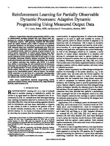
Supervised Learning focuses on learning a function given a set of input-output examples. A lot of models have been proposed mainly for continuous output tasks (i.e. regression) or classification tasks. A recent trend is to consider structured outputs such as sequences, trees or graphs. Structured Prediction (SP) is motivated by the amount of applications which are naturally described with such data. Such applications include prediction of protein structure in bio-informatics, image restoration, speech processing, handwriting recognition and several natural language processing tasks such as part-of-speech tagging, named entity extraction, sentence parsing or automatic translation. For example, in the handwriting recognition task, illustrated in figure 1, inputs are sequences of handwritten characters (e.g. gray-scale bitmaps) and outputs are sequences of labels identifying recognized characters. Most SP challenges come from the combinatorial nature of the prediction process i.e. the number of possible outputs is usually exponential with respect to the size of the input. Some new task-independent SP models have been proposed during the last years. These models have shown to perform well on simple SP tasks like sequence
Fig. 1. Two examples of Structured Prediction. Left: sequence labeling, the input X is a sequence of handwritten characters and the output Y is a sequence of labels identifying the recognized characters. Right: tree transformation, X is a an HTML tree from the web and Y is an XML tree with additional semantic information.
labeling but they often suffer from scaling problems on more complex tasks. In order to treat SP tasks with larger output spaces, a recent idea is to consider the prediction process as a sequential decision problem. For example, in handwriting recognition, one can build the correct output by taking one decision per character (recognize an ’s’, recognize an ’t’, ...). A more complex example is tree transformation, where decisions correspond to node creations, displacements or deletions. In order to construct the output structure, these decisions are performed sequentially. Decisions are interdependent, for example in figure 1 (left), the decision concerning partially hidden characters can be made easier thanks to previous easy character-recognition decisions. In this paper, we investigate the application of classical reinforcement learning algorithms to SP tasks. Therefore, we introduce a new framework called SPMDP which is a formulation of SP based on Markov Decision Processes. We show the equivalence between learning the optimal policy in SP-MDP and minimizing the empirical risk of the corresponding SP problem. Thanks to this equivalence, we can apply general reinforcement learning technics to SP problems. Our experiments focus on the two SP tasks illustrated in figure 1. Sequence labeling is probably the simplest and most studied SP task. Our experiments show the competitiveness of general RL algorithms against state-of-the-art SP models on this task. Tree transformation is a challenging SP task. The specific applications considered here imply trees containing more than one thousand nodes, very large description spaces (up to 106 dimensions) and an infinite state space. General RL algorithms show successful results on several real-world applications where previous SP methods failed. The paper is structured as follows. First, we introduce the field of SP and give an overview of existing methods in section 2. We then describe the SP-MDP formulation and show the equivalence between learning a policy in SP-MDP and solving the SP problem in section 3. We demonstrate the interest of the RL approach, with several experiments on sequence labeling and tree transformation tasks in section 4.
2
Structured Prediction
In this section, we define Structured Prediction and give an overview of existing SP methods. We focus on task-independant SP models: those which are not restricted to a particular data structure. 2.1
Formalism
The aim of SP is to learn a function which maps inputs x ∈ X to outputs y ∈ Yx , where the outputs are objects which have a structure, such as sequences, trees or graphs. X is the set of all possible inputs and Yx is the set of candidate outputs for a given input x. We denote by Y = ∪x∈X Yx the full output space. For learning, the user supplies a set of examples D = {(xi , yi )}i∈[1,n] . These examples are supposed to be independently and identically sampled from an unknown distribution DX ×Y . In order to evaluate the quality of a prediction, we ˆ instead use a loss function ∆(ˆ y, y∗ ) which quantifies how bad it is to predict y ∗ of y . The models introduced in the following are parameterized by a vector θ ∈ Rd and we denote fθ the prediction function corresponding to parameters θ. Two problems have to be solved in SP: • Inference. Given the parameters θ and an input x, the inference consists ˆ among all candidates Yx . In most SP problems, the in selecting an output y number of candidates is exponential in the size of the input. The predicted ˆ = fθ (x), should have a low loss value ∆(ˆ output, denoted y y, y∗ ). • Training. Given the set of examples D and the loss function ∆, training is the process of searching the best parameters θ that minimize a global loss over the training set. Formally, learning corresponds to minimizing the expected risk defined as follows: θ∗ = argmin Ex,y∼DX ×Y {∆(fθ (x), y)} θ∈Rd
Since the distribution DX ×Y is unknown, the expected risk cannot be computed and the methods usually try to minimize the empirical risk defined over the training set: X 1 θ∗ = argmin ∆(ˆ y = fθ (x), y∗ ) θ∈Rd N ∗ (x,y )∈D
2.2
Compatibility Based Models
One of the first ideas of SP was to generalize existing classification methods to structured outputs. Some new methods have been proposed which are based on a compatibility function F (x, y; θ) that measures how good is the output y given an input x. The classification function is thus defined as: fθ (x) = argmax F (x, y; θ) y∈Yx
A common choice is to choose F as a linear function: F (x, y; θ) =< θ, φ(x, y) > where < ., . > denotes the scalar product and φ is an input-output jointdescription function. Such a function jointly describes an input x and a corresponding candidate output y as a feature vector in Rd . Compatibility-based models differ in the meaning which is associated to the compatibility function and in the way to learn the θ parameters. The Structured Perceptron [1] is a generalization of the classical Perceptron which was first applied to natural language parsing. Learning is performed by simulating inference, and correcting the weight vector each time a wrong output is predicted. No special meaning is given to the compatibility function except the requirement that the correct output should have higher scores than wrong outputs. Conditional Random Fields (CRFs) [2] use a log-linear probability function to model the conditional probability of an output y given an input x. CRFs are graphical models where Markov assumptions are used in order to make inference tractable. This allows to express the probability of an output as a product over output sub-structures. Several methods extending the ideas of Support Vector Machines to SP have been proposed. SVM for Interdependent and Structured Output spaces (SVMISO, also known as SVMstruct ) [3] is a natural generalization of maximum margin classification to structured outputs. Maximum Margin Markov Network (M 3 N ) [4] is a generalization of probabilistic graphical models which is trained with a discriminant criterion. Both methods try to find parameters θ that lead to large margins: i.e. large score differences between correct and wrong outputs. They differ in the way constraints are defined and handled for the optimization. All compatibility-based models assume that inference can be solved efficiently. This optimization step which is involved in both learning and inference, has mostly been tackled with dynamic programming techniques. This has two major drawbacks. First, dynamic programming requires strong independence assumptions which are often unrealistic for real-world data. For example, in sequence labeling, it is often assumed that a label only interacts with the previous and next labels. Second, even with such independence assumptions, dynamic programming algorithms may have a prohibitive complexity. For example, when predicting trees, the best dynamic programming algorithms have a cubic complexity in the number of leaf nodes. This limits the use of such methods to small trees, e.g. less than 50 nodes. This family of methods is unable to deal with large-scale collections and complicated structured output and are limited to simple tasks like sequence labeling for example. 2.3
Incremental Models
Recently, a new idea has emerged from the field of SP. Instead of modeling a compatibility function and then solving a complex optimization problem, it is
possible to directly learn the prediction process. Instead of modeling what a good prediction looks like the Incremental models directly model how to build the good prediction. This simple idea thus suggests to integrate learning and searching into a sequential prediction process. This process starts with an empty initial partial output. Each decision correspond to an elementary modification of the output being predicted. States contain partial outputs and final states contain complete outputs. Incremental Parsing [5] is one of the first models using the idea of incremental prediction. This model was introduced in the context of natural language parsing, where inputs are sequences of words and outputs are parse trees. Incremental Parsing is built around a Perceptron which assigns ranking scores to partial outputs. The inference is performed greedily by making decisions that maximize the immediate ranking score. Learning is performed by repeating the following process: run the inference procedure until a wrong decision happens, stop inference and make an elementary correction of the Perceptron. Incremental prediction was popularized by LaSO [6] which is probably the first general Incremental SP model. LaSO relies on a beam-search procedure. The selection of partial outputs in the beam-search is computed by using a Perceptron. LaSO assumes that the whole path leading to the correct output is known for all examples. Learning repeats the following steps until convergence: run the inference procedure until the correct path leaves the beam, make an elementary correction of the Perceptron, re-insert the correct path in the beam and continue. Searn [7] is another general Incremental SP model developed later. In Searn, the decision maker is modelled by a classifier of any type (e.g. Support Vector Machines or Decision Trees). Searn assumes that for each learning example, we know an optimal decision maker. This decision maker knows the best decision to perform for all states of the prediction space. Searn uses an iterative batchlearning approach. At each Searn iteration, a mixture of the optimal decision maker and the learnt decision maker is used to perform inference on all learning examples. For each visited state, one classification example is created. At the end of the iteration, a new classifier is learnt on the basis of these new classification examples. This is repeated until convergence. Searn has shown to be efficient on numerous task and is considered as a general-purpose state-of-the-art SP model.
3
Structured Prediction with Markov Decision Processes
In this section, we introduce a new formulation of SP that is based on Markov Decision Processes. SP-MDPs are MDPs that model the inference process of a structured prediction. The main contribution of this paper is to show that learning the optimal policy in an SP-MDP is equivalent to solving the corresponding SP problem, i.e. minimizing the empirical risk. This original formulation allows to apply general-purpose Reinforcement Learning algorithms to SP tasks. In section 4, we show the competitiveness of such general algorithms against SP state-of-the-art methods. Contrary to LaSO and
Searn, our approach of SP does not rely on any additional assumption such as the availability of optimal trajectories or the availability of the optimal policy.
Fig. 2. Handwritten recognition SP-MDP. Circles are states and links are transitions. Each state contains the input and a partial output. Here, the input is a sequence of three black-and-white bitmaps representing handwritten digits. Partial outputs are partially recognized sequences of digits. The bottom double circled states are final states containing complete outputs.
3.1
SP Markov Decision Process
We adopt the formalism of deterministic MDPs (S, A, T , r) where S is the statespace, A is the set of possible actions, T : S × A → S is the transition function between states and r : S × A → R is the reward function. A SP-MDP is a deterministic MDP which models inference for a given SP task. SP-MDPs are illustrated in figure 2 and defined formally below: • States. Each state of a SP-MDP contains both an input x and a partial ¯ . Let Y¯ be the set of all possible partial outputs. The set of states of output y ¯ There is one initial state per possible input a SP-MDP is then S = X × Y. x: sinitial (x) = (x, �) where � is the initial empty solution. A set of examples D = {(xi , yi )}i∈[1,n] can thus be mapped to a set of corresponding SP-MDP initial states. Final states contain complete outputs which can be returned to the user. • Actions. Actions of SP-MDP concern elementary modifications of the partial ¯ . Those elementary modifications are specific to the SP problem. For output y example, in handwriting recognition, elementary modifications add a single label prediction to the current partial output. See section 4 for other examples of such ¯ ) be the set of modifications available given elementary modifications. Let M(x, y ¯ . The set As ⊂ A of actions available in the input x and the partial output y state s is defined as follows: ¯) As=(x,¯y) = M(x, y
• Transitions. SP-MDP transitions are deterministic and replace the current partial output by the transformed partial output. Transitions do not change the current input: ¯ ), a) = (x, a(¯ T ((x, y y)) where a(¯ y) denotes the modified partial output. • Rewards. In SP, the aim is to predict outputs which are as similar as possible to the correct outputs. Formally, we want to minimize the expectation of the SP loss function ∆. The reward function of an SP-MDP, which is discussed in next part, is closely related to ∆: ( −∆(a(¯ y), y∗ ), if a leads to a final state ¯ ), a) = r(s = (x, y 0, for all other states Note that the correct output y∗ is required to compute this reward function. 3.2
Learning a SP policy
In this part, we discuss the reward function of SP-MDPs and show that maximizing the expectation of perceived reward is equivalent to minimizing the empirical risk of SP. Remember that, in order to learn, we have access to a database of examples: inputs with their associated correct outputs. Since the computation of the reward requires the correct outputs, the rewards are only known for states that correspond to training examples. As illustrated by figure 3, we thus distinguish two parts of the state-space: the finite training subset and the remaining state-space.
Fig. 3. This figure illustrates a whole SP-MDP. The big circle denotes states that correspond to training SP examples: those where the reward function is known. For all states outside this circle, the reward function is unknown. More than a way to cope with the curse of dimensionality, we use function approximation in order to obtain policies able to generalize on the whole SP-MDP given only a small training subset.
The fact that the reward function is only known in a small subset of the statespace is the main particularity of SP-MDPs, when compared to usual sequential decision problems. The partial observability of the reward function leads us to the following observations. First, policy learning algorithms can only be applied to the training subset of the SP-MDP. Second, we are looking for policies with generalization capabilities. The knowledge acquired in the training subset should be applicable to the whole space, in order to make predictions on new inputs. In order to cope with large state-spaces and with the curse of dimensionality, RL algorithms using function approximation have been developed. We here focus on these algorithms for another reason: function approximation allows to learn the policy on a subset of the MDP and then to generalize on the whole MDP. Approximated RL algorithms learn parameterized policies πθ where θ ∈ Rd is the vector of parameters. The aim is to find a policy πθ∗ that maximizes the expectation of cumulative reward, given an initial state distribution D0 : πθ∗ = argmax Es0 ∼D0 {R(πθ , s0 )} θ
where the cumulative reward R(π, s0 ) is the sum of rewards perceived when PT following π starting from s0 : t=0 r(st , at ). We now show that finding the optimal policy in a SP-MDP is equivalent to minimizing the empirical risk (see part 2.1) of the SP problem. The key is that the cumulative reward of one episode in SP-MDP is the negative loss of the predicted output: R(πθ , s0 ) = r(s0 , a0 ) + · · · + r(sT −1 , aT −1 ) + r(sT , aT ) = 0 + · · · + 0 − ∆(a(¯ y), y∗ ) = −∆(¯ y = fθ (x), y∗ ) Let us consider the distribution D0D which uniformly picks examples from D to build initial states sinitial (x). When training a RL algorithm with the D0D initial states distribution, we are looking for the optimal policy: πθ∗ = argmax Esinitial (x)∼D0D {R(πθ , s0 )} θ∈Rd
= argmin Esinitial (x)∼D0D {∆(¯ y = fθ (x), y∗ )} θ∈Rd
= argmin θ∈Rd
1 N
X
∆(ˆ y = fθ (x), y∗ )
(x,y∗ )∈D
The optimal policy with the initial state distribution D0D is thus the policy which minimizes the empirical risk. This equivalence enables the use of general RL algorithms with function approximation like Sarsa, QLearning, Monte Carlo Control or TD(λ) [8]. 3.3
Representations
In order to use function approximation, we need an action-description function φ : S × A → Rd . This function describes state-action pairs with a set of d
feature-values. A feature can describe any joint aspect of the action and the current state. In the experiments described in section 4, we use large sparse feature spaces. Typically, the dimensionality d ranges from 103 to 106 . In order to build features, we use feature-templates and feature-generators. Consider for example the handwriting recognition task, where input characters are black-and-white bitmaps and actions concern single label predictions. In such a task, we want to have one feature per pixel and per label. We then introduce for example the following feature-template: ( 1, if (the pixel (x,y) is black) ∧ (the predicted label is l) fx,y,l (s, a) = 0, otherwise In order to describe a state-action pair, we use a feature-generator function which enumerates all the features that follow the feature-template and which are non-null. One example of such automatically generated feature is given below: ( 1, if (the pixel (3,7) is black) ∧ (a = ’S’) f3,7,0 S 0 (s, a) = 0, otherwise If we consider 10 × 10 black-and-white pixels and 26 possible labels, there are d = 2600 distinct features. However, for a given state-action pair, all the features corresponding to other labels than the selected one and those corresponding to white pixels are null. This leads to a sparse representation of less than 100 non-null features. In practice, sparsity allows for an efficient implementation where only the non-null features are taken into account. In our experiments, we use one to ten manually defined task-dependent feature-templates. This is enough to automatically generate up to millions of distinct features. Contrary to compatibility-based models which make decomposability assumptions on the description function (see part 2.2), the SP-MDP approach allows to include any long-term dependency in the description function. Sparse high-dimensional representations were introduced in the context of natural language processing [9] and have good practical properties: they are fast to compute and allow the use of simple, but powerful, linear learning machines.
4
Experiments
In this section, we describe several experiments performed with the SP-MDP approach on two SP tasks: sequence labeling and tree transformation. We introduce two main results in this section. Firstly, with the classical SP task of sequence labeling, we show the competitiveness of RL-based algorithms in comparison to state-of-art SP methods. Secondly, with the tree transformation task, we give a successful example of the capability of general RL algorithms to treat very large-scale SP tasks. Indeed, tree transformation deals with large trees (thousand nodes), complex transformations (structure and text processing, node creations, deletions and displacements) and very high dimensional learning (more than one
million dimensions). Up to our knowledge, SP-MDP is the only existing model able to handle this task yet. Traditional SP methods fail on this task, either due to their restrictive assumptions or due to their excessive complexity. 4.1
Sequence labeling
Sequence labeling amounts at predicting a label sequence y = (y1 , . . . , yT ) given an observation sequence x = (x1 , . . . , xT ). Each label yt corresponds to the observation xt and belongs to the set of possible labels L. Sequence labeling has various applications such as handwriting recognition, information extraction, named entity extractions or sentence chunking. We now detail the initial outputs, the actions and the loss function which define the sequence labeling SP-MDP. In order to represent partial outputs, we introduce a particular label ⊥ which denotes variables yt which have not been labeled yet. • Initial Outputs. The initial partial outputs in sequence labeling are sequences where no labels have been decided yet. An initial output � can thus be written � = (⊥, ⊥, . . . , ⊥). • Actions. Actions in sequence labeling correspond to single label prediction. We have compared two sets of actions: Left-to-right labeling and Order-free labeling. In the former, the first label y1 is decided at the first step, the second label y2 at the second step and so forth. At each step, there are card(L) possible actions which correspond to all possible labels for the current element. In order-free labeling, any unlabeled element can be labeled at any time (as in figure 2). This allows the system to first perform easy decisions (e.g. recognize easy letters) in order to gain more context for harder decisions (e.g. recognize a partially hidden letters). More details about this approach are provided in [10]. • Loss function. In order to evaluate the quality of a particular labeling, we use the Hamming Loss ∆. This loss function simply returns the number of wrong predicted elements: ∆(ˆ y, y∗ ) = card({i ∈ [1, T ], yˆi 6= yi∗ }). • Datasets. We performed our experiments on three classical sequence labeling datasets: – Spanish Named Entity Recognition (NER) This dataset, introduced in the CoNLL 2002 shared task1 , is made of spanish sentences where the aim is to find persons, locations and organisms names (there are 9 distinct labels in L). We used two train/test splits NER-large (8,324 training sentences) and NER-small (300 training sentences), as in [7] and [3]. Features include the words, the prefixes and suffixes of the words in a window of +/- 2 words. – Chunk This dataset put forward by [11] and introduced in the CoNLL2000 shared task2 is composed of sections of the Wall Street Journal corpus. The aim is to split sentences into non-overlapping nominal groups. There are 1 2
http://www.cnts.ua.ac.be/conll2002/ner/ http://www.cnts.ua.ac.be/conll2000/chunking/
three labels (BIO encoding): Begin of a new group, Inside a group, Outside a group. Input features include the words, prefixes, suffixes and part-of-speech of surrounding word. – HandWritten This corpus was created for handwritting recognition and was introduced by [12]. It includes 6,600 sequences of handwritten characters corresponding to 6,600 words collected from 150 subjects. Each word is composed of letters, which are 8 × 16 pixels images, rasterized into a binary representation. As in [7], we used two variants of the set: HandWritten-small (10% words for training) and HandWritten-large (90% words for training). Letters are described using one feature per pixel. Left To Right Sarsa RankingRL NER-small 91.90 93.67 NER-large 96.31 96.94 HandWritten-small 68.41 74.01 HandWritten-large 80.33 83.80 Chunk 96.08 96.22 NER-large ≈ 35min ≈ 25min HandWritten-large ≈ 15min ≈ 12min
Searn 93.8 96.3 64.1 73.5 95.0 ≈ 6h ≈ 3h
Order Free Sarsa RankingRL 91.28 93.35 96.32 96.75 70.63 73.57 79.59 84.08 96.17 96.54 ≈ 11h ≈ 8h ≈ 6h ≈ 4h
Non-incremental CRF SVMstruct 91.86 93.45 96.96 66.86 76.94 75.45 96.71 ≈ 8h > 3 days ≈ 2h > 3 days
Table 1. Top: percentage of correctly predicted labels on the testing set per dataset and model. Bottom: training times of each model with a traditional desktop machine. On some datasets, denoted by −, SVMstruct required too much memory to be applicable.
• Models. Experiments have been performed with the left-to-right and orderfree models combined with two algorithms: an approximated Sarsa(0) algorithm and the RankingRL algorithm proposed in [10]. Briefly, instead of learning an action-value which is the expectation of future discounted rewards, this algorithm learns to rank actions directly: only the order of the learnt action-scores matters. In all cases, we use �-greedy sampling, where � decreases exponentially with the number of learning iterations. The discount and learning rate parameters have been tuned manually. We compare the RL-based methods with two non-incremental state-of-the-art sequence labeling models: Conditional Random Fields3 and SVMstruct 4 (see part 2.2). We also compare with an existing Incremental SP method: Searn5 (see part 2.3). • Results. The results of our experiments are given in table 1. On all datasets, the RL based methods are competitive with state-of-the-art sequence labeling methods which demonstrates clearly the interest of our approach. order-free and left-to-right models give similar results on these experiments; see [10] for a discussion on these variants. Furthermore, for comparable performance, we have significantly lower training times than those of the non-Incremental models. It should also be noted, that inference in incremental model is several orders faster, 3 4 5
FlexCRFs implementation: http://flexcrfs.sourceforge.net. SVMstruct implementation: http://svmlight.joachims.org/svm struct.html Searn implementation: http://searn.hal3.name
since it simply consists in greedily executing the learnt policy (instead of solving a global optimization problem). These low training and inference times, allow us to consider much harder tasks than the simple sequence labeling, such as the tree transformation task described below. 4.2
Tree Transformation
We consider here a tree transformation task where both the inputs and outputs are ordered labeled trees. The applications we present deal with semi-structured textual documents. They consist in converting weakly structured (flat text or HTML) documents into highly structured XML documents. The main challenges of this tree transformation task come from the size of the documents, the complexity of the transformations and the huge number of training examples. In order to perform tree transformation, we represent the input trees as a sequence of in-context leaves: x = (x1 , . . . , xT ). Each leaf xi is a feature vector describing the leaf textual content and the context of the leaf (e.g. parent labels and sibling labels). • Initial Outputs. The initial outputs are composed of a single root node. • Actions. The key idea of our SP-MDP is that one leaf xt is processed per time step t. Processing a leaf means adding its textual content somewhere into the partial output tree. Either the textual content can be added into an existing node, or new nodes can be created to store the textual content. An action consists in two steps: first it selects an internal node of the partial output tree; then it creates new nodes from this location until a leaf where the textual content is added. This leads to a very large action space which is determined by a simple preprocessing of the examples dataset (see [13] and [14]). We furthermore consider a SKIP action which allows to ignore the current textual content. • Loss function. In order to evaluate the quality of an output, we used three tree-similarity functions. Fcontent measures the proportion of correctly labeled leaves. Fpath measures the proportion of correctly recovered paths. A path is a sequence of labels from the root node until a leaf node. Fstructure measures the proportion of correctly recovered subtrees. The latter is very strict and decreases quickly with only a few errors. For a single labeling error in a leaf, Fstructure typically equals to ≈ 80%. See [13] for more details. The loss function used in learning is the negative Fstructure score between the predicted and the correct output. • Datasets. We used four large-scale real-world datasets and one small dataset: – INEX IEEE [15]. The INEX IEEE corpus is composed of 12017 scientific articles in XML format, coming from 18 different journals. The documents are given in two versions: a flat segmented version and the XML version. The tree transformation task aims at recovering the XML structure using only the text segments as input. – Mixed Movies [15]. The second corpus is made of more than 13000 movie descriptions available in three versions: two mixed different XHTML versions
and one XML version. This corresponds to a scenario where two different websites have to be mapped onto a predefined mediated schema. The transformation includes node suppression and some node displacements. – Wikipedia [16] This corpus is composed of 12,000 wikipedia pages. For each page, we have one XML representation dedicated to wiki-text and the HTML code. The aim is to use the low-level information available in the HTML version, to predict an high-level representation. – RealEstate6 This corpus, proposed by Anhai Doan is made of 2,367 dataoriented XML documents. The documents are expressed in two different XML formats. The aim is to learn the transformation from the format to the other. – Shakespeare7 [17] This corpus is composed of 60 Shakespearean scenes. These scenes are small trees, with an average length of 85 leaf nodes and 20 internal nodes over 7 distinct tags. Dataset INEX IEEE Flat → XML Mixed Movies HTML → XML Wikipedia HTML → XML RealEstate XML→ XML Shakespeare Flat → XML
Size AvNodes NumLabels
Model
Fcontent Fpath Fstructure
12,017 ≈ 700
139
Sarsa
75.8 % 74.4 % 67.5 %
13,038 ≈ 100
40
Sarsa
79.2 % 77.8 % 64.5 %
12,000 ≈ 200 2,367 ≈ 34
256 37
Sarsa Sarsa PCFG+ME Sarsa PCFG+ME
60
≈ 105
7
80.2 99.9 99.9 94.4 98.7
% 74.3 % 65.6 % % 99.9 % 99.9 % % 7% 49.8 % % 93.2 % 87.5 % % 97% 94.7 %
Table 2. This table summarizes our experiments. From left to right: the dataset, dataset statistics (the number of documents, the average number of nodes in correct output documents and the number of distinct labels in output documents), the model and the three average similarity scores between predicted and correct outputs on the test set (Fcontent , Fpath and Fstructure ).
• Models. Each corpus is split into two parts: 50% for training and 50% for testing. Our model is the approximated-Sarsa(0) algorithm applied to the SPMDP described above. We only have one baseline on two datasets because most existing SP methods do not scale with our large datasets. The baseline itself does not scale on our three large datasets. The model PCFG+ME [17] can be seen as a compatibility based model for the tree transformation problem. It models the probability of outputs by using probabilistic context free grammars (PCFG) and maximum-entropy (ME) classifiers. Inference is then performed with a dynamicprogramming algorithm which has a cubic complexity in the number of input leaves. LaSO cannot be applied because we do not have access to correct paths for learning examples (see part 2.3). Searn cannot be applied because we do not have access to an optimal decision maker. Indeed, given a partial output tree and 6 7
http://www.cs.wisc.edu/ anhai/ http://metalab.unc.edu/bosak/xml/eg/shaks200.zip
the target output tree, the optimal decisions are those which minimize the treeedit distance between both trees. The best algorithms that compute tree-edit distances have at least a cubic complexity in the number of nodes. Due to the large size of our trees, these computations are not tractable so that we cannot compute the optimal decisions. • Results. The results of our experiments are given in table 2. All Fcontent scores are greater than 75 % while the more difficult Fstructure is still greater than ≈ 60 %. These scores are encouraging when considering the intrinsic difficulty of the tree transformation tasks. With INEX IEEE for example, the only hints for predicting one label among more than 100 labels come from the textual content of the input document (length, case, first and last words, ...). On the small datasets, the scores of Sarsa are slightly lower than those of the PCFG+ME baseline. This may due to the fact that PCFG+ME performs a global optimization using dynamic programming whereas Sarsa performs a greedy inference of the output tree. Greedy inference slightly degrades performance but it brings speed (most of document are inferred in less than one second) and scalability. Finally, an interesting result is that with a general reinforcement learning, we are able to solve a problem where previous SP methods failed.
5
Conclusion
In this paper, we introduced the structured prediction problem and gave an overview of some well-known methods for solving it. We introduced the SP-MDP formulation of structured prediction, which allows to apply general reinforcement learning algorithms to sequence, tree or graph prediction problems. Our experiments show that these general RL technics are often competitive against specialized SP algorithms. Furthermore, our approach requires less assumptions than the previous SP approaches, which allows us to deal with a complex and large scale tree transformation task. From the point of view of reinforcement learning, our problems are original on a number of aspects: the reward is only known for a subset of the space, the MDPs are discrete and very-large and we put a special emphasis on the generalization capabilities of the learnt policies. Given this unusual setting, we believe that the explicit bridge between SP and reinforcement learning may lead both domains to cross-fertilize and mutually reinforce each other.
References 1. Collins, M.: Discriminative training methods for hidden markov models: Theory and experiments with perceptron algorithms. In: EMNLP. (2002) 2. Lafferty, J., McCallum, A., Pereira, F.: Conditional random fields: Probabilistic models for segmenting and labeling sequence data. In: ICML’01. (2001) 3. Tsochantaridis, I., Hofmann, T., Joachims, T., Altun, Y.: Support vector machine learning for interdependent and structured output spaces. In: ICML’04. (2004) 4. Taskar, B., Guestrin, C., Koller, D.: Max-margin markov networks. In: NIPS. (2003)
5. Collins, M., Roark, B.: Incremental parsing with the perceptron algorithm. In: ACL’04, Barcelona, Spain (July 2004) 111–118 6. Daum´e III, H., Marcu, D.: Learning as search optimization: Approximate large margin methods for structured prediction. In: ICML, Bonn, Germany (2005) 7. Daum´e III, H., Langford, J., Marcu, D.: Search-based structured prediction. (2006) 8. Sutton, R., Barto, A.: Reinforcement learning: an introduction. MIT Press (1998) 9. Berger, A., Della Pietra, S., Della Pietra, V.: A maximum entropy approach to natural language processing. In: Computational Linguistics. (1996) 10. Maes, F., Denoyer, L., Gallinari, P.: Sequence labelling with reinforcement learning and ranking algorithms. In: ECML, Varsaw, Poland (2007) 11. Ramshaw, L., Marcus, M.: Text chunking using transformation-based learning. In Yarovsky, D., Church, K., eds.: Proceedings of the Third Workshop on Very Large Corpora, Somerset, New Jersey, ACL (1995) 82–94 12. Kassel, R.H.: A comparison of approaches to on-line handwritten character recognition. PhD thesis, Cambridge, MA, USA (1995) 13. Maes, F., Denoyer, L., Gallinari, P.: Xml structure mapping application to the pascal/inex 2006 xml document mining track. In: INEX, Dagstuhl, Germany (2007) 14. Maes, F., Denoyer, L., Gallinari, P.: Apprentissage de conversions de documents semi-structures a partir d’exemples. In: CORIA, Tregastel, France (2008) 15. Denoyer, L., Gallinari, P.: Report on the xml mining track at inex 2005 and inex 2006. SIGIR Forum (2007) 79–90 16. Denoyer, L., Gallinari, P.: The wikipedia xml corpus. SIGIR Forum (2006) 17. Chidlovskii, B., Fuselier, J.: A probabilistic learning method for xml annotation of documents. In: IJCAI. (2005)