Manipulating large-scale structures in a turbulent ...

Manipulating large-scale structures in a turbulent boundary layer using a wall-normal jet

by Murali Krishna Talluru

Submitted in total fulfilment of the requirements of the degree of Doctor of Philosophy

January 2014 Department of Mechanical Engineering UNIVERSITY OF MELBOURNE

Contents Abstract

iv

Declaration of Authorship

vi

Acknowledgements

vii

List of Figures

viii

List of Tables

xi

List of Abbreviations

xii

1 Introduction 1.1 Motivation . . . . . . . . . . . . . . . . . . . . . . . . . . . . . . . . 1.2 Thesis outline . . . . . . . . . . . . . . . . . . . . . . . . . . . . . .

1 2 6

2 Literature Review 2.1 Coherent structures . . . . . . . . . . . . . . . . . . . . . . . . . . 2.1.1 Near-wall structures, hairpin vortices, packets of hairpin vortices . . . . . . . . . . . . . . . . . . . . . . . . . . . . . . 2.1.2 Outer-layer structures . . . . . . . . . . . . . . . . . . . . 2.2 Large and very large-scale motions in the log-region . . . . . . . . 2.2.1 Influence on the near-wall structures . . . . . . . . . . . . 2.3 Turbulent skin-friction reduction techniques . . . . . . . . . . . . 2.3.1 Large eddy break up systems (LEBUs) . . . . . . . . . . . 2.3.2 Riblets . . . . . . . . . . . . . . . . . . . . . . . . . . . . . 2.3.3 Wall blowing and suction . . . . . . . . . . . . . . . . . . . 2.3.4 Spanwise wall oscillation . . . . . . . . . . . . . . . . . . . 2.3.5 Vortical flow . . . . . . . . . . . . . . . . . . . . . . . . . . 2.3.6 Active control . . . . . . . . . . . . . . . . . . . . . . . . . 2.4 Summary . . . . . . . . . . . . . . . . . . . . . . . . . . . . . . .

.

9 9

. . . . . . . . . . . .

11 18 19 23 27 28 30 32 33 34 36 39

i

Contents

ii

3 Experimental set-up 3.1 Facility . . . . . . . . . . . . . . . . . . . . . . . . . . . . . . . . . 3.1.1 Test section . . . . . . . . . . . . . . . . . . . . . . . . . . 3.1.2 Wall-normal Traverse . . . . . . . . . . . . . . . . . . . . . 3.2 Constant temperature anemometry . . . . . . . . . . . . . . . . . 3.2.1 Traversing hot-wire probe . . . . . . . . . . . . . . . . . . 3.2.2 Cross-wire probe . . . . . . . . . . . . . . . . . . . . . . . 3.2.3 Hot-film sensors . . . . . . . . . . . . . . . . . . . . . . . . 3.2.4 Single and two-point correlations: hot-wire and hot-film sensors . . . . . . . . . . . . . . . . . . . . . . . . . . . . . . 3.2.5 Filtering of hot-film signals . . . . . . . . . . . . . . . . . . 3.3 Measurement stations . . . . . . . . . . . . . . . . . . . . . . . . . 3.4 Wall-normal jet . . . . . . . . . . . . . . . . . . . . . . . . . . . . 3.4.1 Characteristics of jet . . . . . . . . . . . . . . . . . . . . . 3.4.2 Jet duty cycle . . . . . . . . . . . . . . . . . . . . . . . . . 3.4.3 Evolution of jet into the boundary layer . . . . . . . . . . 3.4.4 Spanwise movement of the jet . . . . . . . . . . . . . . . . 4 Skin-friction measurements using drag balance 4.1 Introduction . . . . . . . . . . . . . . . . . . . . 4.2 Drag balance . . . . . . . . . . . . . . . . . . . 4.3 Calibration . . . . . . . . . . . . . . . . . . . . 4.4 Frequency response of drag plate . . . . . . . . 4.5 Results and discussion . . . . . . . . . . . . . . 4.6 Summary and conclusions . . . . . . . . . . . .

. . . . . .

. . . . . .

. . . . . .

. . . . . .

. . . . . .

. . . . . .

. . . . . .

. . . . . .

. . . . . .

. . . . . .

. . . . . . .

41 41 44 45 48 48 50 53

. . . . . . . .

55 57 58 62 63 64 64 66

. . . . . .

69 70 72 75 77 78 82

5 Three-dimensional conditional view of large-scale structures in the log-region 5.1 Background . . . . . . . . . . . . . . . . . . . . . . . . . . . . . . . 5.2 Validation of sub-miniature cross-wire probe . . . . . . . . . . . . . 5.3 Three dimensional conditional view . . . . . . . . . . . . . . . . . . 5.3.1 Velocity fluctuations . . . . . . . . . . . . . . . . . . . . . . 5.3.2 Amplitude modulation of small-scale energy . . . . . . . . . 6 Evolution of large-scale structures 6.1 Convection velocity . . . . . . . . . . . . . . . . . . . . . . . . . . 6.2 Downstream development of correlation map of skin-friction fluctuations . . . . . . . . . . . . . . . . . . . . . . . . . . . . . . . . . 6.3 Conditional results . . . . . . . . . . . . . . . . . . . . . . . . . . 6.3.1 Mean Velocity . . . . . . . . . . . . . . . . . . . . . . . . . 6.3.2 Streamwise turbulence intensity . . . . . . . . . . . . . . . 6.4 Evolution of the conditional structure of large-scale events . . . . 6.5 Amplitude modulation of small-scale energy . . . . . . . . . . . . 7 Controlling large-scale structures (off-line)

84 85 86 90 91 95

101 . 102 . . . . . .

105 107 108 113 117 124 129

Contents 7.1 7.2 7.3 7.4

7.5

Convection velocity of the jet . . . . . . . . . . . . . . . . . . . Off-line control scheme . . . . . . . . . . . . . . . . . . . . . . . Conditional averages - definitions . . . . . . . . . . . . . . . . . 7.3.1 Mean velocity - modified boundary layer . . . . . . . . . Modification of the conditional structure of large-scale structures 7.4.1 Optimum time-delay . . . . . . . . . . . . . . . . . . . . 7.4.2 Orientation of Jet . . . . . . . . . . . . . . . . . . . . . . Threshold and length of detection events . . . . . . . . . . . . .

iii . . . . . . . .

8 Conclusions and Future work 8.1 Evolution of the conditional structure in a canonical flow . . . . . 8.2 Off-line control scheme . . . . . . . . . . . . . . . . . . . . . . . . 8.3 Future work . . . . . . . . . . . . . . . . . . . . . . . . . . . . . .

. . . . . . . .

131 133 136 138 144 146 154 163

168 . 169 . 170 . 171

Abstract Experiments are carried out in high Reynolds number turbulent boundary layers to explore the possibility of reducing the turbulence levels within the boundary layer. In particular, we here use active control in a novel attempt to control the large-scale structures that reside in the logarithmic and wake regions of a turbulent boundary layer. Besides, an unique drag balance facility has been built to obtain direct skinfriction measurements in a high Reynolds number turbulent boundary layer. The technique uses a large floating plate to calculate the overall skin-friction drag acting on it when there is a fluid flow over it. Initial measurements using this facility closely agreed to the existing empirical relations on skin-friction, suggesting that it could be used reliably in future to implement various drag reduction studies. At first, the large-scale structures are detected and quantified across the entire boundary layer. The foot-print of the large-scale structures at the wall is used to detect their passage. Based on such detection, it has been possible to extract the conditional three-dimensional view of the large-scale structures. These structures are found to be very long of the order of 6δ and inclined at a characteristic angle of 120 in the streamwise direction. A large-scale, low-speed region is flanked on either side by regions of high-momentum of similar general form. The associated spanwise and wall-normal velocity fluctuations revealed the presence of large-scale roll modes. The phenomenon of amplitude modulation of the small-scales by the large-scale motions is universally observed in all the velocity components and the Reynolds shear stress. The evolution of the large-scale structures has been studied by systematically increasing the separation distance between the reference wall shear-stress sensor and a measurement array. It is noticed that the large-scale structures correlate well with the skin-friction fluctuations for a very large streamwise distance (∼ 6δ). An interesting common behaviour is noticed in the conditional mean and turbulence intensity profiles beyond z/δ = 0.15. Above this location, the large-scale structures are seen to be convecting over a distance of 6δ with a negligible change in the correlation values with the skin-friction fluctuations at the wall. Finally, a rectangular wall-normal jet has been developed to perturb the largescale structures in the flow and an off-line control is simulated. Of the two jet

v orientations (streamwise and spanwise) tested, the streamwise aligned jet is found to modify the large-scale structures for greater streamwise distances. Based on several off-line control schemes, we found that the ideal scheme is that where the jet has been actuated for the entire length of the large-scale events. Furthermore, it has been observed that the control effect is maximum when the strength of the jet is correctly matched to the strength of the detected large-scale events. Overall, this study demonstrates the potential of using a wall-normal jet to modify the large-scale structures taking into account the geometry of the jet and the momentum input in relation to the boundary layer thickness and the momentum within the boundary layer. As a closing note, these results suggest that there is a better scope of targeting the large-scale structures and obtain skin-friction reduction by using multiple actuators and with a control scheme implemented in real-time.

Declaration of Authorship This is to certify that:



the thesis comprises only my original work towards the PhD except where indicated in the Preface,



due acknowledgement has been made in the text to all other material used,



the thesis is fewer than 100 000 words in length, exclusive of tables, maps, bibliographies and appendices OR the thesis is [number of words] as approved by the Research Higher Degrees Committee.

Signed:

Date:

vi

Acknowledgements Foremost, I would like to express my sincere gratitude to my advisers Prof Ivan Marusic and Assoc. Prof Nicholas Hutchins for their continuous support during my PhD study, for their patience, motivation, enthusiasm and immense knowledge. Their guidance helped me immensely through the entire course of my research and thesis-writing. I would like to thank the rest of my thesis committee: Dr Chris Manzie, Dr Jason Monty, Dr Daniel Chung, and Prof Min Chong for their encouragement, insightful comments, and questions which put me on the right course. I also thank Dr Saurabh Garg, Dr Kapil Chauhan and Dr Jimmy Phillip for sharing their research experiences and for their helpful suggestions throughout my PhD. My sincere thanks goes to my fellow friends in the Fluids Group: Brett Bishop, Dr Henry Ng, Dr Vigneshwaran K, Rio Baidya, Bagus Nugroho, Reza Medad, Charitha de Silva, Will Lee, and Tony Kwon for their unique friendship and support during difficult times. I also thank my very dear friends Ravikanth and Geethika who have become more like a family to me now. Thanks must also go to technicians Geoff Duke, Derek Jacquest and Mark Franzke for their assistance in building parts for my experiments. A special thanks goes to Emma Mitchell for her ever cheerful encouragement and help in dealing with all the administrative tasks of the University. I also thank my wife, Himabindu Devi, for her love and affection towards me especially during the final stages of my PhD. To my parents for their patience and encouragement in every step that I took in my student life. Finally, I express my deepest gratitude to my teacher at IIT Delhi who not only developed in me an interest in Fluid mechanics but also took great care to help students develop finer qualities in life, and thereby contribute positively to oneself and to the society at large.

vii

List of Figures 1.1

The organisation and dynamics of large-scale structures . . . . . . .

2.1 2.2 2.3

2.5 2.6 2.7 2.8

Stretched and lifted vortex element - Offen & Kline [1975] . . . . Counter-rotating vortex model of Blackwelder & Eckelmann [1979] Multiple hairpins stacking together from Head & Bandyopadhyay [1981] . . . . . . . . . . . . . . . . . . . . . . . . . . . . . . . . . Re dependence of entraining motions from Head & Bandyopadhyay [1981] . . . . . . . . . . . . . . . . . . . . . . . . . . . . . . . . . Nested packets of hairpin growing up from the wall . . . . . . . . Large-scale structures in a turbulent boundary layer . . . . . . . . Large-scale structures in a pipe flow . . . . . . . . . . . . . . . . . Conditional structure of large-scale events in a TBL . . . . . . . .

3.1 3.2 3.3 3.4 3.5 3.6 3.7 3.8 3.9 3.10 3.11 3.12 3.13 3.14 3.15 3.16 3.17

Three dimensional sketch of the Wind Tunnel Facility . . . . . . All sensors and actuators . . . . . . . . . . . . . . . . . . . . . . Two axis traverse assembly . . . . . . . . . . . . . . . . . . . . . Schematic drawing of the experimental set-up . . . . . . . . . . Specifications of hot-wire . . . . . . . . . . . . . . . . . . . . . . Schematic drawing of crosswire probe . . . . . . . . . . . . . . . Specifications of spanwise array of skin-friction sensors. . . . . Spanwise correlation of skin-friction sensors . . . . . . . . . . . Comparison of auto-correlation curves of hot-wire and a hot-film Gaussian filtering of hot-film . . . . . . . . . . . . . . . . . . . . Schematic drawing of the measurement stations . . . . . . . . . Variation of boundary layer thickness . . . . . . . . . . . . . . . Wall-normal jet . . . . . . . . . . . . . . . . . . . . . . . . . . . Specifications of duty cycle of the Jet . . . . . . . . . . . . . . . Mean velocity profiles - continuous jet . . . . . . . . . . . . . . Spanwise movement of the jet . . . . . . . . . . . . . . . . . . . Two orientations of the jet . . . . . . . . . . . . . . . . . . . . .

4.1

Three dimensional CAD model of drag balance, vidual components. . . . . . . . . . . . . . . . . Exploded view of Air-bearing assembly . . . . . Exploded view of Spanwise lock assembly . . . . Set-up of the load cell calibration . . . . . . . .

2.4

4.2 4.3 4.4

viii

with . . . . . . . . . . . .

all the . . . . . . . . . . . . . . . .

6

. 13 . 14 . 16 . . . . .

16 18 21 22 23

. . . . . . . . . . . . . . . . .

. . . . . . . . . . . . . . . . .

43 45 46 49 50 51 53 56 57 58 60 62 63 65 65 67 68

indi. . . . . . . . . . . .

. . . .

73 73 74 76

List of Figures

ix

4.5 4.6

Measured force value on the load cell against applied force . . . . Natural frequency of drag balance. The harmonics are also shown in the figure. . . . . . . . . . . . . . . . . . . . . . . . . . . . . . . 4.7 Comparison of Cf obtained using K´arm´an-Schoenherr fit and linear fit, in Reθ range obtained over the length of drag plate at the free stream velocity of U∞ = 20 m/s . . . . . . . . . . . . . . . . . . . 4.8 Typical unfiltered force signal from the transducer over a period of 100 seconds for U∞ ≃ 24 m/s . . . . . . . . . . . . . . . . . . . . 4.9 Comparison of Uτ with U∞ from the drag-balance with Clauser chart results of Hutchins et al. [2009] . . . . . . . . . . . . . . . . 4.10 Comparison of Cf values with established empirical relations for Cf with Reθ [Nagib et al., 2007] . . . . . . . . . . . . . . . . . . . . . . . . . . . . . .

. . . . . . . . .

. . . . . . . . .

. . . . . . . . .

. 76 . 78

. 79 . 80 . 81 . 82

5.1 5.2 5.3 5.4 5.5 5.6 5.7 5.8 5.9

Validation of u statistics - cross-wire probe . . . . . . . . . Validation of statistics of v, w, and −uw - cross-wire probe Iso-contours of u+ . . . . . . . . . . . . . . . . . . . . . . . Iso-contours of v + . . . . . . . . . . . . . . . . . . . . . . . Iso-contours of w + . . . . . . . . . . . . . . . . . . . . . . Roll-modes observed in the planes ∆x/δ = 0, 1 and 2. . . . Process of isolating small-scales . . . . . . . . . . . . . . . Iso-contours of small-scale variance of u, v, and w . . . . . Iso-contours of Reynolds shear stress . . . . . . . . . . . .

. . . . . . . . .

88 89 92 93 94 95 96 98 99

6.1 6.2 6.3 6.4 6.5 6.6 6.7 6.8 6.9 6.10 6.11 6.12 6.13 6.14 6.15 6.16

Determining Uc for unmodified flow . . . . . . . . . . . . . . . . . . 103 Two-dimensional correlation map . . . . . . . . . . . . . . . . . . . 106 Mean velocity profiles at different stations . . . . . . . . . . . . . . 110 Difference between the conditional and unconditional velocity profiles112 Schematic of a large-scale structure and a turbulent bulge . . . . . 112 Turbulence intensity profiles at different stations . . . . . . . . . . . 114 Difference between the conditional and unconditional variances . . . 116 Three-dimensional conditional structure - all stations . . . . . . . . 118 Spanwise–wall-normal view at ∆x/δ = 0 . . . . . . . . . . . . . . . 120 Variation of u+ |max with streamwise separation distance . . . . . . . 121 Spanwise–wall-normal planes at different stations . . . . . . . . . . 122 Difference . . . . . . . . . . . . . . . . . . . . . . . . . . . . . . . . 123 Contour lines at stations s0 to s7 . . . . . . . . . . . . . . . . . . . 124 Three-dimensional conditional structure of small-scales - all stations 126 Conditional small-scale variances . . . . . . . . . . . . . . . . . . . 128 Cartoon of the conditional structure of small-scale variance . . . . . 128

7.1 7.2 7.3 7.4 7.5

Detect and Fire . . . . . . . . . . . . . . . . . . . . . . . . . . . . . Comparison of the hot-wire and control signals of the jet . . . . . . Determining Uc of the jet . . . . . . . . . . . . . . . . . . . . . . . . Comparison of convection velocities of jet and large-scale structures Simulated control scheme . . . . . . . . . . . . . . . . . . . . . . . .

130 131 132 133 135

List of Figures 7.6 7.7 7.8 7.9 7.10 7.11 7.12 7.13 7.14 7.15 7.15 7.15 7.16

x 139 141 143 145 147 150 151 152 153 156 157 158

7.17 7.18 7.19 7.20 7.21

Comparison of mean velocity during continuous blowing . . . . . . Comparison of conditional mean velocity profiles at s3. . . . . . . . Effect of jet on U|h and U|l . . . . . . . . . . . . . . . . . . . . . . Change in the BL properties across the spanwise direction . . . . . Optimisation of delay for firing the jet. . . . . . . . . . . . . . . . . Canonical flow . . . . . . . . . . . . . . . . . . . . . . . . . . . . . . Modified flow - delay of T + = 594 . . . . . . . . . . . . . . . . . . . Modified flow - delay of T + = 108 . . . . . . . . . . . . . . . . . . . Comparison of results with different time-delays . . . . . . . . . . . Canonical and manipulated conditional averages . . . . . . . . . . . Caption over page . . . . . . . . . . . . . . . . . . . . . . . . . . . . Comparison between the streamwise and spanwise jet configurations Comparison of the streamwise and spanwise orientations of jet with the unmodified flow . . . . . . . . . . . . . . . . . . . . . . . . . . . Modified flow - streamwise jet . . . . . . . . . . . . . . . . . . . . . Modified flow- spanwise jet . . . . . . . . . . . . . . . . . . . . . . . Attempted control schemes . . . . . . . . . . . . . . . . . . . . . . . Attempted control schemes . . . . . . . . . . . . . . . . . . . . . . . Attempted control schemes . . . . . . . . . . . . . . . . . . . . . . .

8.1 8.2 8.3 8.4

Comparison of conditional mean velocity profiles at s3. . . . . . . Schematic of interaction between the bulges and the near . . . . Future control schemes . . . . . . . . . . . . . . . . . . . . . . . . Future control scheme involving multiple detections and actuators

172 173 174 175

. . . .

160 161 162 163 166 166

List of Tables 3.1 3.2 3.3

Normalised dimensions of sensor lengths of the cross-wire probe. . . 52 Dimensions and positions of all the sensors . . . . . . . . . . . . . . 54 Summary of Experiments - canonical boundary layer . . . . . . . . 61

4.1

Comparison of Uτ data with Hutchins et al. [2009] . . . . . . . . . . 81

5.1

Summary of mean properties - uvw . . . . . . . . . . . . . . . . . . 87

6.1 6.2

Convection velocity table. . . . . . . . . . . . . . . . . . . . . . . . 104 Table of symbols for different measurement stations. . . . . . . . . . 108

7.1 7.2 7.3

Convection velocity table with jet on. . . . . . . . . . . . . . . . . . 134 Comparison of time-delay . . . . . . . . . . . . . . . . . . . . . . . 148 List of threshold values and length of the detection events . . . . . 164

xi

List of Abbreviations TBL

Turbulent Boundary layer

ZPG

Zero Pressure Gradient

BLT

Boundary Layer Thickness

CTA

Constant Temperature Anemometry

NPL

National Physics Laboratory, UK

HWA

Hot Wire Anemometry

OHR

Over Heat Ratio

DNS

Direct Numerical Simulation

PIV

Particle Image Velocimetry

LES

Large Eddy Simulation

VLSM

Very Large Scale Motions

VITA

Variable Interval Time Averaging

IOI

Inner Outer Interaction model

LEBU

Large Eddy Break Up systems

OLM

Outer Layer Manipulators

HRNBLWT High Reynolds Number Boundary Layer Wind Tunnel MUCTA

Melbourne Uuniversity Constant Temperature Anemometer

xii

Nomenclature +

Viscous scaled parameters

∆τ

Time-shift between the hot-film and hot-wire signals

∆t

Time-shift at maximum correlation

∆xD Distance between the upstream and downstream sensor arrays ∆y

Spanwise separation between the reference hot-film and hot-wire sensors

δ

Boundary layer thickness

δ∗

Displacement thickness

uˆ

Total velocity signal

µs

The coefficient of static friction

ν

Kinematic viscosity of the fluid

Γ

Integrated value of Γ across the measurement locations

u2s

Time-averaged small-scale variance

φ

Angular displacement of the string

ρ

Density of the fluid

τw

Shear stress at the wall

θ

Momentum thickness

u˜2s |h Small-scale variance conditioned on high skin-friction event xiii

u˜2s |l

Small-scale variance conditioned on low skin-friction event

Cf

Coefficient of skin-friction

d

Hot-wire diameter

l

Etched length of hot-wire

Reδ∗

Reynolds number based on displacement thickness

Reτ

Friction Reynolds number or Karman number

Reθ

Reynolds number based on momentum thickness

ReDh Reynolds number based on hydraulic diameter Rex

Reynolds number defined based on streamwise development length

T

Total length of velocity signal

t

Sampling interval

T+

Non-dimensional time-delay

U

Mean velocity

u

Fluctuating velocity

u

Streamwise velocity fluctuations

u |hj

Velocity fluctuations conditioned on uτ ≥ 0 and j == 1

u |h

Velocity fluctuations conditioned on high skin-friction event

u |j

Velocity fluctuations conditioned on j == 1

u |lj

Velocity fluctuations conditioned on uτ < 0 and j == 1

u |l

Velocity fluctuations conditioned on low skin-friction event

u2

Time-averaged streamwise variance

U∞

Free stream velocity

Uτ

Mean friction velocity

uτ

Fluctuations in friction velocity

Uc

Convection velocity of large-scale structures

up

Predicted fluctuating velocity

v

Spanwise velocity fluctuations

Vr

Ratio of jet velocity and the free-stream velocity

w

Wall-normal velocity fluctuations

x

Streamwise axis

y

Spanwise axis

z

Wall-normal axis

Γ

Integrated sum of conditional fluctuations over a volume

u˜2 |h Mean variance conditioned on uτ > 0 u˜2 |l

Mean variance conditioned on uτ < 0

fs

Sampling frequency

h

Misalignment height

hfd

Downstream skin-friction sensor array

hfu

Upstream skin-friction sensor array

Chapter 1 Introduction An experimental facility has been developed with the intention of studying the connection between large-scale coherent structures and the near-wall skin-friction sensed at the wall. The aim is to implement effective perturbations to a canonical boundary layer with the goal of reducing the skin-friction drag. The underlying motivation is to make a detailed study of the large-scale structures, their growth in streamwise direction and their interaction with the near wall turbulence levels. In particular, we focus on modifying these long streamwise streaks that exist in a high Reynolds number turbulent boundary layer using a perturbation generated by a wall-normal rectangular jet. Through such methods we seek to understand the active dynamics between the large-scale coherent structures and the wall shearstress fluctuations, and thereby develop improved and practically feasible drag reduction techniques. We begin by characterising the large-scale structures in high Reynolds number turbulent boundary layers using conditional analysis which has been shown previously in the literature to faithfully represent the spatial characteristics of these structures. For the first time, detailed measurements are carried out at several locations in the streamwise direction, enabling the evolution of the large-scale conditionally averaged events to be studied. This has provided unique insights into the length and time-scales of the large-scale structures and how they influence the skin-friction fluctuations at the wall. An accompanying study is carried out to 1

Introduction

2

understand the conditional structure of the spanwise and wall-normal velocity fluctuations. This study reveals the three-dimensional nature of the large-scale events. Having obtained the three-dimensional organisation of large-scale structures, their streamwise evolution, and the modulating effect on the near wall structures, the characteristics are compared with those of a perturbed boundary layer. For this purpose, a wall-normal jet is constructed specifically for this study to modify the large-scales in the flow. As a first step, a simple off-line control scheme is developed and studied to understand the interactions between a wall-normal jet and a turbulent boundary layer. The effect of such a scheme is evaluated in a systematic manner from measurements at several downstream locations using hot-wire anemometry.

1.1

Motivation

Research on wall turbulence has been carried out for over 100 years and this is justified given its importance to a vast number of applications, which range from micro-scale biological sciences to large-scale atmospheric studies. Wall-turbulence is found in a wide range of engineering applications and remains one of the unsolved problems of classical physics. The focus of this research is the drag caused by turbulent boundary layers; the thin regions of turbulent flow close to a solid surface (for example, e.g., flow over aircraft, submarines, flow inside engines, and flow in chemical processing plants). A breakthrough in the control of wall-turbulence would be a substantial technological advancement with numerous benefits to society. Significant energy savings would be possible with skin-friction drag reduction, given its large contribution to total drag. This would decrease the pollutants and greenhouse gases in the atmosphere due to lower consumption of fuels. In general, fundamental understanding of turbulent flows is limited, mainly due to the non-linear interactions between different scales of motion that coexist within a turbulent boundary layer. Recent advances in the understanding of turbulent boundary layers has enabled the development of novel techniques in skin friction

Introduction

3

drag reduction. This research, from the early 1960s, led to the discovery that the turbulent boundary layer can at times exhibit high degrees of organisation in contrary to its then popular image. Far from being random, turbulent boundary layers possess recurrent features and flow topologies, collectively referred to as coherent structures. Following this discovery came the confirmation that these structures are substantial contributors to Reynolds stress and turbulence production in the boundary layer. This has opened up the prospects of controlling wall turbulence, a phenomena that has been long viewed as uncontrollable. Many attempts have been made to investigate the coherent structures and study the possibilities of controlling them. These can be broadly categorised into two strands. They are (i) prevention of vortex regeneration and (ii) large-scale flowmanipulation. The first involves strategies that aim to prevent vortex regeneration at the wall or that attempt to counteract the active dynamics of near-wall coherent structures, which scale with the viscous length [Gad el Hak, 1996]. Such methods involved the use of an extensive network of sensors and actuators in a closed loop control. However, such strategies are difficult to implement at practical Reynolds numbers. (For wall bounded flows, the relevant Reynolds number is Reτ = δUτ /nu, which is the non-dimensional parameter quantifying the ratio of inertial to viscous forces acting in the flow.) Here ν is the kinematic viscosity of the fluid, Uτ is the friction velocity and δ is the boundary layer thickness. For example, a normal cruising aircraft typically experiences a flow whose viscous length defined as ν/Uτ is O(1 micron). This requires a sensor whose dimension is of the order of 50ν/Uτ and hence a 1m2 area of the aircraft surface requires close to 108 sensor-actuator pairs. The second approach employs large-scale forcing and successful examples, at least in concept, include spanwise oscillation [Choi, 1989] and forcing the flow using large-scale streamwise vortices [Schoppa & Hussain, 1998]. In the latter case, drag reduction of 50% was reported in numerical simulations using the concept of spanwise-directed colliding jets in a low Reynolds number turbulent channel flow (Reτ = 180). A vast majority of previous works has tended to concentrate on those structures in the near-wall region for several reasons. At low Reynolds number typical of

Introduction

4

laboratory investigations, they are the most dominant contributors to turbulence production, accounting for a large peak in turbulence intensity near the wall. These observations made the near wall structures an obvious target and hence, most turbulent control techniques are developed to affect them. However, the scope of the utility of such techniques is quite limited as the smallest scales in the flow become even smaller at higher Reynolds number flows and hence such control schemes become increasingly difficult and impractical to implement at high Reynolds number. Recent studies, e.g., Adrian et al. [2000], ?, highlighted why the large-scale flow manipulations may be possible. Their studies were conducted at high Reynolds number flows and the results showed the presence of very large-scale motions (VLSMs, also referred to as ‘superstructures’) in the logarithmic region of a turbulent boundary layer. Although the understanding of these features is preliminary, they can at present be categorised as highly elongated regions of positive or negative velocity fluctuations extending over streamwise lengths of 15δ to 20δ. These structures have been observed universally in high-Re pipe, channel and flat plate boundary layers as well as in atmospheric surface layer studies. Besides the conspicuous presence of large-scale structures in high Reynolds number flows, these structures seem to be influencing the near wall turbulence levels. In separate DNS studies, Abe et al. [2004] noted a footprint from the outer-layer structure onto the near-wall region, observing that these large-scale structures contribute to the shear stress fluctuations. Tsubokura [2005] and Schlatter et al. [2009], respectively noted similar phenomenon from LES studies of pipe and channel flows and from DNS studies of flat plate boundary layer flow. The foot-print of these large-scale structures has been used by Hutchins et al. [2011] to study the three dimensional conditional structure of large-scale structures. They reported that these structures are forward leaning, flanked on either side by regions of opposite sign fluctuations in the spanwise direction, and in the mean sense, accompanied by large-scale counter rotating roll modes, see Dennis & Nickels [2011] and Hutchins et al. [2012].

Introduction

5

Furthermore, Hutchins & Marusic [2007b] inferred that the large outer-region motions extend down to the wall, and modulate the flow in the inner layer, including the buffer layer. Such interaction was also shown previously by Brown & Thomas [1977] and Bandyopadhyay & Hussain [1984]. Recently, this interaction was quantified by Mathis et al. [2009a], and formed the basis of a successful algebraic model by Marusic et al. [2010], wherein the statistics of the streamwise fluctuating velocity in the near-wall region could be predicted given only the large-scale velocity signature in the outer logarithmic region of a certain specific flow. This is followed by a conditional average study of small-scale turbulence by Hutchins et al. [2011], which observed that a high-speed structure is associated with the high skin-friction event and consisted of intense small-scale activity near the wall, switching to weaker small-scale fluctuations in the logarithmic region in a turbulent boundary layer. The discussion so far, is summarised in figure 1.1. The large-scale low-speed/highspeed structures are shown in blue/red colours, residing in the log-layer of a turbulent boundary layer. They extend over 15-20 δ streamwise distances and have associated roll-mode like structures, represented by circular arrows. The phenomenon of amplitude modulation is shown in the inset. Based on the strength of these findings, we raise the question,“Is it viable to specifically target the large-scale structures in order to control turbulence?” An attempt is made here to understand the physics of the flow, when a large-scale structure is perturbed. The approach is based on the current understanding of the organisation of large-scale structures. It is clear from the figure 1.1, that below a large-scale high speed structure (shown as the red region), there is increased turbulence activity near the wall and an associated increase in skin-friction. Hence, a high speed structure would seem to be an obvious target of any control strategy. Furthermore, there seems to be downward motions occurring in the flow during the passage of a high speed structure. A wall-normal jet is used to target the downward motions, and thereby weaken the bigger roll-mode like structures. The modification of the streamwise velocity fluctuations is used as a means of gauging the efficiency of our simulated control scheme.

Introduction

1.2

6

Thesis outline

Chapter 2 provides a literature survey of the previous studies related coherent structures, their interactions with the near wall turbulent structures and the current turbulent skin-friction reduction strategies. This chapter forms the basis for the hypothesis proposed in this study in perturbing the large-scale structures that exist in high Reynolds number flows. Substantial discussion is carried out on the importance of large-scale structures, their interaction with near-wall turbulence and the possibility of manipulating them as a means to reduce skin-friction at the wall. Chapter 3 documents the experimental set-up, and includes wind tunnel, instrumentation and calibration procedures used throughout the experiments. In a study of this nature, it is important to use a combination of sensors and actuators; some are used as detectors, while others are used to characterise the effects of a perturbation. The details of the hot-film sensor arrays, hot-wire and cross-wire probes and finally the jet are outlined. The specific advantage of the design of the measurement array becomes obvious from the fact that several measurements are

. Figure 1.1: The organisation and dynamics of large-scale structures in a turbulent boundary layer. From Marusic et al. [2010]

.

Introduction

7

needed in this work. Such a measurement array is required to study the streamwise evolution of the large-scale structures in a systematic manner. Also, some of the quantities and conditional averages used throughout the thesis are defined here to save space and avoid repetition of the analysis in later chapters. A stand alone work related to the development and validation of a large drag balance facility at the university of Melbourne has been documented in chapter 4 of this report. The uniqueness of the facility and the initial measurements from it are discussed in comparison to the existing empirical relations for skin-friction coefficient and also the previous measurements of skin-friction in the same wind tunnel facility. The measurements revealed the potential use of drag balance in conducting drag reduction techniques as a future study to the current one. In recent years, progress has been made in characterising the shape and organisation of large-scale structures, see Hutchins et al. [2011]. However, such a view is primarily limited to the streamwise velocity fluctuations and it is important to understand how other velocity fluctuations are correlated with the large-scale features in the flow. To this end, a direct extension of the work of Hutchins et al. [2011] is presented in chapter 5. Results based on conditional analysis of three velocity components are discussed, highlighting some of the key aspects of the three dimensional organisation of large-scale structures. The phenomenon of amplitude modulation is studied using the spanwise and wall-normal velocity components. An inference is also made that the current model of Marusic et al. [2010] in predicting streamwise fluctuations could be extended to cover other velocity fluctuations. The results from this chapter also provide some characteristic inputs to the control scheme discussed in chapter 7, such as the magnitude and penetration depth of the perturbation. A natural extension to chapter 5 is the study of the evolution of the conditional structure of large-scale structures in the streamwise direction. In chapter 6, several conditional results are presented from the measurements taken at different streamwise locations. The measurement array described in chapter 3 is particularly relevant to the measurements and analysis presented in this chapter.

Introduction

8

The results are used to understand the physics of the interactions between the large- and small-scale structures in the flow. Furthermore, the results also form a baseline case to compare the results obtained from the off-line simulated control scheme, presented in chapter 7. As a first step towards embarking on the control schemes aimed at modifying the large-scale structures in the flow, an off-line simulated control scheme is implemented in chapter 7. Experiments are carried out by periodically actuating the jet and simultaneously sampling all the sensors. In the post-processing stage, a simple control termed as ‘detect and fire’ is applied as a precursor to a real-time active control. Direct comparisons are made with a base-line study described in chapter 6 and conclusions are drawn on the effectiveness of the control scheme. The thesis concludes with Chapter 8, which summarises some of the key findings from the previous chapters. Recognising this study is only the beginning of flowcontrol strategies aimed at the large-scale structures in wall-bounded flows, it is very difficult to put a stop to this kind of study. Keeping these facts in mind, some suggestions are presented that could be carried out as possible future research work.

Chapter 2 Literature Review The literature review comprises of three sections: • § 2.1 Coherent structures • § 2.2 Very large-scale structures • § 2.3 Turbulent skin-friction reduction techniques Further studies relating to hot-wire anemometry and convection velocity of coherent structures in a turbulent boundary layer are discussed in the relevant sections of the thesis. This survey is primarily aimed at introducing the reader to the subject matter on which this study has been built. It presents a overview of the developments that have taken place to date, both in the fundamental understanding of the structure of a turbulent boundary layer and the evolution of flow control techniques.

2.1

Coherent structures

In a turbulent boundary layer, kinetic energy from the potential flow is dynamically converted into turbulent fluctuations and then dissipated by viscous forces. This process continues, such that the turbulent boundary layer is self-sustaining. 9

Literature Review

10

Researchers have sought, for as long as the above fact has been known, to understand how the turbulence in a boundary-layer is generated at the expense of the mean momentum, and how it is dissipated. This has been the motivation behind studying the structure of turbulence. The progress made, however, does not truly indicate the immense efforts that have been spent, reflecting the fundamentally complex nature of the turbulence phenomena. Over the last several decades, there has been an emergent acceptance that wallbounded turbulence is composed of a class of recurrent and quantifiable structures, collectively termed as ‘coherent structures’. These structures are shown to play an important role in turbulence production, being major contributors to the timeaveraged turbulence statistics including skin friction, as reviewed by Panton [2001]. For the purposes of this review, we will follow the definition of coherence, given by Robinson [1991].

..a three dimensional region of the flow over which at least one fundamental flow variable (velocity component, density, temperature etc.) exhibits significant correlation with itself or with another variable over a range of space and/or time that is significantly larger than the smallest scales of the flow.

This definition suits particularly well for the current study as it encapsulates the meaning of coherence in a turbulent boundary layer, without specifically concentrating on a particular class of structures. With this definition, we first look at the different families of coherent structures that coexist in a turbulent boundary layer. Here, in this survey, the attention is mostly given to the coherent structures in a flat-plate, smooth-wall boundary layer, in the absence of a streamwise pressure gradient. In the words of Robinson [1991], the observed structures in a turbulent boundary layer is dependent on the tools used to make the observations. Due to this, a wide and extended list of coherent motions have been reported in the literature. Kline & Robinson [1989] grouped the various experimentally observed structures

Literature Review

11

into eight categories to summarise the body of knowledge surrounding coherent motions. They are:

• Low-speed streaks in the sublayer • Ejections of low-speed fluid outward from the wall • Sweeps of high-speed fluid inward towards the wall • Vortical structures, such as hairpins, horseshoe, vortex rings, etc. • Near-wall shear layers, exhibiting concentrations of spanwise vorticity and streamwise velocity gradients • Large-scale bulges in the outer turbulent/non-turbulent interface • Shear-layers associated with the large-scale outer-region motions A collection of the known attributes of organised motions in a boundary layer flow and a free shear flow has been compiled by Cantwell [1981]. Another important documentation of the characteristics of these structures is available in Kline & Robinson [1989]. Both these works extensively discuss the different classes of structures and their contribution to the dynamics of the flow.

2.1.1

Near-wall structures, hairpin vortices, packets of hairpin vortices

Kline et al. [1967] visualized streakiness in the velocity field of the viscous sublayer, which is now accepted as the near-wall cycle of quasi-streamwise vortices. During the period when the flow-visualisation technique was extensively used, these streaky structures were recognized as a streamwise collection of low speed fluid and the streamwise vorticity was understood to be the cause of such conglomeration. These elongated flow structures were observed to grow away from the wall, oscillate and often break-up due to violent oscillations. Such break-ups were

Literature Review

12

identified through flow-visualisation when the fluid marked with some dye moved rapidly away from the wall at a characteristic angle and convection velocity. These processes were attributed to play a prominent role in sustaining and transporting turbulence to different heights within a boundary layer. Corino & Brodkey [1968] added to the view of Kline et al. [1967] an important notion of sweep; large scale motions of accelerated flow that originate away from the wall and move towards the wall. Furthermore, they suggested that these sweeps closely follow the ejections of low speed fluid, leading to the formation of a shear layer. Corino & Brodkey [1968] also suggested that the interaction between the fast moving and the slow-moving fluid is central to the ejection process. They further noted that a single burst cycle could be associated with several distinct ejections. Using the combined hot-wire measurements and hydrogen-bubble flow visualisation technique, Kim et al. [1971] identified that most of the turbulence production took place during the burst events in the regions close to the wall. They recognised the importance of streamwise vortical structures to the burst cycle and also noted the occasional occurrence of transverse vortices along with the burst events. Offen & Kline [1975] revisited the original ‘lifted stretched vortex element’ model of Kline et al. [1967] to incorporate the sweep type motions into it. They explained that the streamwise and transverse vortices can be accounted using a single structural model i.e., the stretched and lifted vortex - see figure 2.1. In parallel to the flow visualization studies, measurements were carried out using hot-wire anemometry to investigate further the visually observed flow phenomenon during the bursting process. Wallace et al. [1972] took two component measurements of u and w, and calculated Reynolds stresses. They conditionally analysed the Reynolds stress contributions on the basis of the four possible combinations (four quadrants) of u and w. Wallace et al. [1972] found that the sweep and ejection modes were correlated over longer times than the interaction type motions. Also, it was noted that at y + = 15, sweep and ejection are approximately equal

Literature Review

13

Figure 2.1: (a) The mechanics of streak break-up (b) Time-line patterns at different locations of a stretched and lifted vortex element, taken from Offen & Kline [1975].

partners in Reynolds stress. Below this height, the sweep events dominated while the ejections prevailed above this wall-normal location. Blackwelder & Kaplan [1976] used the VITA (Variable Interval Time-Averaging) technique to look at the structure of the turbulent boundary layer. From their results, they showed that the streamwise vortices cause the low-speed streak (shown in figure 2.2) and considered the possibility that the sweep and ejection could be due to separate vortical structures. This was followed by an insightful series of experiments by Kreplin & Eckelmann [1979] who carried out correlations of multiple velocity components throughout the near-wall turbulent boundary layer. They found that the wall region is characterised by inclined fronts, convecting at different velocities. These results suggest a similar phenomenon, previously identified by Blackwelder & Eckelmann [1979]. The measurements also confirmed the model of Blackwelder & Kaplan [1976] that the vortices appear as counter-rotating pairs, with an average spanwise separation of y + ≈ 50. These results are similar to the

Literature Review

14

Figure 2.2: Model of the counter-rotating streamwise vortices together with the resulting low-speed streak. Reproduced from Blackwelder & Eckelmann [1979].

findings of [Kline et al., 1967] who noted that the streak spacing in the spanwise direction is approximately 100 wall units. A spatial counterpart of the VITA technique (VISA) was applied to the DNS database by Johansson et al. [1991] and some important results were extracted. Since the database is three dimensional, they were able to present an instantaneous snapshot of the detected structure. It was found that shear layers are a persistent feature of the near-wall region. Furthermore, they are shown to be positive contributors to turbulence production. This analysis brought out certain key pitfalls in using the VITA technique. Johansson et al. [1991] also highlighted that the ensemble averaging as in the VITA technique, imposes spanwise symmetry on the conditional flow structures on either side of the detection. They demonstrated that such symmetry does not exist in an instantaneous velocity fields. They further observed that the counter-rotating vortices are not a prime ingredient and are only an artefact of the imposed symmetry. They also suggested that the crucial

Literature Review

15

factor to sustain turbulence is the spanwise meandering of the low-speed streaks, and suggest that inhibition of such meandering could lead to drag reduction. Head & Bandyopadhyay [1981] conducted flow visualisation studies of the zero pressure gradient turbulent boundary layer over the Reynolds number range 500 < Reθ < 17500 and observed certain effects of Reynolds number on the boundary layer structure. At low Re (Reθ < 800), they noted that the boundary layer consisted of vortex loops or hairpin vortices with a very low aspect ratio. While at high Re (Reθ > 2000) they reported that the boundary layer consisted of elongated hairpin vortices, inclined at a characteristic angle of approximately 450 to the wall. Besides, they observed that the cross-stream dimensions of these structures scaled with the viscous units or wall-variables (Uτ and ν) and extended from the wall to the edge of the boundary layer (thus scaling with δ). Through this, they suggested a large-scale Re effect on the structure of the boundary layer. The characteristic shape of the hairpin vortices was shown to change with increase in Re. At very low Re, the eddies are noticed to consist of loops, changing to that of horseshoes or hairpins at moderate Re and becoming elongated hairpin vortices at high Reynolds numbers. Head & Bandyopadhyay [1981] also proposed that the hairpin vortices could organise themselves at high Reynolds numbers to form larger structures. They observed that hairpins occasionally organised themselves to form a regular sequence resulting in a smaller angle to the surface as shown in figure 2.3. They also hypothesised that the tips of the hairpins at high Re behave in a similar fashion as the near wall vortex loops that are observed at low Reynolds numbers. This implies that the entrainment is taking place by the same mechanism as explained in figure 2.4, however, at a much reduced scale relative to the boundary-layer thickness. Furthermore, they explained that the tips of hairpins exhibit larger amount of rotation in comparison to the slow-turning motion of the large-scale structure (which appears as the agglomeration of hairpins). Zhou et al. [1999] simulated the evolution of a hairpin structure in a low Reynolds number channel flow to understand better the idea of coherent packets of hairpin

Literature Review

16

Figure 2.3: A schematic of inclined 45◦ hairpin structures forming regular features with interface inclined at approximately 20◦ to the surface. From Head & Bandyopadhyay [1981].

Figure 2.4: sketch showing entraining motions at (a) low and (b) high Reynolds numbers. Flow is from right to left. From Head & Bandyopadhyay [1981].

vortices. They extracted a representative structure associated with an ejection event from a DNS database. They observed that in a clean DNS channel flow with a turbulent mean velocity profile, the introduced structure formed into a hairpin structure and two additional counter-rotating structures extending horizontally in the downstream direction. This later developed into a Ω-type vortex, termed as the primary hairpin vortex (PHV). With the progress in simulation, Zhou et al. [1999] observed the formation of additional hairpin structures upstream of the PHV, termed as secondary and tertiary hairpins, (SHV and THV). Very quickly the PHV has generated ancillary structures to form the packet arrangement, previously noted by Head & Bandyopadhyay [1981]. In their simulations, they found that the packet formation strongly depended on the strength and the wall position of the parental vortex structure. Although their results qualitatively resembled the experimental results of Head

Literature Review

17

& Bandyopadhyay [1981], the quantitative behaviour and growth angles differed. They observed a growth angle of the packet to be 100 as opposed to the 200 observed in the findings of Head & Bandyopadhyay [1981]. A part of this discrepancy may be due to the simulations at low Re used in the study of Zhou et al. [1999]. Furthermore, questions were raised on the forced symmetry due to introducing a structure into the flow simulation. Earlier studies conducted by Robinson [1988] where an initial asymmetry was introduced, showed more promising results with smaller streamwise spacing, steeper growth angles, and many more structures were spawned. Even in their simulation study, Robinson [1988] used a counter rotating pair (CRP) as the initial vortical structure. The results were not bettered by Johansson et al. [1991] who did not consider a CRP but under correct conditions observed similar results to those of Head & Bandyopadhyay [1981]. The view of hairpin packets was further confirmed by Adrian et al. [2000] from their high-resolution PIV studies of a turbulent boundary layer across a range of Reynolds number (930 < Reθ < 6845). They observed coherent features in the streamwise-wall-normal plane across the entire range of Re. The velocity vector patterns of a single hairpin vortex were similar to those of Zhou et al. [1999] in the streamwise–wall-normal slice of their hairpin packet structure. They observed a common signature of a two-dimensional velocity field for a hairpin vortex characterized by a vortex head with an ejection event and a locus of such ejection events inclined at about 450 to the wall. Furthermore, they explained that a shear layer is generated due to the interaction between the ejection and sweep events. Besides the presence of hairpin vortices, they also observed that the individual hairpins aligned themselves in the flow-direction to form groups or packets. They observed that these packets extended to about 0.8δ in the wall-normal direction and about 2δ in the x direction. In addition, they stated that the envelope of the most commonly observed packets is a linearly growing ramp and such structure is more often observed in high Re flows. Adrian et al. [2000] also claimed that the hairpin packets occurred throughout the boundary layer, however at different stages of growth. Further, they reported that there are zones of relatively uniform

Literature Review

18

Figure 2.5: Conceptual scenario of nested packets of hairpins or cane-type vortices growing up from the wall. From Adrian et al. [2000].

streamwise momentum existing within the packets. Finally, they noted that the vortex heads of the hairpins were aligned along the interface of these uniform momentum zones. Based on the above observations, Adrian et al. [2000] proposed a structural model - ‘hairpin packet paradigm’ to explain many of the seemingly unconnected structural features observed up to that point in turbulent boundary layers. They described an ideal packet as a ramp with a growth angle γ, found to be between 3-350, with a mean angle of 120 . They formulated the model of multiple hairpin packets existing within one another, with the older and larger packets over running smaller and younger packets. Using this model, they explained the formation of uniform momentum zones. It is also concluded that the heads of these hairpins reach the edge of the boundary layer and cause the large-scale bulging commonly observed at the interface.

2.1.2

Outer-layer structures

Finally, three-dimensional bulges on the scale of the boundary-layer thickness are observed in the turbulent/non-turbulent interface. Fluid convecting at free-stream velocity, is entrained into the turbulent region during the intermittent bulges that

Literature Review

19

occur at the edge of a turbulent boundary layer. Large, weakly rotational eddies are commonly observed beneath the bulges. Relatively high-speed fluid impacts the upstream sides of these large-scale motions, forming sloping, δ-scale shear layers that are easily detected experimentally. Shear layers form on the upstream side of large-scale outer motions; these shear layers can span most of the boundary layer, even at high Reynolds numbers (Kovasznay & Kibens [1970]; Blackwelder & Kovasznay [1972], Falco [1977], Brown & Thomas [1977]). Kovasznay & Kibens [1970] used conditional analysis to compute a three dimensional correlation map of the outer structure and observed that the vorticity appeared to exhibit a discontinuity across the turbulent interface of the bulge whereas the velocity was continuous. They found that the individual bulges in the outer flow are correlated over 3δ in the streamwise direction and δ in the spanwise direction. They related the bursts observed by Kline et al. [1967] near the wall as responsible for the large-scale motions in the outer flow. This work was further extended by Blackwelder & Kovasznay [1972] with measurements close to the wall. They found that intense small-scale motions in the wall region are strongly correlated up to z/δ ∼ 0.5 confirming other observations that the disturbance associated with bursting extends across the entire layer.

2.2

Large and very large-scale motions in the log-region

In the discussion so far, the emphasis has been mostly on the coherent motions close to the wall and the large-scale motions in the outer regions of a turbulent boundary layer. Many insightful results came out of the search to understand these two classes of structures individually and then to relate the two phenomena. However, an important class of coherent structures in the logarithmic region were not identified due to low-Reynolds number flow visualisations and direct numerical simulations. For example, considering the bounds of the logarithmic region (100 < z + < 0.15δ + ) would indicate that no overlap region existed in the flow

Literature Review

20

measurements of Kline et al. [1967] and DNS studies (Reτ < 700). A nice illustrative study in this regards is the work of Hutchins & Marusic [2007b], who showed that the Reynolds number (Reτ ) should be at least 1700 to sufficiently observe the separation between the inner and outer peaks in the turbulence intensity profile of a turbulent boundary layer. The first insights into the log-region structure were provided through the spacetime correlations across the boundary layer carried out by Blackwelder & Kovasznay [1972]. The time scales they obtained from the correlations indicate that the large-scale eddies have a long lifetime and travel distances more than 10δ before losing their identity. Wark & Nagib [1991] performed a calculation of conditional space-time probability density distributions based on the occurrence of a Reynolds-stress producing event at a detection point. With the results, they conclusively demonstrated that the events which correlated with the Reynoldsstress production are relatively large scale. This process has been accelerated due to the advances in PIV and DNS, which provided the opportunity to look at the structure of the turbulent boundary layer at high Reynolds numbers. In the PIV studies of Meinhart & Adrian [1995], they noticed that large, irregularly shaped zones with nearly constant streamwise momentum existed throughout the boundary layer. They suggested that the long regions of uniform flow in each zone is the back flow induced by several hairpins that are aligned in a coherent pattern in the streamwise direction. Extending this picture, Adrian et al. [2000] demonstrated that these low momentum regions observed in their study reside further above the low speed streaks in the buffer layer, previously observed by Kline et al. [1967]. A note of caution was made in Adrian et al. [2000] to not confuse their evidence presented for lowmomentum zones with the older evidence for buffer-layer streaks of Kline et al. [1967]. Other evidence supporting the large-scale momentum regions came from PIV studies of streamwise/spanwise planes, see Ganapathisubramani et al. [2003]; Tomkins & Adrian [2003]; Hutchins et al. [2005]. They all revealed the presence of an elongated stripiness in the instantaneous fields of streamwise velocity fluctuations. Similar observations of long regions of momentum deficit were noted in

Literature Review

21

the numerical simulations of channel flow by del Alamo & Jimenez [2003]. These elongated features have been explained as the regions between the extended legs of the coherent packets of hairpin vortices, see Adrian et al. [2000] and Ganapathisubramani et al. [2003]. Ganapathisubramani et al. [2003] showed that the packets of hairpin vortices carry a large percentage of the Reynolds shear stress suggesting that this packet structure is an integral part of the turbulence transport mechanism. These low-momentum structures are found to be ∼ 0.3-0.5δ wide in the spanwise direction and often occur in an alternating pattern (high-speed regions occurring on either side of a low-speed region). Further evidence was given by Hutchins & Marusic [2007a] who used a spanwise rake of hot-wire probes to understand the true length of these structures in a turbulent boundary layer. They observed that the structures could occasionally extend over 20δ (shown in figure 2.6) in the streamwise direction and coined the word ‘superstructures’ to properly describe them. In turbulent pipe flows, Kim & Adrian [1999] observed peaks in the pre-multiplied energy spectra of u fluctuations, that correspond to even longer wavelengths. They termed these structures ‘very large scale motions’ or VLSMs. Later studies in pipe and channel flows (Abe et al. [2004]; Guala et al. [2006]; Balakumar & Adrian [2007]; Monty et al. [2007](shown in figure 2.7); Bailey et al. [2008]) have all confirmed the existence of very largescale motions. Ganapathisubramani et al. [2006] used a configuration of a multiple camera PIV set-up to visualise the streamwise/spanwise planes in a supersonic turbulent

y/δ

1

HW rake

(a)

0

–1 –20

–18

–16

–14

–12

–10

–8

–6

–4

–2

0

2

x/δ

Figure 2.6: Example of rake signal at z/δ = 0.15 for Reτ = 14380. The x-axis is reconstructed using Taylor’s hypothesis and a convection velocity based on the local mean, U = 15.9ms−1 . From Hutchins & Marusic [2007a].

Literature Review

22

30 25 20 15 2 z 1 R 0 2

10

–x R

5

3 2 1 u 0 Uτ –1 –2 –3

0 0 y/R

–2

Figure 2.7: Contour plots of streamwise velocity fluctuations measured in the pipe at Reτ = 3472. The streamwise velocity has been scaled with the friction velocity, Uτ . The velocity field in the true coordinate system; From Monty et al. [2007].

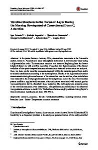
boundary layer and reported the presence of elongated streamwise strips of uniform low- and high-speed fluid (length > 8δ). Such elongated momentum regions were even noticed within the atmospheric surface layer studies of Young et al. [2002] and Drobinski et al. [2004]. In more recent studies of the near neutral atmospheric surface layer, Hutchins & Marusic [2007a], Marusic & Hutchins [2008] and Hutchins et al. [2012] observed large-scale u-fluctuations that are qualitatively similar to those found in laboratory experiments. Using the footprint of the superstructures at the wall (detected by a wall shear-stress sensor), Hutchins et al. [2011] studied the conditional structure of u-fluctuations associated with a large-scale skin friction event in a high Reynolds number turbulent boundary layer. Their conditional mean results showed the presence of forward leaning low-speed structures above a low skin-friction event, with regions of high momentum on either side of it (also shown in figure 2.8). Dennis & Nickels [2011], who used high-speed PIV in a boundary layer, provided invaluable information on the three-dimensional structure of the largest motions, consistent with Hutchins et al. [2011]. Thus far, we have discussed the evidence in support of the existence of large-scale structures in high Reynolds number flows. They have been observed universally

Literature Review

23

3 1.0

2

1z/δ 0.5 0 0.5

1 100 0

1y/δ

–0.5

10–1 10–2 10–3 0.5

1y/δ

0

1x/δ

–1 –2 0

–0.5

–3

Figure 2.8: Iso-contours of the streamwise velocity conditionally averaged on a low shear-stress event. Three-dimensional view of the x − y plane, x − z plane and three y − z planes at locations of x/δ = 0, 1 and 2. Two sets of graphs are presented, one set with linear scaling and the other with logarithmic scaling of the axis. From Hutchins et al. [2011].

in internal geometry flows (such as pipes and channels), in flat-plate turbulent boundary layers, in a supersonic boundary layer ([Ganapathisubramani et al., 2006]) and even in a near neutral atmospheric surface layer ([Hutchins & Marusic, 2007a]). In parallel to these studies, researchers have also studied the influence the large-scale structures exerted on the near-wall structures/skin-friction fluctuations. A summary of the developments in the understanding of inner-outer interactions in a boundary layer is presented in the following section.

2.2.1

Influence on the near-wall structures

First of all, we clearly distinguish the two types of influences, the large-scale structures in the outer layer have on the small-scale motions in the near wall region. They are, (1) superposition and (2) amplitude modulation. We refer to superposition, the phenomenon where the large-scale structures simply impose outerscaled energy onto the near-wall structures. This idea has been used to explain the increasing inner peak value of u2 with Reynolds number. With amplitude

Literature Review

24

modulation, we are referring to the dynamic amplification or attenuation of the small-scale fluctuations by the large-scale motions convecting in the log-region. Superposition Using a high-resolution Laser-Doppler anemometry, De Graaff & Eaton [2000] demonstrated that the magnitude of inner-normalised u2

+

is a strong function

of Reynolds number throughout the inner-region with exception to the sublayer. Through a comparison of results obtained using hot-wire anemometry across a range of Reynolds numbers, Metzger & Klewicki [2001] observed a logarithmic +

increase in the peak value of u2 when normalised using inner scales. They showed that the additional energy in the near wall u-fluctuations is contributed by the lowfrequency motions in the outer regions. Marusic & Kunkel [2003] proposed a similarity formulation to describe the streamwise turbulence intensity profile across the entire smooth-wall zero-pressure gradient turbulent boundary layer by considering physical arguments based on the attached-eddy hypothesis of Townsend [1976]. They also explained the increase in +

u2 at a fixed z + location is due to the presence of more and more eddies above +

the fixed location at high Re, and each of them contributing to u2 at the fixed z + location. Through their formulation, they suggested that the profile of u2

+

changes significantly with Reynolds number, with an outer flow influence felt all the way down to the viscous sublayer. Abe et al. [2004] analysed the instantaneous DNS data at Reτ = 640, and concluded that very large structures exist in the outer layer, and are visible in the instantaneous wall skin-friction fluctuations. Hutchins & Marusic [2007b] applied a simple Gaussian filter on the DNS database of del Alamo et al. [2004] and presented evidence that the ‘footprint’ of very long structures in the log-region is superimposed onto the near-wall cycle. Using the same argument, we can explain the observations of De Graaff & Eaton [2000], Metzger & Klewicki [2001] and Marusic & Kunkel [2003]. The increase in the magnitude of the inner-scaled peak in streamwise turbulence intensity can be explained as due to the increasing superposition of large-scale energy onto the near-wall region as Re increases.

Literature Review

25

Looking at the pre-multiplied energy spectra of streamwise velocity fluctuations at two Reynolds numbers (Reτ ≈ 1000 and 7300), Hutchins & Marusic [2007b] showed that there is an increasing amount of low wavenumber energy for the higher Reynolds number case and that this low wavenumber energy extends down to the wall. They also suggested that this phenomenon becomes increasingly prominent with increasing Reynolds number, as seen in the emergence of outer peak in the streamwise turbulence intensity. In the DNS data of a channel flow at Reτ = 2003, Hoyas & Jimenez [2006] explained the scaling failure in the peak value of the u based on the interaction of long and wide structures that are different than the near wall streaks. Amplitude modulation of small-scale events Using a hot wire in a turbulent boundary layer, Rao et al. [1971] studied the frequent periods of activity (termed ‘bursts’) in a band-pass filtered turbulent signal. They found that the characteristic time scale associated with these bursts scaled with outer variables δ and U∞ , indicating the dynamic interaction between the small-scales near the wall and the large-scale structures in the outer region. Through space-time correlations across the boundary layer, Blackwelder & Kovasznay [1972] reported an outward movement of the eddies along the trajectory of the bursts from the buffer layer, supporting the view point of Kline et al. [1967]. Based on these observations, they also suggested that the outer large-scale intermittent motions are definitely influencing the near-wall bursting phenomenon. Brown & Thomas [1977] used an array of hot wires and wall shear stress probes and observed that the passage of the large structure left a characteristic response in the region close to the wall. In their results, they observed that the wall shear stress has a slowly varying part and a high-frequency part and that the wall shear stress appears to be coupled with the δ-scale bulges in the outer layer. Bandyopadhyay & Hussain [1984] studied numerous shear flows, including boundary layers, mixing layers, wakes and jets, to understand the relationship between the large- and smallscales in such flows. Based on short time correlations between the low-frequency component of the u-velocity signal and a signal similar to the envelope of the

Literature Review

26

high-frequency component of the velocity signal, they observed strong coupling between scales in all flows. More recently, similar observations are noted by Hunt & Morrison [2000] in the atmospheric surface layer data. Instantaneous pictures of very large scale motions were shown by Iwamoto et al. [2005b] affecting the streamwise velocity fluctuations close to the wall in a DNS channel flow at Reτ = 2320. Furthermore, Ganapathisubramani et al. [2003] and Marusic & Hutchins [2006] both showed enhanced Reynolds shear-stress concentrations aligned within the elongated low-speed regions of the log layer. In a more recent study, Hutchins & Marusic [2007b] decomposed the velocity signal into large- and small-scales using a spectral cut-off filter (λ+ x = 7300) and observed that the large-scale motions caused amplification or attenuation of small-scale u, v, and w fluctuations. Using the conditional results of small-scale fluctuations, they showed that the low-speed structure consists of weakened smallscale energy close to the wall and this trend switches to a regime of more intense small-scale activity farther away from the wall. This interaction was quantified by Mathis et al. [2009a], and formed the basis of a successful algebraic model (abbreviated as the ‘inner-outer-interaction’ (IOI) model) by Marusic et al. [2010], wherein the statistics of the streamwise velocity fluctuations in the near-wall region could be predicted given only the large-scale information from the outer boundary layer region of a given flow. Mathis et al. [2009b] compared the phenomenon of amplitude modulation in three flows - pipe, channel and boundary layer and noted the amplitude modulation effect remains invariant in the inner region of all three flows, while some differences are observed in the outer region. Chung & McKeon [2010] investigated the statistics from large-eddy-simulation (LES) of turbulent channel flow at very high Reynolds numbers and reported findings that are consistent with the discussion in Mathis et al. [2009a]. Similar amplitude-modulation effects are noticed by Guala et al. [2011] in their hot-wire data obtained in the atmospheric surface layer. In addition, they noted that the envelope of instantaneous dissipation was also correlated with the large-scale ufluctuations across several wall-normal locations. Finally, Ganapathisubramani

Literature Review

27

et al. [2012] observed the phenomenon of frequency modulation by the large-scale events. They showed that the frequency is higher for positive large-scale fluctuations, and is lower for the negative large-scale fluctuations, noting that such an effect is largely limited to regions z + < 100. Within two years of the development of the IOI model, Mathis et al. [2013] applied it in the viscous sub-layer, where a linear relationship between the streamwise velocity and the wall shear-stress is known. They successfully implemented the model where the fluctuating wall shear-stress is reconstructed just by using the large-scale signal from the logarithmic region.

2.3

Turbulent skin-friction reduction techniques

The benefits of controlling turbulence are many considering the vast number of engineering applications where turbulent flows occur. Some of these benefits include drag-reduction, increased heat-transfer, reduced aero-acoustic noise and increased mixing. The associated economic benefits are too many to ignore the ongoing attempts of flow-control. However, the attempt to develop a control scheme which is energy-efficient and practical for a range of turbulent flows has been the most challenging. Organised motions are shown to play an important role in turbulent transport, see Cantwell [1981] and Robinson [1991]. Hence most attempts to control turbulent flows focussed on manipulating the coherent structures. Turbulence control methods can be classified into passive and active control. Passive approaches are those techniques in which a passive perturbation (steady forcing with no active feedback) is given to a boundary layer with the idea of suppressing or strengthening certain organised motions in the flow. With such techniques there is no feedback loop and their role is passive in that sense. On the other hand, in active control techniques, there is an active feedback either to minimise or maximise certain quantities of the flow, for example, skin-friction. Almost all flow control

Literature Review

28

schemes to date have targeted the near-wall cycle and there are very few techniques that have specifically targeted the large-scale structures. We here review some of the more successful techniques.

2.3.1

Large eddy break up systems (LEBUs)

The eddies in the boundary layer are linked to the bursting and entrainment processes that constitute the regenerative cycle of motions [Savill, 1979]. Several attempts were made in the past to perturb the dynamic cycle of turbulence production with the idea of reducing turbulence intensity and skin-friction drag. The methods mainly employed either reducing the burst events near the wall or suppressing the outer layer eddies. Early studies focused on breaking the large-scale eddies using devices called large eddy break-up systems (LEBUs) for the reasons that the perturbation would last longer in the streamwise direction. This work was initiated by Loerke & Nagib [1972], who employed the use of screens, grids and honey combs to reduce the free stream turbulence. Around the same time, Yajnik & Acharya [1977] developed flow management techniques based on the use of honeycombs and screens. They observed an huge reduction of up to 50% in the average skin-friction coefficient (Cf ) downstream of the screens. On the downside, these devices added pressure drag equivalent to an increase of 500% in Cf . An improvement to this scheme was made by Corke et al. [1979], where they implemented honeycomb like flat plate devices with a reduced number of horizontal members to reduce the device drag but nonetheless, affect a range of eddy structures and suppress production of turbulence in the flow. These experiments also inspired a parallel study carried out by Hefner et al. [1979]. In both these studies, they obtained a skin-friction reduction of about 20% but the associated device drag contributed to 50-90% increase in Cf .

Literature Review

29

Later studies investigated simpler geometries of these devices to optimise the overall benefit in reducing skin-friction integrated over certain downstream distance. Some of these attempts reported reductions ranging between 4 and 6% over a large streamwise distance ([Bertelrud et al., 1982], [Hefner et al., 1983]). However, in all these studies the reduction in drag has been calculated using indirect methods, momentum balance or wall-similarity velocity fits. And each of these techniques have their own limitations. Savill & Mumford [1988] conducted studies using floating-elements to measure the localised skin-friction in the flow modified by different configurations of flatplate manipulators. Also, they used flow-visualisation techniques to understand the interactions between the flat-plate devices with the eddies in the boundary layer. They suggested two possible mechanisms to explain the observed skinfriction reduction. The suppression of large-scale structures is one of these. The vortices generated by the flat-plate devices interact with the large-scale motions ensuring that the high momentum sweeps do not impinge on to the wall and thereby reduce Cf . A second mechanism was suggested based on the interaction between the vortices in the wake of these devices with the near wall structures. The vortices formed in the lower half of the wake of the devices counteracted the mean vorticity close to the wall and induced more upward motion of the hairpin vortex loops, thereby reducing the turbulent fluctuations and the mean velocity gradient near the wall. Anders [1989] summarised the different mechanisms that were proposed to explain how these devices reduced the skin-friction at the wall. Towards the end, he seems to indicate that the devices would not be effective at higher Reynolds number as the boundary layer structure is considerable different to that of low Re. To date, LEBUs remain one of the few attempts to control the large-scale structure in turbulent boundary layers.

Literature Review

2.3.2

30

Riblets

A riblet surface, is a surface with longitudinal micro-grooves that is used to obtain skin-friction drag reduction by modifying the near-wall coherent structures of the turbulent boundary layer. Walsh & Weinstein [1979] initiated the investigations of using a passive surface modification to achieve drag-reduction. Walsh [1983] and Walsh [1984] studied various types of riblet surfaces parametrically and found that the size of riblets should be of the order of the viscous-sublayer thickness in order to gain an overall drag reduction. In his experiments, Walsh [1983] reported a skinfriction reduction of about 8% and this has been confirmed by other experimental results from wind tunnel tests ([Choi et al., 1987]), from flight tests ([McLean et al., 1987]) and high-speed tunnel measurements ([Squire & Savill, 1987]). Different mechanisms were proposed to explain the turbulent drag reduction observed by using riblets. The first of these was given by Bacher & R. Smith [1986], who considered the interaction between the small eddies and the counter-rotating streamwise vortices near the peaks of riblets. They argued that the secondary vortices would lower the strength of the longitudinal vortices and also contain the low-speed fluid within the grooves. Choi [1984] tried to explain the mechanism in terms of the increased spanwise vorticity and the thickening of the viscous sublayer which is analogous to the case of drag-reducing polymers. A year later, Choi [1985] and Choi [1987] suggested that the hindrance to the spanwise movement of longitudinal vortices by the riblets is the prime reason for the observed turbulent drag reduction. In other words, they explain that the spanwise movement of the pair of vortices associated with the near-wall bursts is restricted by the riblets, resulting in a weak premature burst, thereby reducing the turbulent skin-friction. A similar mechanism was highlighted by Bechert et al. [1985] and Bechert et al. [1986] where they argued that the cross flow efficiency of the momentum transfer is impeded by the riblet ridges, thereby leading to a reduction of turbulent skin friction. From the results, they were able to conclude that the height by which the riblets protrude into the boundary-layer flow is of crucial importance in drag reduction.

Literature Review

31

Walsh [1989] concludes that the mechanism of skin-friction reduction by the riblets is closely related to the interaction with the near wall coherent structures as the effects were observed relatively close to the wall (usually y + < 30). He supports this view point stating that at these heights, only low-speed streaks and quasi-streamwise vortices constitute the coherent structures. Using the U-level technique, Baron & Quadrio [1997] also showed that the frequency of ejections increased by the presence of riblets. They concluded that the duration of the ejections decreased over the riblet surfaces compensating for the increased frequency of the events. It was generally perceived that in turbulent-flows, the drag increases dramatically with the increase in surface area owing to the shear stresses at the surface acting across the new, larger surface area. Based on this, questions were raised on the performance of riblet surfaces. Lee & Lee [2001] provided an explanation to this issue. They explained that the vortices that form above a riblet surface remain above them, interacting only with the tips of riblets. Since the higher speed vortices interact only with a small surface area at the riblet tips, only the localized area experienced high-shear stresses. Furthermore, it also means that they do not induce any high-speed flow in the valleys of the riblets. On the other hand, they allow a low-speed fluid flow in the valleys of the riblets leading to reduced levels of shear stress on major portions of the riblet surface. Against all these facts, there are number of practical complications to this method. For example, in the case of aircraft applications, fouling and degradation of the riblet surface can reduce its efficiency. The additional weight added to the aircraft and finally the lifespan of a riblet surface all play role in the success of their application. However, in the recent years all these problems have been addressed and riblets have been successfully applied in many practical applications. Competition swimsuits that are commercially sold use a thread-based riblet geometry. Drag reductions in riblet application have also been accomplished in flight applications and fuel savings as large as 3 per cent have been reported, see [Dean & Bhushan, 2010]. Research is being carried out in manufacturing riblets that are specific to the application.

Literature Review

2.3.3

32

Wall blowing and suction

Turbulent flow with wall blowing and suction has been investigated considerably over the past few decades. Wall blowing and suction have been applied either uniformly in space or locally through a thin slit over a limited spatial extent. The effect of wall suction on the coherent structures of a turbulent boundary layer has been studied by Antonia et al. [1988]. They observed a more orderly behaviour of low-speed streaks and a greater longitudinal coherence of the low-speed streaks from visualizations of a turbulent boundary layer with uniform suction. It was noted that the frequency of heating or cooling is reduced by suction, as seen from the decreased number of ejections in the flow visualization. They explained that suction reduces the breakdown of low-speed streaks, which results in reduced turbulence energy, Reynolds stresses, temperature variances and heat fluxes. Park & Choi [1999] carried out a DNS study to understand the effects of uniform blowing and suction on a turbulent boundary layer. In their simulation, they used a spanwise slot and used a magnitude of less than 10% of free stream for blowing and suction. They reported that in the case of uniform blowing, the skin friction reduced rapidly in the immediate downstream location of the slot. The near wall streamwise vortices are lifted up weakening the interaction of the vortices with the wall, and hence reducing the skin-friction. Following this, the lifted vortices became stronger as they travel downstream of the slot. This increased the turbulent velocity fluctuations and the skin-friction at locations further downstream of the slot. On the other hand, an opposite phenomena is observed in the case of uniform suction. In the immediate downstream location of the slot, there is a large increase in skin-friction. However, the near wall streamwise vortices are drawn closer to the wall, and are diffused due to viscous forces. This makes them weak as they advect downstream resulting in reduction in turbulence levels as well as the skin-friction at a further downstream location from the slot.

Literature Review

2.3.4

33

Spanwise wall oscillation

Through numerical simulations of a planar channel flow, Jung et al. [1992] indicated that spanwise wall oscillations at T + = 100 produced large reductions (40%) in the turbulent drag and also reduced the turbulence intensities of all three velocity components as well as the Reynolds shear stress. They also observed that the results are independent of whether the oscillations are caused by a cross-flow or by the physical motion of a channel wall. However, in the latter case, reduced turbulence is observed only at the oscillating wall, while the flow at the other wall remained fully turbulent. They suggested that the reduced turbulence is due to the decrease in the number of burst events in the oscillatory channel flow as compared to an unmodified flow. Experimental confirmation of these results was provided by Laadhari et al. [1994] for a low Reynolds number boundary layer flow. They explained that the decrease in skin-friction is due to the reduction in mean velocity gradient of the boundary layer near the oscillating wall. An experimental study by Choi et al. [1998] also showed a similar result of skin-friction reduction at slightly higher oscillation frequency. They suggested a mechanism by which the streamwise vortices are tilted towards the spanwise direction, thereby reducing the fluctuations in streamwise vorticity. Furthermore, they also suggested that the wall oscillation velocity is a more important parameter than oscillation frequency. This result was further corroborated by Choi & Graham [1998] in a pipe flow study. In their flow visualisation results, they observed that the meandering motion of the streaks is greatly reduced when the walls are oscillated in the spanwise direction. This resulted in a reduced spanwise vorticity and a reduced turbulence intensity. Based on the model proposed by Orlandi & Jimenez [1994] for skin-friction generation, Dhanak & Si [1999] inserted a counter-rotating vortex pair into a minimal channel. In their simulation, an oscillatory motion is applied to the channel walls and the downstream development of the vortices was analysed. They explained

Literature Review

34

the mechanism of skin-friction reduction as follows; during the spanwise oscillation, the cycle of near-wall turbulence production is disrupted which eventually reduces the rate of generation of the streamwise streaks. From an experimental study, Choi [2002] reported that both the duration and strength of the sweep events were greatly reduced over the oscillating wall, leading to a reduction in the skin-friction drag of up to 45%. They explained that the decrease in skin-friction is due to the reduction in the mean velocity gradient. They attributed negative spanwise vorticity (generated over the oscillating wall) as the reason for decreasing the velocity gradient close to the wall. The practical implementation of this approach is debatable. A great amount of power is required to physically oscillate the walls of an engineering system. A simple calculation was performed by Baron & Quadrio [1995] taking into consideration the overall energy balance and the power spent to oscillate the wall. In their simulation study of channel flow, they kept the frequency of oscillations constant at the most efficient value determined in previous studies (see Jung et al. [1992]). They observed that there is an overall benefit at smaller amplitude oscillations and on the other hand energy deficit is observed at higher amplitude oscillations. They also demonstrated that net energy savings are possible from this drag reduction technique when the wall-oscillation amplitude was less than a half of the free-stream velocity. Berger et al. [2000] experimented a more realistic technique by oscillating the flow instead of the channel walls. He simulated the Lorentz force (the force generated when a conducting fluid flow passes through a magnetic fluid) and observed similar results of 40% skin-friction reduction in their simulation, however the energy efficiency of such a scheme again turned out to be non promising.

2.3.5

Vortical flow

Schoppa & Hussain [1998] conducted a DNS study in a turbulent channel flow where they investigated a new large-scale control strategy to reduce the generation

Literature Review

35

of streamwise vortices by stabilising the low speed streaks. They investigated two types of forcing schemes; (i) counter rotating streamwise vortices, inserted at the centre line of the channel and (ii) spanwise colliding jets at the wall. In both these cases, they observed tremendous reduction in skin-friction; 20% using the counter rotating vortices and 50% using a wall jet control for a weak forcing. On the other hand, at high forcing magnitude, they observed increased drag. Based on this, they reported that the forcing strength should be chosen to be just strong enough to stabilise the near wall streaks for optimum control. In their simulation, they used a transverse wavelength of 400 wall units for the counter rotating vortex pair and observed the maximum effect at a surprisingly weak magnitude of 6% of the centre line velocity. Schoppa & Hussain [1998] explained that the drag reductions observed in the case of vortex control and wall jet control is due to weakening the longitudinal vortices close to the wall by suppressing the instability of the streaks. Following the perturbation scheme presented in the numerical simulation of Schoppa & Hussain [1998], an experimental study was carried out by Iuso et al. [2002]. They conducted experiments in a fully developed turbulent channel flow at Reτ = 180 and manipulated it using a spanwise array of vortex generator jets mounted along the upper wall of the channel. The jets are all circular in geometry with 2 mm diameter, placed 30 mm apart from each other and are mounted at an inclination of ±450 to the flow direction. The distance between the adjacent jets corresponded to about 3 times the half-channel height, and the net mass flow rate through the jets was about 3% of the channel mass flow rate. They used a high jet velocity about 5 times the centre-line velocity in the channel. Iuso et al. [2002] reported large reduction in the mean and fluctuating skinfriction. They attributed these results mainly to the induced flow by the counter rotating vortex pairs generated by the jets. When the induced flow is directed towards the wall, large reduction (∼ 50%) in skin-friction is observed. And in the regions where the cross-flow is fully developed, a reduction of 30% is noticed in skin-friction. They explained that the reductions observed in the mean and

Literature Review

36

variance of skin-friction are due to the stabilisation of the low-speed streaks by the forcing flow. Due to the weakening of the low-speed structures, they become less prominent in giving rise to new longitudinal vortices and in this manner, the strength of the turbulence regeneration cycle is reduced. Both these studies, [Schoppa & Hussain, 1998] and Iuso et al. [2002] attempted a passive control or a constant forcing on the flow. Moreover, the Reynolds number of their study is quite small and it is questioned whether such strategies still hold at higher Reynolds number flows. We take into account both these factors in the current study. We are here attempting the possibility of large-scale control in high Reynolds number turbulent boundary layer using an active control strategy.

2.3.6

Active control

For the first time, Choi et al. [1994] conducted numerical simulations and showed the possibility of reducing the skin-friction drag by manipulating the near wall structures. They investigated different types of control namely; normal velocity control, spanwise velocity control, streamwise velocity control, combined control and control with sensors at the wall. Choi et al. [1994] evaluated the efficiency of these different control schemes based on the change in the mean pressure-gradient required to drive the flow in a channel flow with a fixed mass flow rate. In the normal velocity control, a wall-normal velocity was imposed on the flow that is exactly opposite in direction but equal in magnitude to the wall-normal velocity component in the flow at a given y location in the boundary layer. They found that the optimal detection location yd+ is approximately 10. They reported skin-friction reduction up to 20-30% using either the normal or the spanwise velocity control techniques. An important result has been noted in the study of Choi et al. [1994]. Previously, it was known that uniform blowing increased the fluctuations and decreased the skin-friction and the opposite trend is observed in uniform suction. However, the study of Choi et al. [1994] showed that in active blowing reduced the skin-friction as well as the velocity fluctuations.

Literature Review

37

In the case of spanwise velocity control, Choi et al. [1994] applied an out-ofphase condition to the spanwise velocity to reduce the strength of streamwise vortices which increase the wall-normal velocity towards the wall. In this type of active control, they reported a drag reduction of about 30%. Based on closer observation of the simulation results, they proposed two different mechanisms to explain the drag reduction achieved using active control techniques. Firstly, they noted that the sweep motions are inhibited by the active control without disturbing the primary streamwise vortices. This behaviour was observed in a very short duration after the control is applied. Instead, the regions of high shear rate are pushed towards the interior of the channel. Secondly, the near wall vorticity layer is affected by the active control, preventing the lifting of spanwise vorticity. Consequently, the generation of streamwise vortices is reduced which lead to a reduction in skin-friction. Carlson & Lumley [1996] performed a numerical simulation of minimal turbulent channel flow where a Gaussian bump was used as the actuator for opposition control. They tried to obtain skin-friction reduction by raising the actuator whenever a sweep event was detected in the flow. Later, in a DNS study, Kang & Choi [2000] applied a local deformation to the wall using the opposition control methods highlighted in the study of Choi et al. [1994]. By doing so, they observed a drag reduction of 17%. They highlight that the deformed wall surface closely resembled that of riblets in appearance, however, pointed out that the mechanism is quite different from that of riblets. Iwamoto et al. [2005a] implemented a virtual active feedback control to reduce skin-friction drag by minimising the turbulent velocity fluctuations close to the wall, with the idea of studying the Reynolds number dependence of such schemes. They developed an expression for the drag reduction rate as a function of friction Reynolds number (Reτ ) by assuming that the velocity fluctuations below a certain wall-normal location are perfectly diminished to zero. Based on this, they suggested that if the turbulence below y + = 10 is counteracted by an active control, one can achieve a drag reduction of up to 35% even at high Reynolds number (Reτ ) = 105 . However, it has to be pointed out here that these results are only a

Literature Review

38

prediction from their derived expression for drag reduction rate. It is neither possible to simulate a flow at such high Reτ nor to implement such an active control in experiments in order to realise the truth of this statement. Furthermore, they have not considered the energy input to carry out such active control in real time, especially considering the fact that the small-scales become even smaller at high Re. A successful experimental study was carried out by Rebbeck & Choi [2001] demonstrating the possibility of reducing the skin-friction drag by inhibiting the downward motions of sweep events. However, their study was done off-line where the opposition control was simulated in a conditional sense. A few years later, Rathnasingham & Breuer [2003] used a linear active control scheme to affect the near wall region of a boundary layer. They used multiple sensors and a spanwise array of synthetic jets and constructed a feed-forward control. They reported reductions of up to 30% and 7% respectively, in the streamwise velocity fluctuations and the skin-friction. With improved instrumentation and better computing devices, Rebbeck & Choi [2006] revisited their original study [Rebbeck & Choi, 2001], and carried out a real-time wind tunnel measurement to specifically target the sweep events. They studied the modifications to the near wall structure under these conditions. In their study, they employed a combination of in-phase streamwise velocity and out-of-phase normal velocity control and reported that this combination showed an increased effectiveness of opposition control. A recent experimental study was carried out by Kang et al. [2008] where they applied an opposition control to counteract the rising hairpin vortices using a jet issued from a nozzle positioned outside the boundary layer. They analysed the results off-line where they correctly hit the hairpin with the jet. In their analysis they observed that there is a scope of reducing skin-friction by directly intervening the hairpin structures in the flow, however, the jet has to be properly scaled to the strength of the hairpin. They conclude with a note on the benefits of implementing a real-time control scheme to reduce the wind tunnel time for such experiments.

Literature Review

39

Most of the control schemes discussed so far only used wall-based techniques and hence are impractical in their application in high Re flows. This is because the time and length scales of the near wall structures reduce as the Reynolds number increases. To implement such active control methods in practical flows, it would need enormous number of sensor-actuator pairs. For instance, under cruising conditions for a passenger air plane, the streak spacing is around 100 wall units. This amounts to 0.1 mm which implies that every 1 m2 of fuselage requires O(108 ) sensor/actuator pairs. Nevertheless, the above studies bring out the potential of real-time control, if only the ideas of opposition control can be implemented on the large-scale structures in the flow.

2.4

Summary

Summing up the discussion from the previous section, it is very clear that there is a substantial scope for modifying the structure of a turbulent boundary layer. There have been a great many attempts at controlling the coherent structures in turbulent boundary layers, some successfully. However, most techniques seem to be limited in their application, due to the concern over their energy-efficiency. In many case, the amount of energy input to implement any of the control methods exceeds the energy saving due to skin-friction reduction, except in the case of riblets. Although riblets showed promising results, their practical application is met with problems arising due to the degradation of the riblet surface over time. The prospects of turbulence control shown by simulation studies are difficult to realise in real applications considering the energy input and the complexity of implementing such schemes. One reason for the lack of success of these methods is that most flow-control techniques are investigated in low Reynolds number flows, while in industrial practices, the flows are generally at high to very high Re. There is certainly a need for more high Reynolds number flow control studies. Adding to this, the mounting evidence for the existence and importance of large-scale structures and their

Literature Review

40

increasing influence at high Re on the wall-shear stress, turbulence intensity and Reynolds shear stress, suggests that these features could make an attractive target for future control schemes. At this point, we ask a question, “How about active control of large-scale motions ? ” The reasons why such techniques could be superior are: (i) the larger timescales available for such control schemes, (ii) requirement for fewer number of sensors/actuators and (iii) it is anticipated that a less intricate feed-back control is involved. Our attempt here is a step towards the goal of controlling the large-scale structures in high Reynolds number flows. Our study is quite different from previous studies in two fundamental aspects. Firstly, we are only targeting the large-scale structures in the flow at high Re and secondly, we are emulating a real-time active control. Based on this hypothesis, we first embarked on understanding and characterising the large-scale structures and their influence on the near-wall turbulence. The outcome of these experiments are used to build an off-line control scheme, which is later tested to effectively target the large-scale structures in a high Reynolds number flat-plate turbulent boundary layer. The results from our off-line study are presented in chapter 7. The motivation here is to look for the feasibility of using a wall-normal jet or any other large-forcing to actively target the large-scale structures. We here aim to obtain a parameter space that would be a useful input to future active control schemes. It should be noted that the overarching goal of this study is to further our understanding of large-scale structures when they are perturbed. This is an important precursor to more serious attempts at control of large-scale structures.

Chapter 3 Experimental set-up The Experimental set-up comprises of four sections:

• § 3.1 Facility • § 3.2 Constant temperature anemometry • § 3.3 Measurement stations • § 3.4 Jet actuator

3.1

Facility

The experiments are conducted in the open return High Reynolds Number Boundary layer Wind Tunnel(HRNBLWT), located in the Walter Basset Aerodynamics lab at the University of Melbourne. The HRNBLWT achieves high Reynolds numbers using the ‘big and slow’ approach by having a long working section and using moderate flow velocities. The test section has physical dimensions of 27 m length × 1.89 m width × 0.9 m height and its schematic is shown in figure 3.1. The long development length ensures that within a boundary layer under moderate free-stream velocities, high spatial and temporal resolution can be obtained with existing instrumentation. Throughout this study, we adopt a coordinate system 41

Experimental set-up

42

as shown in figure 3.1. We use x, y and z for the streamwise, spanwise and wallnormal directions respectively, and u, v and w represent the respective velocity fluctuations. Also, U refers to the time averaged mean velocity, u refers to the fluctuating velocity signal and uˆ is the total velocity. Careful considerations went into the design of this facility. The entrance to the tunnel is fitted with a bell mouth. This enables smooth entry of air flow, reduces acoustic noise and prevents any adverse pressure change across the entrance. This section leads to a heat exchanger that moderates the temperature to within ±0.1o C operating in a feedback loop. Data from two temperature sensors, one before the fan and a second one at the end of the tunnel working section is used in a feedback loop to maintain the flow temperature to within the above mentioned limits. Following the heat-exchanger, the rectangular cross section of the plenum gradually changes into a circular section through a transition chamber consisting of perspex and timber laminate panels mounted onto a hexagonal shaped skeleton. This provides a clear view of the fan driving the flow across the tunnel and also helps in inspection of the flow quality passing through the fan. The fan is driven by a computer controlled 200 kW DC motor, and the speed of the fan is controlled through a system implemented on a computer. Following the motor assembly, the tunnel takes a 1800 turn in two stages, consisting of a pair of curved vanes, a settling chamber consisting of a honeycomb flow-straightener and a series of six fine mesh screens to make the flow uniform. The flow, then enters a contraction section with an area reduction ratio of 6.2:1. With all the meshes and contraction section, a good flow quality is achieved in √ this tunnel. The free-stream turbulence intensity, defined as u2 /U∞ , is nominally 0.15% (at the test section located nominally 21 m from the start of the working section) for a free-stream velocity range of U∞ ≈ 20-40 m/s. Here, u2 is the mean variance and U∞ is the free-stream velocity. For the current study, a free-stream velocity of 20 m/s is used. With this free-stream velocity a friction Reynolds number Reτ defined as, Reτ = δUτ /ν ≈ 15000 is achieved. Here, δ is the boundary layer thickness, Uτ is the mean friction velocity and ν is the kinematic viscosity

Air bleeding slot

Honey comb & series of meshes Contraction (6.2:1)

Experimental set-up

Turning vanes

0.92m

1.89m

Trip 27m working section Axial Fan

z

y

Heat exchanger

Plenum mouth

x Bell mouth

Drag Balance

43

Figure 3.1: Three dimensional sketch of the Wind Tunnel Facility

Experimental set-up of the working fluid. The mean friction velocity Uτ is defined as, Uτ = where τw is the shear-stress at the wall and ρ is the density of the fluid.

44 p

τw /ρ,

The flow is tripped at the entrance to the working section by a coarse grade P40 grit sand paper. The specifications of the trip have been discussed in the thesis work of Kulandaivelu [2012]. This facility has a fixed floor and an adjustable roof that consists of 22 rectangular panels each of dimensions 1.2 m length × 0.9 m width on either side of the centre line of the tunnel. A nominally zero pressure gradient is achieved by adjusting the height of these panels and varying the bleeding gaps between the adjacent panels. The gap between two sections of the roof (on either side of the tunnel axis), is sealed by a series of brush seals, which not only provide a good seal but also facilitate the stream-wise movement of the traverse. All the inner side edges of the tunnel have fillets to prevent any formation of corner vortices. A thorough study of pressure gradient in the streamwise and spanwise directions is presented by Kulandaivelu [2012]. This tunnel is fitted with several state-of-art instruments to acquire data. The details of the test section used in this study in this facility are discussed in the following.

3.1.1

Test section

The test section used in this study refers to a section of the wind tunnel that is between streamwise distances, x = 19.5 m and x = 22.5 m from the trip. It is an interchangeable floor section that is 2.7 m in length and 0.7 m in width. The test-section floor is fitted with either a smooth and flat Aluminium sheet or a transparent glass surface that provides optical access to the flow. Such a design facilitated the use of multiple experimental techniques such as Hot-Wire Anemometry (HWA) and Particle Image Velocimetry (PIV). This would enable a direct comparison of the results obtained using these two methods. For the current study, this section is made of nine rectangular flush-mounted Aluminium plates, each of dimensions 0.3 m × 0.7 m. These nine plates cover a length of 2.7 m in the stream-wise direction, as shown in figure 3.2. Each of these tiles have been machined to a reference height so that the resulting surface roughness is within

Experimental set-up

45 Traversing system

Pitot-static tube

Traversing hot-wire probe Two spanwise arrays of skin-friction sensors

2.7m

Flow

0.7 m

Nine plates assembled to replace the central section of drag plate

Rectangular Jet

Figure 3.2: A schematic drawing of all the sensors and actuators used in this study

the hydrodynamic roughness less than 3.5 wall units. These plates are supported from the bottom using two L-shaped brackets mounted to the tunnel floor along the length of the test section. Any unevenness arising due to the use of multiple tiles is further adjusted using fine-threaded screws at four corners of these tiles. By adjusting the fine-thread screws, the plates can be moved up or down in small increments giving us a better resolution and ability to control the flatness and unevenness of the plates.

3.1.2

Wall-normal Traverse

The traversing system used in the HRNBLWT facility is a fully automated system, designed to facilitate hot-wire anemometry measurements in a turbulent boundary layer at any streamwise station along the length of the tunnel. To this end, it is built to have a two-axis movement in the streamwise (x) and wall-normal (z) directions. A schematic of the traverse is shown in figure 3.3 and a cut-open section is also shown giving the details of linear encoder and the bull-screw rod. It is fitted with two servo motors, each controlling its movement in one direction. In the streamwise direction, a pulley and a belt mechanism is used to drive a platform

Ball screw

Experimental set-up

Parallel rails - Wall normal movement Roof

Gold strip Read-head Pitot tube Position Encoder

0.5 m Hot-wire Probe holder Wall surface


Pneumatic
cylinder

10o

0.55 m

Retractable Pneumatic foot

46

Figure 3.3: Two axis traverse assembly

Experimental set-up

47

that rests on a pair of parallel cylindrical rails, running through the length of the wind tunnel. This platform holds all the measuring equipment and is driven by a servo motor with a gear assembly ratio of 60:1. In the wall normal direction, a ball-screw rod is driven by a second servo motor with Renishaw RGH24-type linear encoder system providing real-time feedback to the servo motor. It has a resolution of 0.5 µm in wall-normal direction. The shape of the traverse is designed to resemble an aerofoil to reduce blockage effects and vortex shedding. It has a chord length of 18 cm and a width of 3 cm, closely resembling a NACA0016 profile. Kulandaivelu [2012] studied the blockage caused by the traverse system in this facility as a part of calibrating the entire facility. He concluded that the blockage is negligible with the variation in freestream velocity to within ±0.3% when the measuring probe is ±0.5 m from the leading edge of the traverse. A unique feature of this traverse is its capability to self-contain all the cables running from various sensors mounted to it. Such an arrangement minimizes any flow disturbances that would have been otherwise caused by cables hanging on the outside surface of a traversing system. Another unique feature of the traverse is its retractable foot system. When positioning at a station, the foot is pneumatically actuated with compressed air at approximately 30 psi pressure providing the rigidity to the traverse even when the tunnel is operated at very high speeds. The foot is additionally held strong by a vacuum pump that constantly provides a suction from the lower side of the foot. The traverse also houses a Pitot-static tube, temperature and an atmospheric pressure sensor. The Pitot-static tube shown as a component in figure 3.3, is in-house built and calibrated against the standard Pitot-tube supplied by the National Physics Laboratory (NPL), UK. It is built as a straight type with brass to a length of 0.5 m. The wall-normal position of the Pitot-static tube is selected so that it is well outside the boundary layer and within the free-stream potential flow. It is to be noted here that the boundary layer thickness is of the order of 0.35-0.4 m towards the end of the working section of the wind tunnel and hence the Pitot-static tube is mounted at a height of 0.52 m above the tunnel floor. The atmospheric pressure sensor is a

Experimental set-up

48

144S-PCB model from SensorTechnics, USA to be used in an atmosphere of either dry air or dry gases and has operating temperatures of −45o C to 85o C. This sensor is mounted on the platform that rests on the parallel cylindrical rails along with other equipment. Finally, the temperature sensor is a DP25 series thermocouple from Omega, USA that can operate between 0o C to 60o C with an accuracy of ±0.5o C. Typically average temperatures range between 200 C to 300 C at different times of the year.

3.2

Constant temperature anemometry

The sensors used in these measurements are two spanwise arrays of flush mounted skin-friction sensors and a traversing hot-wire probe as shown in figure 3.4. Various measurements have been carried out using a combination of these sensors. The configuration of these sensors and their frequency characteristics are discussed in the following sections.

3.2.1

Traversing hot-wire probe

A single hot-wire is mounted to the traversing system with the sensing element 550 mm upstream of the leading edge of the traverse. The probe is a boundary layer type Dantec 55P15 hot-wire probe and has a prong spacing of 1 mm with Platinum-Wollaston wire soldered to the prong-tips. The wire diameter is d, the etched length of the wire is l and the length-to-diameter ratio is l/d. In the current study, a wire diameter of 2.5 µm with an etched length of 0.5 mm is used to achieve an l/d ratio of 200, as recommended by Ligrani & Bradshaw [1987] and Hutchins et al. [2009]. Full details of the hot-wire probe are shown in figure 3.5. The sensor length(l), normalised by inner length scale (ν/Uτ ) is denoted by l+ . The superscript + is used to denote viscous scaling of length (e.g. l+ = lUτ /ν), velocities (U + = U/Uτ ) and time (t+ = tUτ2 /ν). The non-dimensional sample interval is given by t+ (= tUτ2 /ν, where t = 1/fs and fs is the sampling frequency).

Experimental set-up

49

The total length in seconds of the velocity sample at each wall-normal position is given by T . This is non-dimensionalised by outer scaling to obtain the boundary layer turnover time T U∞ /δ. For converged statistics the boundary layer turnover time number needs to be several thousands of the largest scales in the flow as recommended by Hutchins et al. [2009]. The non-dimensional sampling interval and the boundary layer turnover times for different experiments are summarised in table 3.3 along with other mean flow quantities. The hot-wire probe is operated in Constant Temperature Anemometry (CTA) mode using an in-house Melbourne University Constant Temperature Anemometer (MUCTA) with an overheat ratio of 1.8. The indicated frequency response of the hot-wire probe to a 1 kHz internal pulse is about 25 kHz. The hot-wire signal is sampled using a Data Translation 16-bit data-acquisition board. For the experiments reported here, measurements are made at 40 logarithmically spaced points between 0.3 6 z 6 500 mm in the wall-normal direction.

Flow

∆xD hfd Jet

hfu Figure 3.4: Schematic drawing of the experimental set-up. The two spanwise arrays of skin-friction sensors are denoted by hfu and hfd , and the distance between them is represented by ∆xD .

Experimental set-up

50

0.5mm

Figure 3.5: Specifications of hot-wire used in this study. The wire diameter (d) is 2.5 µm and the etched length is 0.5 mm.

To carry out calibration, the traversing hot-wire probe is positioned at z = 500 mm, which is in the potential flow region beyond the edge of the boundary layer. It is calibrated against the Pitot-static tube before and after every experiment, referred to as pre- and post-calibrations. The free-stream velocity is varied from 0 m/s to 23 m/s and the mean voltages of the hot-wire are recorded as a function of free-stream velocity (U∞ ). A total of 12 calibration points are used during pre- and post-calibrations. During any given boundary layer traverse experiment, after every five measurement points in the boundary layer, the traversing probe is moved to z = 0.52 m and the voltage of the hot-wire in the free-stream flow is logged. This helps in tracking any drift in the hot-wire voltage and can be used to correct for the drift. A very elaborate discussion on the strength of this approach has been provided by Kulandaivelu [2012]. In short, this method involves generating multiple calibration curves by using the drift in hot-wire voltage to shift the pre- or post-calibration curves.

3.2.2

Cross-wire probe

In chapter 4 of this work, the conditional structure of the three velocity components in a three dimensional space is characterised. To compute this, measurements are taken using a multiple hot-wire sensor system, also termed ‘cross-wire probe’. Two

Experimental set-up

rements show clear scale sepa-

0.4 (l x ) 0.2 (∆sz ) 0.4 (ly ) Platinum wire

10◦

15 10 z (mm)

ise and spanwise fluctuating ved in a high Reynolds number turcustom made sub-miniature hot e made over a range of Reynolds 500, but at fixed unit is the kineis the boundary he measurement volumes of the 7 viscous esolved velocity measurements, ends in isolation from spatial res-

51

5 0

✂

✂ ✂

✍✂ ✂

Ceramic housing Stainless steel prong 30 20 x (mm) 10

Dantec compatible connection Epoxy 60 50

40

−5 ectra for both components show 20 −2 in viscous units and an outer re0 y (mm) , which grows in magnitude with ths associated with the outer site Figure 3.6: Custom built cross-wire An exploded viewfigure) of the prong tips Figure 1: (main figure) Customprobe; cross-wire probe, (inset is shown in the inset figure, with cuboid volume of 0.4 × 0.4 × 0.2 mm shown overlaid. All dimensions in mm. From Baidya et al. [2012].

different configurations are used here; (1) a uv probe to measure simultaneous streamwise and spanwise velocities, and (2) a uw probe to obtain synchronised streamwise and wall-normal velocity measurements. A cross-wire probe in general is a combination of two single hot-wire probes with an inclination of ±45o to the flow direction. In the current study, a miniature cross-wire probe of dimensions 0.4 × 0.4 × 0.4 mm has been used (developed and built at the University of Melbourne, see [Baidya et al., 2012]). Figure 3.6 shows a schematic of the cross-wire probe that measures the streamwise and spanwise velocities. Various dimensions of the probe volume are illustrated in the figure. Here, lx , ly and ∆sz represent the three dimensions of the cuboid that can enclose the sensor volume. The non-dimensional dimensions for both uv and uw cross-wire probes are listed in table 3.1. The motivation behind this new probe is the non-availability of commercial cross-wire probe systems smaller than 1.2 × 1.2 × 1.2 mm. Each single wire in a cross-wire probe has a diameter of 2.5 µm and its etched length is maintained to have l/d > 200, according to recommendations of Ligrani & Bradshaw [1987].

Experimental set-up

52

Type of CW probe

lx+

ly+ /lz+

+ ∆s+ z /∆sy

uv uw

17 17

17 17

8.5 8.5

Table 3.1: Normalised dimensions of sensor lengths of the cross-wire probe.

Since a moderately high Reynolds number flow is used for this study, the probes are designed small enough to have a viscous scaled sensor length of approximately 22 (l+ = 22), to have sufficiently resolved velocity measurements. The crosswire probe is operated using a constant temperature anemometer in the same procedure, used for a single hot-wire sensor. The only difference is the over heat ratio; for a cross-wire probe, a lower overheat ratio of 1.6 is used whereas a ratio of 1.8 is used for the single normal hot-wire. This slightly lower value is chosen to minimise the thermal cross-talk between the closely spaced sensors. The calibration of cross-wire probe is performed in situ to remove the need to relocate the probe between the calibration rig and the sting. The calibration rig consists of a jet mounted on a two axis traversing system allowing rotation along the pitch and yaw axes. For the calibration of the wires measuring streamwise and wall-normal velocities, the probe is placed at the axis of rotation and the jet is pitched using a stepper motor about the spanwise axis. An encoder affixed to the axis provides an accurate measurement of angle of the jet relative to the wire. At each velocity of the jet, 11 pitch angles are used between −30o to +30o . The corresponding voltages from wire 1 and 2 (E1 and E2) are recorded to build a voltage to velocity conversion map. A similar procedure is used to calibrate a cross-wire probe that measures the streamwise and spanwise velocities. More details of the calibration procedure are given in Baidya et al. [2012].

Experimental set-up

53

0.026 m

0.9 mm

Spanwise array

Figure 3.7: Specifications of spanwise array of skin-friction sensors.

3.2.3

Hot-film sensors

Arrays of flush-mounted skin-friction sensors are affixed to two of the nine tiles (discussed in section 3.1.1). The upstream and downstream skin-friction sensor arrays are hereafter referred to using hfu and hfd respectively. Each of the spanwise arrays consists of nine skin-friction sensors, as shown in figure 3.7. They extend to a length of ≈ 0.72δ in the spanwise direction (y), with a spanwise spacing of 0.026 m or 0.08δ. Here the notation hfu1→9 and hfd1→9 refer to each of the 9 individual skin-friction sensors on the upstream and the downstream arrays respectively. These arrays are separated by a streamwise distance ∆xD , defined as the distance between the hfu and hfd arrays. By varying the distance ∆xD , it is possible to study the effect of increasing separation on the streamwise correlation of large-scale structures in the flow (see figure 3.2). The hot-film sensors are Dantec 55R47 glue-on-type sensors, operated in a CTA mode using AA labs AN1003 anemometer with an overheat ratio (OHR) set to 1.05. The sensors are numbered from 1 to 9 as shown in 3.7. All the sensors were R 495. Each sensor is made of a nickel film with glued to the wall using Loctite

dimensions (0.1 mm × 0.09 mm) coated on an insulating polyamide foil. The foil has a thickness of 50 µm causing a wall normal step of ∼ 50 µm (due to its thickness and affixing tapes). In the current facility this height only corresponds to a step height of approximately 3.3 viscous units and thus considered hydro-dynamically

Properties

Array

Sensor

Type

Upstream spanwise array

hfu1 hfu2 hfu3 hfu4 hfu5 hfu6 hfu7 hfu8 hfu9

55R47 55R47 55R47 55R47 55R47 55R47 55R47 55R47 55R47

20.4 20.4 20.4 20.4 20.4 20.4 20.4 20.4 20.4

-0.104 -0.078 -0.052 -0.026 0 0.026 0.052 0.078 0.104

75 75 75 75 75 75 75 75 75

0.9 0.9 0.9 0.9 0.9 0.9 0.9 0.9 0.9

39 39 39 39 39 39 39 39 39

-

-

1.05 1.05 1.05 1.05 1.05 1.05 1.05 1.05 1.05

Downstream spanwise array

hfd1 hfd2 hfd3 hfd4 hfd5 hfd6 hfd7 hfd8 hfd9

55R47 55R47 55R47 55R47 55R47 55R47 55R47 55R47 55R47

21 21 21 21 21 21 21 21 21

-0.104 -0.078 -0.052 -0.026 0 0.026 0.052 0.078 0.104

75 75 75 75 75 75 75 75 75

0.9 0.9 0.9 0.9 0.9 0.9 0.9 0.9 0.9

39 39 39 39 39 39 39 39 39

-

-

1.05 1.05 1.05 1.05 1.05 1.05 1.05 1.05 1.05

hw

55P15

21

0

z

0.5

22

2.5

200

1.8

l+

d (µm)

l/d

OHR

54

Traversing probe

−→ z l (µm) mm

Experimental set-up

Location y (m)

←− x (m)

Table 3.2: Dimensions and positions of all the sensors

Experimental set-up

55

smooth (see for example, Shockling et al. [2006] who showed no roughness effects for roughness height less than ∼ 3.5 wall units). The precise locations of the spanwise skin-friction sensors and the hot-wire can be found in table 3.2 The hot-film sensors are simultaneously calibrated during the hot-wire calibration process. The mean voltages are obtained from each of the hot-film sensors as a function of free-stream velocity (U∞ ). Using a known empirical formulation between Uτ and U∞ given by Chauhan et al. [2013], it is possible to fit a third order polynomial between the mean voltages of hot-films and Uτ values. Furthermore, these sensors are calibrated after every five wall-normal measurements in a similar manner to that of the hot-wire. Due to a low overheat ratio (OHR), it is noticed that the hot-film sensors have pronounced drift issues. However, their drift pattern between the pre- and post-calibrations has been observed to be linear and with the use of intermediate calibration voltages, the drift is accounted for. Throughout this work, the data from the skin-friction sensors are used only for detecting the passage of large-scale events. Hence, any error in the calibration process will have minimal impact on the analysis presented in the later chapters.

3.2.4

Single and two-point correlations: hot-wire and hotfilm sensors

The hot-film sensors are only used as a detector of the large-scale events and their effectiveness has been discussed at length by Hutchins et al. [2011]. Here in our study we note that the correlation results closely resemble those of Hutchins et al. [2011]. However, in this study the sensors are glued to the surface (unlike in the study of Hutchins et al. [2011] where the sensors were taped), and we noticed a reduced magnitude of peak correlations. Figure 3.8 shows the cross correlation of the skin-friction fluctuations across one of the spanwise arrays,

Ruτ uτ (i, j) =

(uτhf i uτhf j ) σ(uτhf i )σ(uτhf j )

(3.1)

Experimental set-up

56

1 0.8

Ruτ uτ

0.6 0.4 0.2 0 −0.6

−0.4

−0.2

0

0.2

0.4

0.6

∆y/δ

.

Figure 3.8: Two-point correlation of measured skin-friction fluctuations between: (+) hf4 and all other sensors, (◦) between hf5 and all other sensors and (·) all sensors in the spanwise array.

where i and j are the sensor numbers 1 to 9 of either of the arrays. Also, uτhf i is the fluctuating friction velocity as measured by sensor i in one of the spanwise arrays and σ is the standard deviation of the signal. The plus symbols show the correlation between hfu4 with all other sensors (i =4, j =1:9), the circle symbols show the correlation between hfu5 with all other sensors (i =5, j =1:9) and the solid dot shows the correlation between all the other sensors. Both the spanwise arrays of sensors exhibit similar behaviour. The result also suggests that all nine sensors are behaving in a consistent manner and the shape of the correlation curve is consistent with previous experimental studies of ? and Monty et al. [2007]. The positive peak and the negative trough are separated by approximately 0.35δ in the figure 3.8, which is a well-known characteristic of large-scale events away from the wall, also highlighted by Schlatter et al. [2009]. Further analysis is carried out to determine how these sensors respond to the large-scale structures in the streamwise direction. This gives a measure of the temporal response of the skin-friction sensors. Figure 3.9 shows the autocorrelation of the skin-friction fluctuations of the middle sensor of the hfd array defined as, Ruτ uτ (i, ∆t)|hfd5 =

uτ (t)uτ (t + ∆t) . σuτ σuτ

(3.2)

Experimental set-up

57

1 0.8

Ruu

0.6 0.4 0.2 0 −80

−60

−40

−20

0

20

40

60

80

∆t (milli-seconds)

.

Figure 3.9: Comparison of auto-correlation curves of a skin-friction sensor with a hot-wire positioned directly above it at z + = 8. The solid line is for the skin-friction sensor, the dashed line is for the hot-wire and the dot-dashed line is for the hot-wire signal, filtered using a box filter at a frequency of 400Hz.

This is compared with the auto-correlation curve of a hot-wire placed directly above the sensor hfd5 . The solid line shows the autocorrelation of sensor hfd5 and the dashed line shows the autocorrelation curve of the hot-wire. It can be inferred that the hot-wire is able to capture the high frequency content of the signal while the hot-film sensor is merely limited to resolving only the low frequencies. This can be understood more clearly by a comparison between the auto-correlation curves of the hot-film signal and the filtered hot-wire signal, which is also shown in figure 3.9. The dotted line shows the autocorrelation curve of the hot-wire signal filtered using a box filter at a frequency of 400 Hz (equivalent ∆t of 2.5 milliseconds). The collapse of the auto-correlation curve of the filtered hot-wire signal to that of the hot-film sensor suggests that the hot-film sensors are not resolving energy above ≈ 400 Hz.

3.2.5

Filtering of hot-film signals

In this study, our prime focus is the very large-scale motions in the flow and their footprint which is identified using the hot-film sensors. On this basis, the time-series signals of the hot-film sensors are filtered using a Gaussian filter with

Experimental set-up

58

Filtering - Gaussian filter

1δ

Figure 3.10: Process of filtering the signal of a skin-friction sensor. A time series signal is filtered using a Gaussian filter of length 1δ to obtain the detection signal for this study

standard deviation σ = δ/6 (also corresponds to a filter length of 1δ for a Gaussian filter), as explained in figure 3.10. The zero-mean time series signal is passed through a Gaussian filter and the resultant signal represents only the signature of larger scales. The filter length has been determined to effectively isolate the very large-scale motions from the hot-film signals. By inspection, it is clear that the residual signal is a true representation of the large-scales in the flow.

3.3

Measurement stations

A second series of experiments are carried out using a combination of the two arrays of skin-friction sensors, traversing hot-wire probe and a jet actuator. To understand the downstream evolution of the large-scale structures in this study, measurements are carried out at different streamwise locations by varying ∆xD between the two sensor arrays hfu and hfd . Several comparisons are made in later chapters between these stations and in order to present the results in a coherent manner, a nomenclature of these stations is developed. Each station is referred

Experimental set-up

59

to by a notation sn where n represents the number of tiles (discussed in section 3.1.1) between the hfu and hfd arrays. Figure 3.11 shows the streamwise locations of all the measurement stations. Here, distances are measured from the reference station s0, where hfu is mounted, and are shown in two scales; (1) physical units of metres and (2) normalised units of δ. These stations extend over a streamwise length of 7δ to facilitate the study of evolution of large-scale structures in the streamwise direction. At each of these measurement stations, velocity measurements were made in a rectangular grid that is log-spaced in the wall-normal direction and uniformly spaced in the spanwise direction. This type of measurement grid is used to obtain greater resolution close to the wall. For the conditional analysis, the sensor hfu5 (marked as a red dot) is used as the detection sensor or the conditioning point. All the mean flow parameters have been obtained by fitting the composite profile of Chauhan et al. [2009] with log-law constants, κ = 0.384 and A= 4.17. It is noticed that boundary layer thickness so obtained, is 15% higher than the value reported by Hutchins et al. [2011] who obtained it using the modified Coles wake fit of Perry et al. [2002] on measurements from the same facility. Nonetheless, this variation in δ using different velocity fits does not alter the results presented in this work as the boundary layer thickness is only used as a scaling parameter (outer normalisation factor). Other integral parameters such as displacement thickness (δ ∗ ) and momentum thickness (θ) along with the Reynolds numbers defined based on them are listed in table 3.3. Here, Reynolds numbers defined based on δ ∗ and θ are Reδ∗ = U∞ δ ∗ /ν and Reθ = U∞ θ/ν respectively . Looking at the tabulated values of δ across different measurement stations, it is evident that it does not change significantly over the test section of the tunnel used in this study. This is clearly seen in figure 3.12 where the variation of δ is plotted against streamwise distance. This result justifies the use of a single value of δ for normalising the results when comparisons are made at particular free-stream velocity. The boundary thickness at station s0, denoted as δ0 , is chosen as the

s7 .

0.3

0.75

∆z/δ

−0.3 1

s5 .

0.5

0.5 ∆z/δ

s4 .

0.25 0

0

∆y/δ

0

s3 . −0.3

0

∆y/δ

2.1

s2 .

0.3

6

1.5 5

1.2

∆z(m)

0.4

0.9

0.2

∆y(m)

7

1.8

s0 .

0 0.1

∆x(m) 3

0.6

4

∆x/δ

2

0.3 0 −0.1

Experimental set-up

1

1

0 0

60

Figure 3.11: Schematic drawing of all measurement stations used in this study. The dimensions are shown in metres and also in the normalised units of δ. The tiles that make up the test section are shown in grey lines on the plane (z = 0). A full-sized measurement grid is shown in the inset picture.

Experimental set-up

Station

x (m)

Reτ

Reδ∗

Reθ

δ (m)

δ∗ (m)

θ (m)

+ S(U∞ )

ν/Uτ (µm)

l+

t+

T U∞ /δ

s0 s2 s3 s4 s5 s7

19.83 20.43 20.73 21.03 21.33 21.93

14984 15692 15999 15197 15549 16010

47372 50982 53037 51526 51813 53294

37079 39841 41379 40054 40374 41888

0.369 0.378 0.381 0.369 0.381 0.385

0.0376 0.0392 0.0401 0.0396 0.0404 0.0409

0.0294 0.0307 0.0313 0.0308 0.0315 0.0321

31.06 31.35 31.52 31.53 31.48 31.33

24.6 24.1 23.8 24.2 24.5 24.0

24 23 23 23 25 24

1.32 1.33 1.34 1.31 1.3 1.32

39201 38213 38009 39127 37752 37428

Table 3.3: Mean flow properties based on the parametric fit of the composite velocity profile of Chauhan et al. [2009] for different measurement stations. The notations s0 → s7 represent the stations at which the measurements were carried out.

61

Experimental set-up

62 .

0.5

s0

s2

s3

s4

s5

20.4

20.7

21

21.3

s7

δ (m)

0.4 0.3 0.2 0.1 0

19.8

20.1

21.6

21.9

x (m) Figure 3.12: Variation of boundary layer thickness (δ) across the streamwise locations of the stations s0 → s7. The dotted line shows the reference boundary layer thickness (δ0 ) which is used as the outer normalising length scale in this study.

common outer length scale and hereafter, δ refers to the δ0 . A similar trend has been observed in the change of Uτ with streamwise distance.

3.4

Wall-normal jet

The jet used in this study is a rectangular slot of dimensions 50 mm×2 mm giving an aspect ratio of 25:1. It is mounted 0.3 m downstream of the hfu array with its centre positioned at a streamwise distance of 20.13 m from the trip. A schematic of the jet used in this study is shown in figure 3.13. The manifold is a box which consists of ten tubes that are arranged in a zig-zag fashion to obtain a rectangular cross section of the exit plane of the jet. A compressed air reservoir feeds the pneumatic line, characterised by a regulator valve that allows the jet mass flow rate to be changed. A static port on the side wall of the jet is used to monitor the exit velocity of the jet. Care has been taken to see that the profile of the air column exiting the rectangular slot is uniform across the length. Both Pitot-static tube measurements and single hot-wire measurements are carried out to study the time response of the jet assembly and also to establish the uniform flow pattern.

Experimental set-up

Solenoid valve

63

✲

Static port

❥

Figure 3.13: Wall-normal jet assembled to a rectangular plate. Top view of the jet is shown in the inset picture.

3.4.1

Characteristics of jet

The jet velocity used in this study is 10 m/s, while the free-stream velocity is maintained at 20 m/s, giving a velocity ratio (Vr ) of 0.5. Velocity ratio is defined as the ratio of jet velocity to the free-stream velocity as, Vr =

Vj . U∞

(3.3)

A velocity ratio of 0.5 is used throughout this study. Based on the hydraulic diameter Dh = ≈ 4 mm, calculated as Dh = 4*Area/Perimeter, the Reynolds

Experimental set-up

64

number ReDh defined as,

ReDh =

ρUDh , µ

(3.4)

is approximately 4000 for this study.

3.4.2

Jet duty cycle

A square wave pulse, as shown in figure 3.14 is used to trigger the jet in a periodic manner to simulate an off-line control study. The control signal, hereafter referred to using j, is a binary signal of zeros and ones. The duty cycle time is the total time of the square wave while the actuation time is the duration for which the jet is turned on. In this study, a duty cycle time of 0.4 seconds and an actuation time of 0.1 second is used to facilitate conditional average studies based on jet actuation. The reasoning behind choosing an actuation time of 0.1 s is explained here. In a flow with free stream velocity of 20 m/s, the large scale structures are convecting at a speed (Uc ) of 14 m/s [Hutchins et al., 2011]. This means that if the jet is actuated for 0.1 s, it would be able to affect large-structures that are of the length 0.1 × Uc = 0.1 × 14 ≈ 3δ in our wind tunnel facility. Moreover, since the actuation time is only 25% of the duty cycle, the flow recovers to a canonical state during the jet-off period.

3.4.3

Evolution of jet into the boundary layer

The first characteristic of the jet we want to study is its penetration depth into the boundary layer developing over it. To understand this, a series of measurements were taken at five streamwise locations, upstream and downstream of the jet, when the jet is continuously actuated. These measurement stations are denoted by letters a, b, c, d and e at streamwise locations (in metres) of 20.08, 20.11, 20.13, 20.15 and 20.205 respectively. The velocity of the jet has been set at 10 m/s, giving a velocity ratio of 0.5. In these measurements, only a single hot-wire probe

Jet signal(Volts)

Experimental set-up

65

1 ON

OFF

0

0

0.2

0.4

0.6

0.8

1

Duration of Jet signal(sec)

Figure 3.14: Specifications of duty cycle of the Jet

is used to resolve the magnitude of velocity. However, since these experiments are primarily carried out to understand the penetration depth of the jet, a single hot-wire was sufficient.

a

b

c

d e

35 30

U 25 Uτ 20 15 10 20.08

x(m)

10 20.11

3

20.13

10 20.15 20.205

10

2

zUτ ν

Figure 3.15: Mean velocity profiles during a continuously pulsed jet, at different streamwise locations, upstream and downstream of the location of the jet.

4

Experimental set-up

66

The results from these experiments are presented in a three dimensional view, in figure 3.15. Along the x direction, the streamwise locations of the jet (drawn as blue coloured box) and the measurement planes are shown. The wall-normal direction is shown along the y axis and finally the normalised mean velocity is plotted along the z-direction. This kind of representation is useful for representing both the penetration depth of the jet and its downstream evolution. For the normalisation, we use the viscous length and velocity scales, where Uτ is obtained at a location upstream of the jet. The mean profile at location a shows no effect of the jet, confirming no upstream effect of the jet. Thus the mean quantities at this station have been used to normalise other quantities. It is clearly evident that the jet has affected the mean profiles at measurement planes (b-e) above and downstream of the jet. We can see that the jet is able to penetrate deeper as it is convected downstream, and settles at an approximate wall-normal location (z + ≈ 750 or z/δ = 0.06) once it has reached the streamwise location at station(e). This is also confirmed in other measurements (not shown here) taken at locations downstream of station(e). From all these results, we observed that the jet penetrates well into the logarithmic regions of a turbulent boundary layer, where the large-scale structures are known to inhabit, for example, see Marusic et al. [2010], Ganapathisubramani et al. [2003], Hutchins & Marusic [2007b] and Guala et al. [2011]. Thus, it proved to us that the strength and geometry of the jet is sufficient to attempt to target the large-scale structures convecting at some height from the wall surface.

3.4.4

Spanwise movement of the jet

For the results discussed in chapter 6, various experiments were conducted by using a spanwise array of hot-film sensors, a rake of three hot-wires and a jet. Such a configuration of sensors is required in order to study the simultaneous effects caused by the jet in the spanwise direction. This can be done by moving either the hot-wire or the jet to different spanwise locations.

Experimental set-up

67

φ70mm 50mm×2mm

Flow 0.3m

0.7m

Figure 3.16: Schematic drawing of the plate holding the rectangular Jet. Tiles shown in the inset are two possible orientations leading to two spanwise positions for the jet.

In our study, we chose to fix the hot-wire probe and move the jet to various spanwise locations, in increments of 26 mm, which is equal to the separation between the two adjacent hot-film sensors. To facilitate these different configurations for the jet, a plate has been built with a rectangular cut section, as shown in figure 3.16. This plate (dimensions - 0.3 m × 0.7 m) is one of the nine plates, discussed in a previous section, that fill the central test section. An additional tile, smaller in size, that fits into the rectangular cut section of the bigger plate, holds the entire jet assembly. The circular section signifies the outer dimensions of the jet assembly and the rectangular slot is the jet. Here, it is possible to position the smaller tile in two ways with respect to the flowdirection, thereby achieving two different spanwise positions for the jet. This is also explained in the schematic drawing of the plate, where a second position for the smaller tile, is achieved by rotating the previous orientation by 180 degrees. Furthermore, within the small tile, the jet can be mounted in two orientations,

Experimental set-up

68

one along the streamwise direction and the other along the spanwise axis, as illustrated in figure 3.17. In this way, this experimental set-up can be used to study the spanwise effects of a wall-normal jet oriented in the streamwise and the spanwise directions.

Flow

Figure 3.17: Schematic drawing of the tiles used to obtain streamwise and spanwise orientations of the jet.

Chapter 4 Skin-friction measurements using drag balance This chapter describes the skin-friction measurement with the use of a floating element. The technique relies on accurately measuring the shear force exerted by a moving fluid on a large floating surface. The results essentially prove the ability of a novel facility at the University of Melbourne in measuring the integrated skinfriction force. This forms the basis of its usage to conduct future drag reduction studies at high Reynolds number flows. The results obtained from this facility have been previously published in the Proceedings of 17th Australasian Fluid Mechanics Conference 2010 (Talluru et al. [2010]). Here, that presentation is repeated with additional material included. The results are presented in a manner that is consistent with the remaining chapters of the thesis. A point to note here is that this facility will be used to test the final capability of any real-time control schemes. The current thesis concentrates on preliminary experiments, which investigate such control schemes using conditional off-line approaches. As such, the drag balance is not used at this stage. However, in the future this facility will play a key role as these proposed schemes are implemented in real-time.

69

Skin-friction Measurement

4.1

70

Introduction

Wall-shear stress, or skin-friction, is the local tangential force per unit area exerted on a body as a result of fluid flow over it. The shear stress is manifested through the ‘boundary layer’ which exists as a consequence of the no-slip condition at the wall and is the region of high shear between the wall and the outer free-stream flow. Of fundamental importance to this problem is the need to understand the behaviour of the wall-shear stress, denoted by τw . The accurate measurement of τw has long been a challenge. Techniques used for measuring wall shear stress may be categorised into two main groups; (i) the indirect methods and (ii) direct methods. The indirect methods are the techniques where the information of τw is inferred from another quantity in the flow. These methods make inherent assumptions about the flow to obtain a relationship between τw and the measured quantity. Hence, they require accurate calibration and are susceptible to errors. Examples of these methods include, Clause-chart, Von-Karman momentum integral method, viscous sublayer profile and Preston-tube technique. On the other hand, direct methods measure the wall shear stress . Hence no prior assumptions are made about the flow. These techniques are superior to the indirect methods. The floating element method and oil-film interferometry are the primary techniques that fall into the category of direct methods. Most indirect techniques, that have been used so far suffer from limitation in their applicability. The most prominent method used is the Clauser-chart [Clauser, 1954], wherein, Cf is obtained by fitting the logarithmic velocity profile to the measured mean velocity [Mori et al., 2009]. It inherently assumes the existence of a universal law of the wall (a logarithmic profile for the mean velocity). However, the indication from other direct measurements of Uτ , was that the constants that describe the logarithmic profile differed from their accepted values [Nagib & Chauhan, 2007].

Skin-friction Measurement

71

Another commonly used method involves using the K´arm´an integral momentum equation [Nagib et al., 2007] by calculating the development of momentum thickness downstream based on the relation Cf ≃ dθ/dx (for a ZPG turbulent boundary layer). This needs very detailed stream-wise development measurements and differentiation of experimental data which is prone to errors. In addition, this method is sensitive to weak pressure gradients and any residual three-dimensionality that exists in nominally two-dimensional, zero-pressure gradient test sections [Savill & Mumford, 1988]. The third method of obtaining Cf is to find the mean velocity gradient close to the wall, τw = µ(dU/dy)y→0 [Mori et al., 2009]. This method is challenging due to the difficulty in making measurements very close to the wall, with conduction and blockage issues for hot-wires and correction schemes required for Pitot tubes [Hutchins & Choi, 2002]. On the other hand, wall shear stress can also be determined by direct methods independent of the velocity profile. Floating element drag balance and oil-film interferometry are the primary techniques of achieving this [Winter, 1977]. Recent advances enable us to obtain more accurate results using these methods [Ruedi & Monkewitz, 2003]. These include extensive experimental analysis on floating element devices by Osaka & Mochizuki [2003] to measure local skin-friction resistance in a zero-pressure gradient boundary layer and the work by Nagib et al. [2007] and Osterlund et al. [2000] in improving the oil film technique. Many previous studies with a floating-plate drag balance as reported by Savill & Mumford [1988] rely on local skin-friction cf measurements. The problem with these measurements is that they do not account for the parasitic drag or any other additional form drag associated with the floating element design. One of the problems most small wind tunnel facilities face is the small viscous length scale ν/Uτ at high Reynolds number measurements. Due to small value of ν/Uτ at high Re, any unevenness on the floor would result in hydrodynamic roughness greater than the acceptable value. Typically any unevenness should be limited to within 3ν/Uτ (approximate hydrodynamic smoothness). To avoid such problems and obtain large values of ν/Uτ , wind tunnels are operated at low speeds. However, this leads to another problem. Due to smaller free stream velocity, only a very

Skin-friction Measurement

72

low Uτ value is obtained in the measurements. Thus, we are faced with time-series data, where the magnitude of signal is comparable to the noise levels, making it very difficult to distinguish between the two. All these problems are overcome in the present large-scale facility (HRNBLWT), a schematic of which is shown in figure 3.1 of chapter 3. This facility is designed for the experimental study of high Reynolds number boundary layers. The working section of the HRNBLWT has a cross section of 2m width and 1m height, and is 27 m in length. It is built to have a long development length and low free stream velocities to obtain high Re without having a very small ν/Uτ . Furthermore, the long working section allows the boundary layer to grow over a long distance giving a thick boundary layer. The boundary layer near the working section of the drag balance is approximately 350 mm thick and is 20 m downstream from the trip, this provides a very good spatial resolution for measurements [Nickels et al., 2005].

4.2

Drag balance

The drag balance is a large flat plate of dimensions 3 m×1 m, mounted between streamwise positions 19.5 m and 22.5 m of the tunnel floor. The outer section of the drag plate is made of aluminium and the support structure is made from steel. The facility has an interchangeable central section, of either glass (providing optical access) or an aluminium plate to accommodate various smooth wall boundary layer experiments. The plate freely floats with the aid of four air bearings, a labyrinth seal and the span-wise locking system. Figure 4.1 shows a three dimensional CAD model of the entire assembly highlighting the key components. Firstly, the air bearing system which keeps the entire drag plate floating, is pneumatically driven at a pressure of 80 psi. The working principle of the airbearing system is explained in figure 4.2 where an expanded view of the air-bearing assembly is shown. Compressed air is fed into the air inlet valve which is then split into four other air ports. The air flows through slots in a maze fashion that is precisely machined on the stainless steel block. This essentially redistributes

Skin-friction Measurement

73

the compressed air and maintains a uniform pressure applied to the bottom side of the glass plate. Due to this a very thin layer of air [O(µm)] is formed between the glass pads and the supporting surface of the drag plate that is mounted to the floor of the tunnel. This mechanism supports the weight of the plate and also makes it virtually frictionless. Furthermore, to ensure that the mechanism works effectively, the drag plate was adjusted to remain horizontal with reference to a highly sensitive spirit level. By this we make sure that the weight of the drag plate itself does not contribute to the force measurement. The circumference of the drag plate consists of a gap which separates it from

Labyrinth seals Air bearing mechanism Ai

Span !"#$ lock mechanism

Load cell

Figure 4.1: Three dimensional CAD model of drag balance, with all the individual components. Streamwise movement

Spanwise movement

Glass surface

Stainless steel blocks with precisely machined pathway

The path of the arrows show the flow of compressed air

Direction of Airflow Compressed air inlet

Figure 4.2: Expanded view of air-bearing assembly with all its subcomponents. The flow-path of the compressed air is shown by the arrows on the right side of the figure.

Skin-friction Measurement

74

U-shaped metal block rigidly fixed to the tunnel surface Three screws holding the rectangular slab to the square metal block

Slotted square metal block fixed to the drag plate

Flow of compressed air

Air bearing system

Streamwise movement No spanwise movement

Figure 4.3: Expanded view of the spanwise lock assembly with all its subcomponents.

the rest of the floor of the tunnel. It is essential for the drag balance to perform accurately that no air escapes from this gap and there is no sudden step change in the tunnel floor as it would cause a pressure drop. Allen [1977] showed that there are significant errors in skin-friction measurements for higher values of h/δ, where ‘h’ is the misalignment height. However, due to the large size of the drag plate and a boundary layer thickness of approximately 350 mm this facility is less susceptible to these drawbacks with previous drag balance designs. Additionally to be certain that no air can escape, a labyrinth seal (shown in figure 4.1) is used around the circumference of the drag plate to ensure no physical contact between the drag plate and the tunnel floor, nevertheless, providing a complete seal. The third component of the assembly is the span-wise locking system shown in figure 4.3. This is also pneumatically driven and it prevents the plate from moving in the span-wise direction while still facilitating stream-wise displacement. The design is explained as follows. An U-shaped metal block is firmly attached to the tunnel surface. It holds a pair of cylindrical blocks through which the compressed air is fed into the system. The pressurised air creates a thin air-film between the circular pads and the rectangular metal block which can only move in the streamwise direction. A slotted square metal block holds the rectangular block firmly with the use of three grub screws. The slotted square block is rigidly

Skin-friction Measurement

75

mounted to the bottom surface of the drag balance. Two of such systems are mounted on the opposite diagonal ends of the drag balance. Thus, the spanwise movement of drag balance is arrested so that the entire design is only sensitive to the streamwise component of wall shear stress. Finally, the last component of the drag balance is a high resolution (O(20 mN)) load cell that measures very small forces. The load cell has a measuring range between 0 and 10 N force and it is mounted to one end of the drag balance as shown in figure 4.1.

4.3

Calibration

The load cell is calibrated to obtain the relation between the measured voltage and the applied force. To make a proper calibration, the force transducer has to be tested in situ, i.e. connected to the plate in its usual state and secondly the force applied has to be determined very accurately by an alternate method. Here, a mass and a pulley system is adopted as the calibration technique. The entire set-up used for calibrating the load cell is shown in figure 4.4. When a taut string slides round a peg, friction causes the tension to vary along the string. If the string is perfectly flexible, the friction limiting as described by Amonton’s law, the tensions T1 and T2 on the tauter and slacker sides respectively are related to φ, the angular displacement of the string, and to µs , the coefficient of static friction, by the Capstan equation [Stuart, 1961],

T1 = eµs φ . T2

(4.1)

The angular displacement of the string can be thought of as the angle spun by the length of the string which is in contact with the pulley. Using this technique, the coefficient of friction is obtained in a procedure that is described below. The results of the variation in T1 and T2 are plotted for three different values of φ (π/2, 5π/2 and 9π/2). Here T1 corresponds to measured value on the load cell and T2 refers to the applied force. For the same measured

Skin-friction Measurement

76 Threaded rod used to transfer the loads

Load cell Plate fixed to the tunnel surface

Plate fixed to the drag plate assembly

Ceramic bearing used as a pulley Fishing tie used as inextensible string

Weights hung at this end during calibration

Figure 4.4: A schematic of the set-up used for in situ calibration of the load cell.

4 Case1 - φ = π/2 radians

3.5

Force measured (N) - load cell

Case2 - φ = 5π/2 radians Case3 - φ = 9π/2 radians

3

2.5

2

1.5

1

0.5

0 0

0.5

1

1.5

2

2.5

3

3.5

4

Force Applied, Fx (N)

Figure 4.5: Measured force value on the load cell against applied force

value on the force transducer, we have different values of applied force due to the variation of φ. By substituting the values of φ in equation 4.1, one can estimate the coefficient of friction. In our calibration set-up, a low friction ceramic bearing is used as a pulley and

Skin-friction Measurement

77

the experiment is conducted in the same procedure as explained above. Figure 4.5 shows the plots of the three cases. It is observed that all the three cases collapsed very well, implying a very small static friction coefficient between the pulley and the string. The value of µs is obtained from these results and is found to be smaller than 0.004. This indicates that the ceramic bearing can be treated similar to an ideal pulley. Furthermore, a linear relationship between the applied and measured forces is noticed in figure 4.5, supporting the point further. A small deviation of (∼ 0.02) from a slope value of 1, is only observed for loads greater than 4 N.

4.4

Frequency response of drag plate

The main objective of the drag plate is to provide accurate measurements of the mean wall shear stress and hence the time response of the system becomes relevant for very low frequency changes (of the order of 0.01 Hz) [Sadr & Klewicki, 2000] in the mean flow. Because of this, it is necessary to determine the natural frequency response of the drag plate. This is done by analysing the response of the system to an impulse force. The drag balance is given short duration forces and the response from the load cell is recorded. Analysing the force signal we obtained the natural frequency close to 1.0 Hz. The frequency response of the system is also shown in figure 4.6. The original motivation of this facility was mainly to carry out drag reduction studies and measure the change in τw , i.e. ∆τw . It was designed to contain within itself all measuring instruments, the control circuitry to conduct real-time drag minimisation strategies and an on-board power source. However, due to its design we can also use the same facility to measure τw over a large surface. This is justified by the fact that the variation of skin-friction coefficient Cf over the length of the drag plate is approximately linear over the working section, and hence the average signal of Cf can be measured and compared to those obtained at the centre position of the drag plate. This is confirmed in figure 4.7 where the average Cf has been calculated using the K´arm´an-Schoenherr relation [Nagib et al., 2007] and

Skin-friction Measurement

78





1DWXUDO IUHTXHQF\ RI+]

í



+DUPRQLFV RIQDWXUDO IUHTXHQF\

í

Cornkvwfg



+] IURPSRZHU VRXUFH

í

í



í



í



í



í















Htgswgpe{‚)J|*

Figure 4.6: Natural frequency of drag balance. The harmonics are also shown in the figure.

is compared to a linear approximation across the drag plate. The corresponding streamwise positions were then obtained for both equations. With a linear fit, the x position is obtained as 21.000 m while using the K´arm´an-Schoenherr equation, it is found to be 20.973 m, which corresponds to a negligible difference in Cf . This allows us to compare the experimental data with measurements conducted at 21 m by Hutchins et al. [2009]. Details of the drag balance design, components and measurements at HRNBLWT are presented in the remainder of this chapter.

4.5

Results and discussion

The experiments were carried out at zero-pressure gradient (ZPG) in the HRNBLWT, located in the Walter Basset Aerodynamics Laboratory at the University of Melbourne. The free stream velocity U∞ , determined by a Pitot-static tube, was varied from 10 m/s to 20 m/s, yielding a Reynolds number range of Rex = 1.4 − 2.8 × 107 . The experiment had two objectives: firstly to determine how

Skin-friction Measurement

79

2.08 K´arm´an-Schoenherr

2.075

linear fit 2.07 x = 21.000 m (Linear fit )

cf × 103

2.065 2.06 2.055 2.05 x = 20.973 m K´arm´an-Schoenherr

2.045 2.04 2.035 33000

34000

35000

36000

37000

Reθ Figure 4.7: Comparison of Cf obtained using K´ arm´ an-Schoenherr fit and linear fit, in Reθ range obtained over the length of drag plate at the free stream velocity of U∞ = 20 m/s

the drag balance would function in the tunnel, and secondly to investigate and compare the average wall shear stress with prior results obtained by Hutchins et al. [2009] for similar Reynolds numbers in the HRNBLWT and other empirical equations given in the literature [Nagib et al., 2007]. Data was collected at each speed in two steps: initial pre-load on the force transducer with no-flow conditions, followed by force measurement with flow over the plate. Figure 4.8 shows a typical unfiltered signal from the force transducer during a sampling time of 60 seconds. In each of the stages, measurements were taken for a duration of over 180 seconds and the mean was calculated. The drag force on the plate was obtained as the difference of the two values from which τw can be calculated. τw can be used to determine Cf and Uτ using

Skin-friction Measurement

80

406 405

Hqteg‚)P*

404 403 4 30; 30: 309 2

42

62

82

Ucornkpi‚vkog‚)u*

:2

322

Figure 4.8: Typical unfiltered force signal from the transducer over a period of 100 seconds for U∞ ≃ 24 m/s

Cf =

τw , 1 2 ρU∞ 2

(4.2)

τw . ρ

(4.3)

Uτ =

r

To establish the reliability of the measurements from the drag balance facility, experiments were conducted several times and the averaged data with error limits, is compared with those as reported by Hutchins et al. [2009]. Results are shown in figure 4.9 and table 4.1, it can be seen that the experimental results closely match with previous findings with a maximum percentage difference of approximately 0.95%. Hutchins et al. [2009] obtained Uτ using Clauser chart method where logarithmic law constants of κ = 0.41 and A = 5.0 were used. The skinfriction coefficient cf , obtained from the drag measurements data is also plotted against Reθ in figure 4.10. These are compared with the empirical relations for Cf

Skin-friction Measurement

81

0.7 Experimental data1

0.65

Experimental data2 0.6

Experimental data3 Hutchins et al(2009)

Uτ (m/s)

0.55 0.5 0.45 0.4 0.35

8

10

12

14

16

18

20

22

U∞ (m/s)

Figure 4.9: Comparison of Uτ with U∞ from the drag-balance with Clauser chart results of Hutchins et al. [2009]

U∞ (m/s) 10.06 13.00 20.02

Uτ ([Hutchins et al., 2009]) Uτ (Drag Balance) (m/s) (m/s) 0.3398 0.4277 0.6376

0.3422 0.4237 0.6383

Absolute % difference 0.68 0.95 0.10

Table 4.1: Comparison of Uτ data with Hutchins et al. [2009]

mentioned in Nagib et al. [2007]. Reynolds number is calculated as Rex = U∞ x/ν, where x is the streamwise distance from the trip to the centre of the drag plate. Reθ is obtained from Rex by the relationship given by Nagib et al. [2007],

Reθ = 0.01277Re0.8659 . x

(4.4)

Skin-friction Measurement

82

3.6 Nikuradse Schultz-Grunow Prandlt-Schlichting

3.2

Schlichting fit Prandtl-K´arm´an White 2.8

cf × 103

K´arm´an-Schoenherr 1/7 power law 1/5 power law

2.4

Coles-Fernholz George-Castillo (1997) Experimental data

2

1.6

0

10000

20000

30000

40000

50000

60000

Reθ

Figure 4.10: Comparison of Cf values with established empirical relations for Cf with Reθ [Nagib et al., 2007]

4.6

Summary and conclusions

A unique drag balance facility has been built for the study of skin-friction in high Reynolds number wall turbulence. The facility is tested in the HRNBLWT facility at the University of Melbourne, to obtain direct measurements of skin-friction over a large surface. The approach employed the use of a drag balance, however, here the implementation is unique in two aspects, (i) the design and (ii) the Reynolds number at which the experiments were conducted. Measurements of skin-friction coefficient Cf at different Reynolds numbers are obtained. The system achieved the desired force measurements at various speeds and is able to continuously measure the mean wall shear stress over a sampling period of five minutes without any drift in the measurements. The results are compared with those obtained using a Clauser-chart method from the previous laboratory results conducted by Hutchins et al. [2009] at HRNBLWT. Comparisons are also made with various empirical relations for Cf available in literature.

Skin-friction Measurement

83

The concurrence of the results with the existing empirical relations and the experimental data suggest that the drag balance can be used with great reliability to obtain direct measurements of wall shear-stress. It also provides a greater scope for conducting various other skin-friction reduction studies on this facility.

Chapter 5 Three-dimensional conditional view of large-scale structures in the log-region A combination of cross-wire probes (uv and uw) and an array of flush-mounted skin-friction sensors is used to study the three dimensional conditional organization of large-scale structures in a high Reynolds number turbulent boundary layer. The current study is an extension of the previous work carried out by Hutchins et al. [2011]; analysing the conditional average maps and the amplitude modulation of small-scale fluctuations. However, here we report results based on all three components of velocity. The results are significant in two distinct ways, providing deeper insights into the dynamics of the large-scale structures; (1) they show that small-scale v, w and h−uwi are modulated in a very similar manner to that of u, and (2) they demonstrate the existence of roll-modes associated with the superstructure events. These have not been shown previously for laboratory data at high Reynolds numbers. A physical interpretation is attempted towards the end of the chapter by relating the organisational features of large-scale structures in the flow.

84

3D Conditional structure

85

The work presented in this chapter is a combined effort with one of my colleagues, Rio Baidya, at the University of Melbourne. Our contribution in building the experimental set-up and in collecting the data is equal. My colleague’s role is primarily building the sub-miniature cross-wire probes, while my contribution is assembling the array of skin-friction sensors and computing the conditional results on various quantities.

5.1

Background

Over the past few decades, significant research has been undertaken to understand large scale coherence in turbulent boundary layers, especially in high Reynolds number flows. The origin of this dates back to the findings of Blackwelder & Kovasznay [1972], who observed elongated regions of uniform streamwise momentum from the streamwise velocity fluctuations. Over the last decade, numerous studies using techniques such as hot-wire anemometry, Direct Numerical Simulations (DNS) and Particle Image Velocimetry (PIV), have substantiated the spatial and temporal nature of these large structures. PIV studies by Tomkins & Adrian [2003] have revealed the spatial nature of these structures in the instantaneous fields of streamwise velocity. Hutchins & Marusic [2007a] used a rake of hot-wires and from the time series data reported that these structures extend to large streamwise lengths and substantially meander in the spanwise direction. In addition, they also identified that these large scale structures maintain a footprint at the wall. This was explored by Hutchins et al. [2011], who used the large-scale skinfriction footprint at the wall to obtain a three dimensional conditionally averaged view of the large-scale superstructures in a turbulent boundary layer, while also investigating how these features modulate the small-scale fluctuations near the wall. Their study, however, solely employed measurements of streamwise velocity which limited their characterisation of the large-scale modulating events. Several studies have also investigated the wider spanwise organisation of the very large-scale structures. [?] identified counter rotating roll-like structures associated

3D Conditional structure

86

with the largest scale events using a DNS channel flow database (Reτ = 950). From high speed PIV measurements, Dennis & Nickels [2011] computed various conditional averages and showed a similar organisation in the spanwise vicinity of large-scale structures. Such a phenomenon was also observed in the atmospheric boundary layer studies (Marusic & Hutchins [2008]; Hutchins et al. [2012]). They reported such features not just in the conditional average maps but also in the instantaneous velocity vector fields in the spanwise wall-normal planes. Here, we extend the current understanding of these superstructures by measuring all the three velocity components individually associated with these events. Such analysis provides a more detailed picture of the large-scale motions and their interactions with the near wall turbulent motions.

5.2

Validation of sub-miniature cross-wire probe

The first step towards computing various conditional averages of the velocity components, is to validate the statistics obtained from the custom-built cross-wire probe. The specifications of the cross-wire probe have been discussed in detail in the description of the experimental set-up in chapter 3. Furthermore, the calibration procedures of cross-wires have been delineated clearly in Baidya et al. [2012]. A short note on the calibration procedure is also presented in chapter 3 of this work. In the present study, we have conducted measurements using uv and uw crosswire probes along with an array of skin-friction sensors in two different experiments. The experimental conditions of these experiments are listed in table 5.1. In the post-processing stage, various statistics and conditional averages are computed and are discussed in the following sections. The mean velocity and the turbulence intensity profiles of streamwise velocity from the two measurements (uv and uw) are compared against the single hotwire measurements of Hutchins et al. [2011] at a matched Reynolds number in the same wind tunnel facility, as shown in figure 5.1. It is clear from the figure that

3D Conditional structure

Probe Reτ type uw uv

Reθ

87

U∞ ν/Uτ (m/s) (µm)

14984 37079 19.0 15068 38379 19.5

24.6 24.8

+ U∞

δ (m)

θ (m)

0.369 0.373

0.0294 31.06 0.0304 31.06

t+

T U∞ /δ

0.496 30895 0.50 31336

Table 5.1: Mean flow properties based on the parametric fit of the composite velocity profile of Chauhan et al. [2009] for different cross-wire configurations.

there is a very good collapse of the mean and turbulence intensity profiles and any discrepancy observed is within the experimental errors. The non-dimensional sensing length (l+ ) used in this study is about 17 while the study of Hutchins et al. [2011] employed an l+ value of 22. Measurements were only taken above z + = 20 in the case of uw probe as permitted by the cross-wire probe geometry. A good agreement in the turbulence intensity profiles, as seen in figure 5.1(b), implies that the measurements have adequate spatial resolution, see Hutchins et al. [2009]. However, it is not entirely clear if the same is true in measuring the v and w fluctuations. In the case of statistics obtained from v and w components, there is no direct comparison due to lack of availability of statistics with a similar spatial resolution at the high Reynolds number considered in the current study. Hence, they are validated against the DNS data of Schlatter et al. [2009], albeit at lower Reynolds numbers (Reτ = 1271) and also against the turbulence intensity formulations given in Perry et al. [2002] and Kunkel & Marusic [2006] using the attachededdy hypothesis of Townsend [1976]. All the comparisons are shown in figure 5.2 (a-c). Overall, the results show a good agreement considering the difficulty in taking such measurements. They also seem to exhibit a consistent Reynolds number trend in comparison with the low Reynolds number DNS data. However, we noticed increased levels of turbulence intensity in v and w close to the wall (z + < 30) and reduced values in the logarithmic region.

3D Conditional structure

(a)

88

−3

35

−2

10

10

z/δ

−1

0

10

10

30

U+

25 20 15 10 5 (b)

10 8

u2

+

6 4 2 0

1

10

2

10

3

z+

10

4

10

Figure 5.1: Comparison of statistical quantities of streamwise velocity at U∞ ≈ 20 m/s and Reτ ≈ 15000; (a) Mean and (b) Turbulence intensity. The solid line shows data of Hutchins et al. [2011], symbols (# and ∗) respectively show the experimental results from uv and uw cross-wire probes.

3D Conditional structure

89

−3

4

10

−2

z/δ

10

−1

0

10

10

v 2+

3 2 1 0

w2+

1.5

1

0.5

0

−uw+

1

0.5

0

1

10

2

10

z+

3

10

4

10

Figure 5.2: Comparison of (a) Spanwise variance (b) Wall-normal variance and (c) Mean Reynolds shear stress. The solid line is DNS data at Reτ = 1271 (Schlatter et al. [2009]), the dashed line shows the formulations of Perry et al. [2002] and Kunkel & Marusic [2006]. The symbol (#) shows the experimental results from the cross-wire probes uv and uw.

3D Conditional structure

5.3

90

Three dimensional conditional view

The three dimensional structure of the superstructures can be studied by computing various conditional quantities from the uv and uw probes when the reference hot-film sensor meets a given condition. The signal from the skin-friction sensor is used to detect the structures convecting above it. Firstly, the signals from the skin-friction sensors are filtered using a Gaussian filter of length 1δ to isolate only the large-scale signature of the flow. From such a signal, a high skin-friction event is identified when the instantaneous skin-friction fluctuation is greater than zero and conversely, a low skin-friction event is detected when the fluctuation goes below zero. At these instances when a low or high skin-friction event is detected by a reference skin-friction sensor, an ensemble average of the hot-wire measured velocity fluctuations is computed within the boundary layer. The traversing cross-wire signal is conditionally sampled on the occurrence of a low or high friction event at each of the nine spanwise skin-friction sensors, enabling us to build a volumetric view of the conditionally averaged velocity fluctuations associated with the event. The conditionally averaged velocity fluctuations based on a positive skin-friction excursion (u|h ) can be defined as

u|h (∆τ, ∆y, z) = hu(t, y, z) | uτ (t − ∆τ, y − ∆y) ≥ 0i.

(5.1)

Here, ∆τ is the time-shift applied between the hot-wire and the hot-film signals, while ∆y and z are the spanwise and wall-normal distances between the two sensors. In these equations, u can be replaced by any of the three normalised-velocity fluctuations and uτ is the fluctuating friction velocity signal. The hot-wire and hot-film signals are time-series data and can be converted into spatial data by using Taylor’s hypothesis as x = −Uc t. Uc is the convection velocity of the largescale events taken to be Uc = 13.25 m/s (determined from the time-shift in the cross-correlation of the skin-friction sensors, discussed more elaborately in chapter 6). For a low skin-friction event, the ensemble averaged velocity fluctuation is defined as,

3D Conditional structure

u|l (∆x, ∆y, z) = hu(x, y, z) | uτ (x − ∆x, y − ∆y) < 0i,

91

(5.2)

and for a high shear-stress event, it is evaluated as, u|h (∆x, ∆y, z) = hu(x, y, z) | uτ (x − ∆x, y − ∆y) ≥ 0i.

(5.3)

Here, u|l and u|h are the ensemble averaged velocity fluctuations based on a low and a high skin-friction event respectively. In a similar procedure, v|l , and w|l can also be computed. As shown by equations 5.2 and 5.3, it is possible to generate a volumetric view of the conditional structure by varying ∆x, ∆y and z, all of which are possible with our experimental set-up. The simultaneous time-series signals from the spanwise array and wall-normal traversing probe enable us to compute these conditional quantities. To draw a direct comparison with other relevant results reported in the literature, only the low-speed conditional averages are shown here. It is observed in our analysis, that the conditional averages based on large-scale high skin-friction events are nominally the negative of the conditional averages based on low skinfriction events.

5.3.1

Velocity fluctuations

Using the uv and uw probes, fluctuating signals of all three components of velocity were obtained and the conditional averages of fluctuations were computed. The + + iso-contours of u|+ l , v|l and w|l are shown in figures 5.3, 5.4 and 5.5 respectively,

in different planes chosen to show the three dimensional nature of a characteristic low-speed event centred at ∆x = ∆y = z ≈ 0. In each of these figures, the x − y plane is drawn at a location z/δ ≈ 0.002, the x − z plane is shown at ∆y = 0 (the centre line of the detected large-scale event) and five streamwise slices in the y − z plane are displayed at locations ∆x/δ = −2, −1, 0, 1, 2. Note that a linear scale is used for the z direction.

3D Conditional structure

92

Figure 5.3(a), which shows the conditionally averaged streamwise velocity shows an elongated forward-leaning large low-speed feature, extending to a distance of 5 δ in the streamwise direction. This result is consistent with the recent study of Hutchins et al. [2011]. The spanwise distribution is more clearly seen in figure 5.3(b), with the low-speed region flanked by high speed regions on either sides. The width of the low-speed region appears to be less than 0.4 δ in the plane at ∆x = 0. It is also clear that there is streamwise growth of the conditional structure, with the strong negatively correlated region moving away from the wall as we move downstream of the conditioning point.

4 3 0.5

(a)

2 1 1

z/δ

−1

0.5

0

u ˜|+ l −0.5

−2 0.4 0 −0.4 ∆y/δ

(b)

0 ∆x/δ

−3 −1

−4

1 0.75

z/δ 0.5 0.25 0

−0.2 0 0.2

−0.2 0 0.2

−0.2 0 0.2 ∆y/δ

−0.2 0 0.2

−0.2 0 0.2

Figure 5.3: Iso-contours of u+ velocity fluctuations conditionally averaged on a low skin-friction event

Figure 5.4 shows the conditional view of spanwise velocity fluctuations. A nominally zero fluctuation region is observed across the entire centre line plane (∆y = 0) with elongated regions of opposite correlations on either side of it. Such regions

3D Conditional structure

93

are extending to a distance of nominally 2δ in the streamwise direction. Close to the wall, this shows that the large-scale low friction event is accompanied by a spanwise converging motion. Further from the surface this switches to a diverging motion. As will be elaborated below, such patterns are consistent with large-scale roll-modes accompanying the superstructure events. The extent of the correlations is better understood in figure 5.4(b). It appears that there are opposite correlations of equal strength about the plane ∆y = 0 separated by approximately 0.4 δ.

4 3 0.15

(a)

2 1 1

z/δ

−1

0.5

v˜|+ l

0

−2 0.4 0 −0.4 ∆y/δ

(b)

0 ∆x/δ

−3 −0.15

−4

1 0.75

z/δ

0.5 0.25 0

−0.2 0 0.2

−0.2 0 0.2

−0.2 0 0.2

−0.2 0 0.2

−0.2 0 0.2

∆y/δ

Figure 5.4: Iso-contours of v + velocity fluctuations conditionally averaged on a low skin-friction event

The conditional average map of wall-normal fluctuations is shown in figure 5.5. Comparing figures 5.3 and 5.5 reveals a strong anti-correlation between u and w events. The large-scale forward leaning low-speed events (that accompany the negative uτ fluctuation at the wall) is also characterised by a large-scale region of positive w (flow away from the wall). Thus low-speed fluid is ejected away from

3D Conditional structure

94

4 3 0.2

(a)

2 1 1

z/δ

−1

0.5

0.1

w| ˜+ l 0

−2 0.4 0 −0.4 ∆y/δ

(b)

0 ∆x/δ

−3 −0.1

−4

1 0.75

z/δ 0.5 0.25 0

−0.2 0 0.2

−0.2 0 0.2

−0.2 0 0.2 ∆y/δ

−0.2 0 0.2

−0.2 0 0.2

Figure 5.5: Iso-contours of w+ velocity fluctuations conditionally averaged on a low skin-friction event

the surface on the centre line of these large-scale events. Flanking this region, we note that the high-speed positive u fluctuations from figure 5.3 are accompanied by negative w (sweeping of high-speed fluid towards the surface). A closer analysis of the directions of v and w fluctuations in the conditional plots of figures 5.4 and 5.5 reveals the existence of large-scale roll modes. This is best illustrated by plotting the v − w vector field in the planes ∆x/δ = 0, 1 and 2, as shown in figure 5.6. The observed counter-rotating roll modes are very large. In the plane at ∆x/δ = 0, their spanwise width is ∼ 0.4 δ and in the wallnormal direction, they extend to 0.4 δ from the wall. The streamwise growth of the large-scale roll-modes is also demonstrated in figure 5.6. The linearly spaced y − z planes illustrate that the growth of large-scale roll-modes is approximately linear with the downstream location, with the core of a single vortex moving away from the wall. Furthermore, a comparison of the core of these roll modes (marked

3D Conditional structure

95

∆x/δ = 0

∆x/δ = 1

∆x/δ = 2

1 0.75

z δ

0.5 0.25 0

L

−0.2

L

0

0.2

L

−0.2

L

0

0.2

L

−0.2

L

0

0.2

∆y/δ Figure 5.6: Roll-modes observed in the planes ∆x/δ = 0, 1 and 2.

by the symbol

L

) at different ∆x planes reveals that they are inclined to the wall

with a characteristic angle of approximately 9o .

5.3.2

Amplitude modulation of small-scale energy

The phenomenon of large-scale structures modulating the amplitude of the smallscale energy was originally studied by Brown & Thomas [1977] and Bandyopadhyay & Hussain [1984] and has been recently highlighted in the studies of Hutchins & Marusic [2007b]. Based on this observation, Mathis et al. [2009a] developed a mathematical tool to accurately quantify the degree of amplitude modulation exerted by the large-scale structure onto the near-wall small-scale events. They also observed that the degree of amplitude modulation increased with the increase in Reynolds number. Marusic et al. [2010] extended these observations to a predictive model, whereby a statistically representative fluctuating streamwise velocity signal near the wall could be predicted given only a large-scale velocity signature from the logarithmic region of the flow. A volumetric conditionally averaged view of the small-scale energy in u based on the occurrence of a large-scale low skinfriction event has been shown by Hutchins et al. [2011]. A similar conditionally averaged map of the small-scale variance conditioned on a large-scale negative streamwise fluctuation is given by Bandyopadhyay & Hussain [1984] and more recently by Chung & McKeon [2010]. We here extend this view to include the small-scale v and w fluctuations. To carry out such an analysis, the signals from

3D Conditional structure

96

the cross-wire probe are filtered using a spectral cut-off filter at λ+ x = 7000, to leave only the small-scale components λ+ x < 7000. Such a filter was previously shown by Hutchins & Marusic [2007b] to effectively separate the inner and outer peaks in the energy spectra of u fluctuations, although it is not entirely clear that it will be as effective for v and w fluctuations. The steps followed in decomposing the hot-wire signal into small and large-scales and the subsequent conditional analysis of small-scale fluctuations are explained in figure 5.7. The original signal, shown in figure 5.7(a) is decomposed into smallscale (λx /δ < 1) and large-scale fluctuations (λx /δ > 1). In the large-scale component shown in figure 5.7(b), a prolonged region of negative fluctuation in u is noticed (between the dashed lines), and its footprint at the wall is observed in the corresponding large-scale skin-friction fluctuation in figure 5.7(d). Finally, the small-scale component of u is shown in figure 5.7(c). For the conditional analysis of small-scale variance, the small-scale fluctuating signal based on a low skin-friction event (between the dashed lines) is used. The conditional scheme is similar to the

u

(a)

5 0 −5

uL

(b)

5 0 −5

us

(c)

5 0 −5

uτ

(d)

5 0 −5 0

200

t(ms)

400

600

Figure 5.7: Example of fluctuating u signal in the near wall region, z + = 15, (a) total fluctuating signal; (b) large-scale u fluctuation (c) small-scale u fluctuation; (d) large-scale skin-friction fluctuation. Dashed vertical lines show a region of a negative large-scale skin-friction fluctuation.

3D Conditional structure

97

earlier detections, only in this case we ensemble average the change in small-scale variance:

u˜2s |l (∆x, ∆y, z) = hu2s (x, y, z) | uτ (x − ∆x, y − ∆y) < 0i − u2s

(5.4)

Here, us is the small-scale signal and the u˜2s |l is the conditionally averaged smallscale fluctuations associated with a large-scale low skin-friction event (uτ < 0). Note that u˜2s |l is the conditionally averaged small-scale variance as compared to the time-averaged unconditional small-scale variance u2s . A similar conditional analysis is performed on the small-scale signals of v and w fluctuations. It is to be noted that all the conditional analysis performed here is based on only the streamwise component of the fluctuating shear-stress (since the skin-friction sensors used in this study can only measure the streamwise component). The three dimensional view of conditional averages of small-scale variance of u , v and w components based on the occurrence of a low skin-friction event is shown in figure 5.8. The colour scale used in this plot is an indication of the percentage change in conditioned small-scale variance about the time-averaged unconditional small-scale variance. The amplification of small-scale energy is shown in red shading while the blue shows attenuation. Note that a logarithmic scale is used for the z direction. In all these results, we observe that small-scale energy is attenuated near the wall and amplified farther away from the wall within a low skin-friction event. Conversely, an opposite phenomenon is observed when conditioned on the passage of a large-scale high-speed event. These results are entirely consistent with those shown by Hutchins et al. [2011]. A similar trend is noticed in the conditional average result of Reynolds shear stress shown in figure 5.9 which is computed using a conditional scheme similar to the one previously explained in equation 5.1. Furthermore, it is clearly evident that the change over from attenuation to amplification occurs at approximately the same wall-normal location for ∆x/δ = 0, where the conditioning point is located.

3D Conditional structure

98

4 3 10

(a)

2 1 1

z/δ

0.1

−1

0.01 0.4 0 −0.4 ∆y/δ

5

0 ∆x/δ

2

[ u˜s2|l ] % us

−2

0

−5

−3 −10

−4

4 3 10

2

(a) 1 1 0.1 z/δ 0.01 0.4 0 −0.4 ∆y/δ

−1

5

0 ∆x/δ

2

[ v˜s2|l ] % vs

−2

0

−5

−3 −10

−4

4 3 10

(c)

2 1 1

z/δ

0.1

−1

0.01 0.4 0 −0.4 ∆y/δ

−2

0 ∆x/δ

5 2

[ w˜s2|l ]% ws

0

−5

−3 −4

−10

Figure 5.8: Iso-contours of percentage change in the small scale variance of the three velocity components conditionally averaged on a low skin-friction event, (a) streamwise velocity component; (b) spanwise; (c) wall-normal

3D Conditional structure

99

4 3 0.1

2 1 1 z/δ

0.1

−1

0.01 0.4 0 −0.4 ∆y/δ

0 ∆x/δ

0.05

h− uwi| f + l

−2

0

−0.05

−3 −4

−0.1

Figure 5.9: Iso-contours of Reynolds shear-stress fluctuations conditionally averaged on a low skin-friction event.

In addition, the location at which the transition takes place seems to be moving away from the wall as we move downstream from ∆x/δ = −δ to 2δ. These results have a great significance as it seems to suggest that all the smallscale velocity fluctuations are a part of some integrated small-scale structure in the flow. Furthermore, such a structure seems to be modulated by the large-scale structures convecting in the log-region of the boundary layer. Hence, we observe a common pattern in the behaviour of small-scale fluctuations of all components under the influence of large-scale structures. All the common features discussed above clearly hint that there is a central link to the phenomenon of modulation of the small-scales by the large-scales convecting in the logarithmic and wake regions of a turbulent boundary layer. The implications of these results are many, two of which are highlighted here. Firstly, it suggests a possibility to extend the recently developed prediction model of Marusic et al. [2010] to include other components of velocity. Using the predictive model of Marusic et al. [2010], a statistically representative fluctuating streamwise velocity signal near the wall could be predicted given only a large-scale streamwise velocity signature from the logarithmic region

3D Conditional structure

100

of the flow. Their model can be expressed as + + ∗ u+ p = u (1 + βuOL ) + αuOL ,

(5.5)

+ ∗ where u+ p is the predicted u signal at z , u is the statistically universal signal at

z + (normalized in wall units), u+ OL is the fluctuating large-scale signal from the log region, and α and β are, respectively, the superimposition and modulation coefficients. We here suggest that it could be extended to predict v and w as, + vp+ = v ∗ (1 + βv u+ OL ) + αv uOL , + wp+ = w ∗ (1 + βw u+ OL ) + αw uOL .

(5.6)

Here, the subscripts for α and β represent the quantity to which the coefficients are applied. As long as we know the universal signals v ∗ and w ∗ and the coefficients (determined from a one-off experiment, as described by Mathis et al. [2009a]), the large-scale signal u+ OL in the outer region can still be used to predict the quantities vp+ and wp+ . An important point here is that the modulation of all three components can be predicted from the large-scale u signal measured in the logarithmic region. A second implication of this phenomenon is that it seems to suggest control schemes targeting large-scale structures could be a viable avenue of future research, since the large-scale superstructure events clearly modulate the near-wall cycle. If an effective control scheme could be deployed primarily targeting the largescale structures convecting in the log-region, it would be possible to decrease the associated turbulence levels close to the wall.

Chapter 6 Evolution of large-scale structures The previous chapter revealed the three dimensional conditional structure of a large-scale structure using all three velocity components at the same streamwise location as that of the conditioning point. It is natural to question how the conditional structure evolves downstream. Will the structure remain correlated over large streamwise distances as it advects downstream ? If so, for what streamwise lengths and how does the peak correlation value change with increasing distance from the conditioning point ? To answer these questions and the associated physical phenomenon, a systematic study of the conditional structure of the large-scale structures is conducted here. Using two arrays of skin-friction sensors along with the traversing hot-wire probe, the peak correlations and conditional average maps are computed at various streamwise locations away from the conditioning point. The entire analysis is developed and presented in a sequential manner, starting by calculating the convection velocity of the large-scale structures, which is necessary to represent time-series data in the spatial domain. This is followed by a detailed study of the evolution of a two-dimensional correlation map and conditionally averaged mean quantities. The chapter concludes with a detailed discussion on the downstream development of the three-dimensional conditional structure and the amplitudemodulation effect of large-scale structures on the small-scale fluctuations near the wall. 101

Streamwise development

6.1

102

Convection velocity

To obtain spatial information from the time-series data of the hot-film sensors, it is necessary to know the convection velocity Uc . In most cases, the convection velocity is assumed to be the local mean velocity (U) at the wall-normal location of the sensor. For the present measurement, the hot-film sensors are flush-mounted protruding only slightly into the flow. One would expect the true convection velocity of the large-scale structures near the wall to be much larger than the local mean (see Kreplin & Eckelmann [1979]). Kreplin and Eckelmann found that the convection velocity at the wall was 12Uτ . It is to be noted here that the convection velocity, as determined by correlation measurements is representative of the rate of convection of turbulent information and has little bearing on the local mean velocity. Wark & Nagib [1991] inferred the convection velocities from both the long-time correlations and the conditional probability density functions and found that they convected at speeds slightly greater than the local mean velocity at small distances from the wall. The explanation they offered is that the smaller scales in the hierarchy of eddies are the main contributors to the convection velocity at smaller z + values, and the larger scales dominate the convection velocity, results for the relatively larger z + values. More recently, an extensive analysis has been carried out by Del Alamo & Jimenez [2009], and confirmed that the convection velocity is dependent both on the energetic wavelength and the wall-distance. They also reported that the smallest eddies follow the local mean velocity everywhere except near the wall, but the convection velocity of larger eddies varied relatively little with z, and scaled roughly with the free-stream velocity. Also, Monty & Chong [2009] observed that the large-scale energy behaviour of the experimental data close to the wall deviated from DNS results, and showed that a modification of the convection velocity improved the agreement between the data sets. Similar result on the variation of convection velocity has been shown by Hutchins et al. [2011] who studied the variation in convection velocity by cross-correlating two skin-friction sensors at varying streamwise separations.

Streamwise development

103

A cross-correlation of the skin-friction fluctuations from sensors hfu5 and hfd5 showed that the maximum correlation occurs at a time shift of ∆t for a particular value of ∆xD . As discussed in section 3, the modular design of the plates allowed us to carry out measurements by varying the separation (∆xD ) between the two arrays of hot-film sensors. Here, we used different measurement configurations with ∆xD = 0.6m, 0.9m, 1.2m, 1.5m and 2.1m that are referred to as stations s2, s3, s4, s5 and s7 respectively. Figure 6.1 shows the result of cross-correlation between the upstream sensor hfu5 with its corresponding sensor hfd5 on the downstream sensor array as a function of time shift ∆t, defined as,

Ruτ uτ (∆t) =

uτu5 (t)uτd5 (t + ∆t) . σ(uτu5 ) σ(uτd5 )

(6.1)

.

0.3

∆ts7 ∆ts5 ∆ts4 ∆ts3 ∆ts2

Ruτ uτ

0.2

0.1

0 −0.1

−0.05

0

0.05 ∆t (sec)

0.1

0.15

0.2

Figure 6.1: Determining the convection velocity Uc from different configurations of skin-friction arrays with ∆xD /δ0 = 1.6, 2.4, 3.2 and 4. Solid lines shows the cross-correlation between hfu5 and hfd5 at different stations along with their time shifts.

Streamwise development

104

Station symbol

s2 s3 s4 s5 s7

∆ts2 ∆ts3 ∆ts4 ∆ts5 ∆ts7

Uc+

∆t ms

Uc m/s

45 65 86 107 146

13.4 20.9 13.7 21.45 13.9 21.8 14.1 22.2 14.4 22.3

Uc /U∞

z + |U c

0.66 0.68 0.69 0.70 0.71

618 740 862 982 1087

Table 6.1: Summary of time shifts of maximum correlation between the skinfriction sensors hfu5 positioned at s0 and hfd5 positioned at the respective stations.

The time shift at which the peak correlation occurs is denoted by ∆t|sn and is shown in the figure 6.1. The convection velocity is then determined using, Uc =

∆xD , ∆t|sn

(6.2)

where ∆xD is the streamwise spacing between the two arrays of hot-film sensors. The results from five different configurations of the spanwise sensor arrays are summarised in table 6.1. It is observed that the convection velocity increases slightly with increasing distance between the two skin-friction sensor arrays. This can be attributed to the fact that as the separation distance increases, the correlations are increasingly dominated by the large-scale structures in the flow. As the larger structures reside further away from the wall and move faster, the convection velocity is found to be higher. A similar result has been reported by Hutchins et al. [2011] who noticed that the convection velocity increased with increasing separation between two skin-friction sensors over which the correlations were performed. To understand the wall-normal location of the large-scale structures, we calculated the z + |Uc . It is calculated by using the log-law formulation U + ≡

1 κ

ln(z + ) + A ≡ Uc+ , with constants κ = 0.384 and A = 4.17. It is clear to see that the convection velocity corresponds to the local mean somewhere in the log region, implying that the large-scale structures predominantly populate the log-region of

Streamwise development

105

a turbulent boundary layer.

6.2

Downstream development of correlation map of skin-friction fluctuations

The information of convection velocity as obtained in the previous section can be used together with Taylor’s hypothesis to convert the time series signals into the spatial domain. This is helpful in presenting a two-dimensional view of the spatial correlations of large-scale events at the wall. Here, the filtered signals from the skin-friction sensors are used to reconstruct a two-dimensional map of correlations using a convection velocity obtained between station s0 and the measurement stations s2 and s4. A two-point correlation is defined between a reference sensor with the remaining sensors as,

Ruτ uτ (∆t, ∆y) =

uτu5 (t)uτi (t + ∆t) , σ(uτu5 ) σ(uτi )

(6.3)

where i = 1, 2, 3, ...9 and refers to sensors in the hfu or the hfd arrays. By using Taylor’s hypothesis it is possible to convert the time series data into the spatial domain as x = −Uc t in equation 6.3 to get a spatial correlation map,

Ruτ uτ (∆x, ∆y) =

uτ (x)uτ (x + ∆x) σ(uτ ) σ(uτ )

(6.4)

where i = 1, 2, 3, ...9. Taylor’s hypothesis considers turbulence to be frozen over certain distances in the direction of the flow (i.e., the turbulence advects downstream at a constant convection velocity without evolving). Figure 6.2(a) shows the two-dimensional representation of the two-point correlation map of hfu5 with all the sensors in the same array. We observe that a region of positive correlation is accompanied on either side by regions of negative correlation. The spanwise separation between

Streamwise development

106

the opposite signed regions is of ∼ 0.4δ. A similar pattern of large scale positive and negative correlations have been shown in the logarithmic region of a turbulent boundary layer over a wide range of Reynolds numbers (Hutchins & Marusic [2007b] and Ganapathisubramani et al. [2003]). Monty et al. [2007] showed that the spanwise width of the coherent structures in pipes and channels is greater as

∆y/δ

(a)

s0 . 0.3 0

−0.3

∆y/δ

(b)

s2 . 0.3 0

−0.3

∆y/δ

(c)

s4 . 0.3 0

−0.3 −2

0

2 ∆x/δ

4

6

Figure 6.2: Two-point correlation map from the skin-friction sensor arrays (a) for the upstream; and when the upstream ad downstream skin-friction arrays are separated by (b) ∆xD /δ0 = 1.6 and (c) ∆xD /δ0 = 3.2. The solid lines represent positively correlated regions while the dashed contour lines show regions of negative correlation. A dotted line is drawn to represent the streamwise location of the measurement. Five contour levels (0.01, 0.05, 0.09, 0.13, 0.17) are shown for the positive correlations while only one contour level (-0.03) is shown for the negative correlations.

Streamwise development

107

compared against a boundary layer at similar Reynolds number. In figure 6.2, five contour levels (0.01, 0.05, 0.09, 0.13, 0.17) are shown for the positive correlations and only one contour level (-0.03) is shown for the negative correlations. No conditioning is performed while calculating these correlations, which means that this picture is true for both low and high skin-friction events. The flexibility of moving the plates downstream facilitated further studies aimed at quantifying the change in the strength of the spatial correlation map with increasing distance from the reference sensor. Using the data from different configurations, the two-dimensional correlation maps between hfu5 with all the sensors on the hfd array stationed at different downstream locations are computed. Figures 6.2(b) and 6.2(c) show the results for stations s2 and s4 respectively. Here, the reference skin-friction sensor is located at [∆x = 0, ∆y = 0]. It is evident from these figures that the large scale events remain coherent as they convect downstream for distances of at least 4δ suggesting that the largest scales have quite long time scales. A point to note here is that the magnitude of these correlations dropped with increasing distance between the correlation stations. Comparing the levels of correlation in figures 6.2(a-c), it is clear that the large-scale correlations (lower correlation contours) remained relatively unchanged while the shorter correlation (higher contours) diminished, which is due to the decreasing levels of small-scale correlations with distance.

6.3

Conditional results

The relationship between the skin-friction fluctuations and the velocity signal can be studied by computing conditional quantities from the hot-wire probe when the reference hot-film sensor meets a given condition. It has been discussed in detail in chapter 4, how the conditional quantities are defined and computed. Here, we follow the same definition in computing conditional averages of streamwise velocity fluctuations. However, in this study we look in more detail, both for the conditional mean quantities and the conditional spatial view of the structures with

Streamwise development

Quantity (m/s) U U + u|h U + u|l

108

s0 s2 s3 x/δ = 0 x/δ = 1.6 x/δ = 2.4

s4 s5 s7 x/δ = 3.2 x/δ = 4.0 x/δ = 5.6

-

-

-

-

# #

♦ ♦

△ △

 

✩ ✩

-

Table 6.2: Table of symbols for conditional mean velocity profiles at different measurement stations, s0 → s7. # is used for station s0, ♦ for station s2, △ for station s3,  for station s4, ✩ for station s5 and for station s7.

the motivation of studying how these quantities evolve with increasing distance from the detection point.

6.3.1

Mean Velocity

Using the definitions of conditional averages, given in equations 5.1 to 5.3 in chapter 4, it is possible to compute the conditional mean velocity profiles U|l and U|h using the hot-film sensor hfu5 and a hot-wire positioned directly above hfd5 . The unconditional mean velocity profile is plotted together with the conditional mean profiles for low and high skin-friction events. Here, the velocity statistics are normalised using the unconditional mean friction velocity (Uτ ), obtained by using a composite velocity fit of Chauhan et al. [2009] on the mean velocity profile. The viscous length and velocity scales are obtained from the mean velocity profile at a particular streamwise measurement station, but to avoid confusion a common boundary-layer thickness (δ0 , the boundary layer thickness at station s0) is used as the outer length scale. Since there are multiple measurement stations, different symbols are used here and are explained in table 6.2. A black solid-line is used for the unconditional mean profiles while blue and red symbols represent the conditional mean profiles for low and high skin-friction events respectively. Please note that these symbols will be consistently followed hereafter when referring to a particular measurement station.

Streamwise development

109

It is clear from figure 6.3(a) that the velocity profile conditioned on a high skinfriction event (shown as red symbols) is consistently higher than the unconditional mean up to a distance of ≈ 0.5δ from the wall. In a similar manner, the velocity profile conditioned on a low skin-friction event (shown as blue symbols) has a velocity profile that is consistently lower. Both the conditional velocity profiles collapse beyond z/δ = 0.5. This shows that the large scale events beyond z/δ = 0.5 do not have strong footprints at the wall. Back in 1970s, a similar observation was reported by Blackwelder & Kovasznay [1972] who took measurements close to the wall. They found that intense small-scale motions in the wall region are strongly correlated up to z/δ ∼ 0.5 and suggested that the disturbance associated with bursting extended across the entire boundary layer. Hutchins et al. [2011] also highlighted this feature in their conditional mean velocity profiles. In their study, the comparison has been drawn between the low-speed and high-speed conditional mean profiles only at a location that is directly above the conditioning point. And in our current study, we extend it by systematically studying the conditional velocity profiles at streamwise locations, that are separated in space from the conditioning point. By such a study, we are able to look at how the conditional velocity profiles evolved in space as the distance increased between the hot-wire and the reference skin-friction sensor. The conditional mean velocity profiles at different measurement stations (based on a detected skin-friction event at s0) are shown in figures 6.3 (b-f). It is evident from these figures that the conditional velocity profiles exhibit similar characteristics even at a streamwise separation of 5δ from the conditioning point. However, the deviation from the unconditional mean velocity profile is observed to decrease as the event convects downstream from the conditioning point. This can be better illustrated by making a comparison of the deviations at different separations from the unconditional mean, as shown in figure 6.4. The first thing one notices in this figure is the symmetrical nature of the deviations of low/high conditional velocity profiles from the unconditional velocity profile. The profile above the high skinfriction region appears to be the mirror image of the conditional profile obtained above the low skin-friction region. From this, one can understand that large-scale

U + + u|+ l,h

30

−2

10

z/δ

10

−1

0

−3

10

−2

10

10

z/δ

−1

0

10

10

10

−3

(a) s0

(b) s2

(c) s3

(d) s4

(e) s5

(f) s7

−2

10

z/δ

−1

0

10

10

25 20 15 10

Streamwise development

−3

10

35

5

35

U + + u|+ l,h

30 25 20 15 10 5

10

1

2

10

z+

10

3

10

4

10

1

10

2

z+

3

10

10

4

10

1

10

2

z+

3

10

10

4

Figure 6.3: Conditionally averaged mean velocity profiles for a canonical boundary layer at different stations conditioned on a high and low skin-friction event at [∆x = ∆y = ∆z = 0]); (a) (#) s0, (b) (♦) s2,(c) (△) s3, (d) () s4, (e) (✩) s5 and (f) ( ) s7. The unconditional mean velocity profile is shown as a black line while blue and red symbols show the velocity profiles conditioned on low and high shear stress events respectively (detected on hfu5 at station s0). Detailed explanation of symbols is given in table 6.2

. 110

Streamwise development

111

structures occur as low/high speed regions with similar magnitude and probability. A second observation made here is that the greatest deviation from the unconditional mean at different stations occurs in the logarithmic region of the boundary layer. The fact that the maximum deviation occurred at a location away from the wall could indicate that the source of large-scale skin-friction events is in the logarithmic region. This would explain the observed convection velocities for these events, which seem to be equal to the mean velocity within the log-region (see table 6.1). In all these results, the deviation from the unconditional mean builds up as one moves away from the wall reaching a peak value, before dropping to the unconditional mean in the outer region. For station s0 shown by the

#

symbol,

the peak occurs at a location, z + ≈ 270. This location is close to the location at which a secondary peak is observed in the pre-multiplied energy spectra of streamwise velocity fluctuations, as reported by Hutchins & Marusic [2007b]. Based on this observation, one can understand that dominant large-scale structures reside in regions around the geometric mid-point of the logarithmic region. Furthermore, recent studies by Klewicki et al. [2007], identified a clear starting point for the logarithmic region which scales with Reynolds number as 2.6 δ +1/2 in a turbulent boundary layer. They have also shown, using the leading order analysis, that the viscous scales lose their dominance beyond this location, z + ≈ 450. Another significance of this location comes from the amplitude-modulation study by Mathis et al. [2009a], who observed that the amplitude modulation coefficient reversed its behaviour at this approximate location. All these studies demonstrate the dominance of inertial forces that come from the large-scale structures residing in the logarithmic regions of a turbulent boundary layer. Looking further away from the wall in the results shown in figure 6.4, all of the conditional mean profiles show a striking similarity at wall-normal locations beyond z/δ = 0.15. This location, shown as a dotted line in the figure is also the outer limit of the logarithmic region of a turbulent boundary layer. At this point, it is useful to study the behaviour of the deviations of the conditional mean profiles in two distinct regions of the boundary layer; one that is to the

Streamwise development

112

−3

−2

10

10

z/δ

−1

0

10

10

I

II

1

u|+ l,h

0.5 0

−0.5 −1 1

2

10

10

3

z

+

4

10

10

Figure 6.4: Difference between the conditional and unconditional velocity profiles (u|+ l,h ) at various stations. A dashed line is shown at z/δ = 0.15 beyond which there is good collapse of the profiles at different stations. The dot-dashed line at z/δ = 0.5, is the location beyond which both the conditional profiles match with the unconditional mean velocity profile. The arrow shows the increasing trend of z + values corresponding to the maximum deviation.

z/δ

1 0.66

II 0.15 0

I

Figure 6.5: Schematic of a large-scale structure in the log-region along with the edge of the boundary layer. The dashed and dot-dashed lines are drawn at z/δ = 0.15 and 0.66 respectively, to identify regions I and II.

left of z/δ = 0.15, marked as region-I and the other beyond z/δ = 0.15 marked as region-II. It can be interpreted that the fluctuations in region-I have become weaker as the separation increased from the conditioning point (as the large-scale structure convects downstream). While in region-II, they remained unchanged, resembling a frozen large-scale structure in the flow (frozen turbulence remains unaltered as it convects downstream). We summarise our observations using the sketch in figure 6.5. Structures in region I seem to dropping in their correlations

Streamwise development

113

while the structures in region II seem to remain coherent for very long distances in the streamwise direction.

6.3.2

Streamwise turbulence intensity

Further to the analysis of the conditional mean velocity profiles, we can also analyse the conditional streamwise turbulence intensity profiles. In a similar manner to that described for the mean velocity, conditional turbulence intensity profiles are computed. It should be noted here that these turbulence intensity profiles are for the broadband energy, which is different from the phenomenon of small-scale modulation discussed in chapter 4 (although it is related). For a high skin-friction event, it is defined as,

u˜2 |h (∆x, ∆y, z) = hu2 (x, y, z) | uτ (x − ∆x, y − ∆y) ≥ 0i.

(6.5)

and a similar expression can be defined for a low skin-friction event. Here, u˜2 |l ,

u˜2 |h are the ensemble average of turbulence intensities based on a low and a high skin-friction event respectively. Figure 6.6(a) shows a comparison between the conditional and unconditional

turbulence intensity profiles computed using the hot-film sensor hfu5 and the hotwire that is positioned in the same spanwise location as hfu5 but with a streamwise separation. It is clear that above a high skin-friction region, the conditional turbulence intensity profile (shown as red symbols) is consistently higher than the unconditional turbulence intensity profile up to a distance of z + = 270 from the wall. Between z + = 270 and z/δ = 0.5, it is consistently lower than the unconditional turbulence intensity profile. An opposite trend is seen in the turbulence intensity profile conditioned on a low skin-friction event (shown as blue symbols). At locations beyond z/δ = 0.5, both conditional profiles collapsed on top of the unconditional turbulence intensity profile, in a similar fashion as for the conditional mean profiles in the previous section. Another thing to note here is the location at which the change over happened in the behaviour of the conditional

10

−3

−2

10

z/δ

−1

0

10

−3

10

10

10

−2

z/δ

−1

0

10

−3

10

−2

10

(a) s0

(b) s2

(c) s3

(d) s4

(e) s5

(f) s7

10

z/δ

10

−1

0

10

u2 /Uτ2 |l,h

8 6 4

Streamwise development

10

2 0

10

u2 /Uτ2 |l,h

8 6 4 2 0

1

10

2

10

z+

3

10

4

10

1

10

2

10

z+

10

3

4

10

1

10

2

10

z+

10

3

4

10

Figure 6.6: Conditionally averaged turbulence intensity profiles for a canonical boundary layer at different stations conditionally averaged on a high shear-stress event occurring at [∆x = ∆y = ∆z = 0]); (#) s0, (♦) s2, (△) s3, () s4, (✩) s5 and ( ) s7. The unconditional turbulence intensity profile is shown as a black line while blue and red symbols show the turbulence intensity profiles conditioned on low and high shear stress events respectively, detected on hfu5 at station s0.

114

Streamwise development

115

turbulence intensity profiles. This location is also close to the mid-point of the logarithmic region (100+ < z < 0.15δ), where the maximum deviation of conditional velocity profiles (discussed in the previous section) is observed. Using the data from measurement stations s0 to s7, it is possible to study the behaviour of conditional turbulence intensity with increasing distance from the conditioning point. Figure 6.6(b-f) shows the conditional turbulence intensity profiles at some appropriated time-shift (based on Uc ) after a large-scale low or high shear stress event has been detected at hfu5 . It is clearly evident that a similar behaviour is noticed in the conditional profiles at different measurement stations. In all the results the change-over of the trend occurred approximately at the same location, but the magnitude of their deviation from the unconditional turbulence intensity profile reduced as we moved away from the conditioning point. The differences between the conditional and unconditional turbulence intensity profiles at different measurement stations are plotted in figure 6.7. The change in conditional turbulence intensity as a percentage of the time-averaged unconditional turbulence intensity, (˜ u2 |l,h −u2 )/u2 × 100 is shown on the ordinate axis. The distance from the wall is shown on the abscissa. Red symbols show the conditional results above a high skin-friction region while the blue symbols show the result above a low skin-friction region. A few important observations can be noted here that are common to all results from different measurement stations. The change over of the trend in the conditional turbulence intensity profiles always appeared to occur around z + = 250, when scaled using viscous length- and time- scales suggesting a possible explanation that this phenomenon is governed by viscous forces close to the wall. Interestingly, this location is also the start of the logregion in a turbulent boundary layer (the start of layer IV, defined as 2.6δ +1/2 according to [Klewicki et al., 2007]). Another point to note here is the collapse of all conditional profiles beyond z/δ = 0.15, marked as a dot-dashed line in the figure. It shows that above this location, the conditional profiles remained unchanged irrespective of how far downstream the large-scale event advected from the conditioning point. The explanation offered in the previous section is also valid here. In region-II, the conditional

Streamwise development

116

−3

−2

10

10

z/δ

−1

I

10 (˜ u2 |l,h − u2 )/u2 × 100

0

10

10 II

5 0 −5

−10 1

10

2

10

3

z

+

10

4

10

Figure 6.7: Percentage difference between the conditional and unconditional velocity variance (˜ u2 |l,h −u2 )/u2 × 100 at stations s0 → s7. The dashed line is + shown at z = 270, the dotted line is drawn at z/δ = 0.15 and the dot-dashed vertical line is shown at z/δ = 2/3.

turbulence levels remain undisturbed meaning that the turbulence in this region is preserved, while in region-I a definite trend of diminishing correlations is observed. A final point is made here about the region that is beyond z/δ = 2/3, where a finite correlation value is observed between the skin-friction fluctuations at the wall and turbulence levels in the outer regions of a boundary layer. Surprisingly, this location is also the location of mean interface as shown in a recent study of Chauhan et al. [2013], who investigated the characteristics of the interface between the turbulent region within the boundary layer and the non-turbulent region in the potential flow outside the boundary layer. This result suggests that there is a connection between skin-friction fluctuation at the surface, and the magnitude of turbulent intensity in the intermittent region hinting at a possible link between large-scale shear stress events and the outer intermittent region. From the conditional results on turbulence intensity, we notice certain features that are common to measurements at different streamwise locations. Similar features are previously observed in the conditional results on streamwise velocity fluctuations. This raised important questions on how these observations made

Streamwise development

117

in figures 6.4 and 6.7 can be explained. Both these results seem to suggest that there are large-scale structures which are convecting as frozen structures but still modulating the near-wall turbulence. These questions are revisited towards the end of this chapter to examine further if this phenomenon is also observed in the small-scale motions of the flow.

6.4

Evolution of the conditional structure of largescale events

In addition to the time-averaged time-shifted mean statistics discussed above, the simultaneous acquisition of nine skin-friction sensors and the hot-wire allows us to compute conditionally averaged velocity profiles that occur before and after a low or a high skin-friction event. Moreover, it is possible to build a spanwise–wallnormal view of the conditional structure by conditioning hot-film sensors 1-4 and 6-9 (see equations 5.1 - 5.3). Following the theme of this study, only high-speed conditional averages are shown here. Also, it has been observed that the lowspeed conditional averages are simply the negative of the high-speed conditional averages. The reader can refer to chapter 4 of this work, where conditional average results based on low skin-friction events are discussed. Similar observations have been reported by Hutchins et al. [2011] who presented conditional results based on a low skin-friction event. However, it is to be noted here that the novel aspect of this work is the systematic study of the conditional averages computed at different streamwise locations away from the conditioning point. The underlying idea here is to characterise the evolution of the large-scale structures, importantly their size, shape and strength as they convect further away from the detection point. Figure 6.8(a) shows a contour map of u|+ h in three x − y, y − z and x − z planes.

The x − y plane is shown at a measurement location (z/δ = 1 × 10−3 ) closest to the wall, while the x − z plane is extracted along ∆y = 0. Finally, the y − z plane is shown at ∆x/δ0 = 0 which is also the streamwise location of the hot-wire and downstream skin-friction array. It is clearly evident that the high-speed structure

Streamwise development

118

← s0

8 7 6 5

← s2

4 3

(a)

2

1

8

1

0.5

7

0 6

−1 0.4 0 −0.4

5

−2

← s3

4 3

(b)

2

1

8

1

0.5

7

0 6

−1 0.4 0 −0.4

5

−2

← s4

4 3

(c)

2

1

8

1

0.5

7

0 6

−1 0.4 0 −0.4

5

−2

← s5

4 3

(d)

2

1

8

1

0.5

7

0 6

−1 0.4 0 −0.4

5

−2

← s7

4 3

(e)

2

1

8

1

0.5

7

0 6

−1 0.4 0 −0.4

5

−2 4 3 2

(f ) 1

∆x/δ

1

z/δ 0.5

0 −1

0.4 0 −0.4 ∆y/δ í1

−2

í0.5

0

0.5

1

Figure 6.8: (a - f) Iso-contours of the streamwise velocity fluctuations at stations s0 → s7 (∆xD /δ = 0, 1.6, 2.4, 3.2, 4 and 5.6 respectively), conditionally averaged on a high skin-friction event occurring at [∆x = ∆y = ∆z = 0].

Streamwise development

119

is inclined, forward-leaning and extended over 5 δ streamwise length. This result is consistent with the results presented by Hutchins et al. [2011] and other studies such as Kovasznay & Kibens [1970] and Brown & Thomas [1977]. As explained earlier, the conditional average is converted to spatial information by applying Taylor’s hypothesis with an appropriate convection velocity. By this, we are able to relate the extent of large-scale structures in the upstream and downstream directions. A natural question to ask here is: how does the conditional structure evolve in moving downstream? One possible method of studying the evolution is to conduct measurements at several streamwise locations with increasing separation from the conditioning point. In the current study, the entire measurement array consisting of a hot-wire probe and sensors on the hfd array are moved downstream in increments of 0.3 m. Here, the hfu array is fixed at station s0, and used as the detection array in constructing a three-dimensional view of the large-scale structures. To do this, one needs accurate information of convection velocity of these structures at different stations. The convection velocities determined in section 6.1 are used here to project time-series data into spatial information. The results from other measurement stations are all presented in figures 6.8(bf). It is evident that the large-scale structures remained coherent for very long distances, with their size and shape preserved. The only observed difference is in the maximum intensity of inner-normalised streamwise fluctuations (u+ ). From figure 6.8, the spanwise–wall-normal slices corresponding to ∆x/δ = 0 at stations s0 to s7 are extracted and are shown separately in figure 6.9. It is easy to observe in this figure that there is a clear low-high-low velocity behaviour in the spanwise direction, also observed in the two-point correlation map previously discussed in section 6.2. The spanwise width of the high-speed region is ∼ 0.4-0.5δ in the plane drawn at ∆x = 0 and does not seem to change in the wall-normal direction, where the height of a high-speed region is of the order of ∼ 0.25δ and seems to change very gradually from stations s0 to s7.

s2 .

s0 .

s3 .

s5 .

s4 .

s7 .

1 0.75 z/δ 0.5 0.25 0

−0.2

0

0.2

−0.2

0

0.2

−0.2

0

0.2

−0.2

0

0.2

−0.2

0

0.2

−0.2

0

∆y/δ −1

1

−0.5

0

0.5

1

Figure 6.9: Iso-contours of streamwise velocity fluctuations in spanwise–wall-normal planes at stations s0 to s7, conditionally averaged on a high shear-stress event occurring at upstream sensor hfu5 .

0.2

Streamwise development

121

u|+ h |max

1

0.5

0 0

5

10

15

20

25

30

x/δ Figure 6.10: Streamwise change of u+ |max across measurement stations s0 to s7 conditioned on a high skin-friction event detected at [∆x = ∆y = ∆z = 0]. ∆x is the distance between the measurement station and the conditioning point at station s0. Data are shown by ∗ symbol and the fit is shown as a dot-dashed line.

In addition, it is clear from figure 6.9 that the maximum strength (u|+ h |max ) of the large-scale structures diminishes as it convects downstream. The maximum intensity occurs in the spanwise–wall-normal measurement plane, drawn at the respective streamwise location of the measurement array due to the procedure adopted in conditional analysis. The peak values of u+ at all stations from s0 to s7 are plotted against their streamwise distances in figure 6.10. From this figure, it is noticed that the decay of peak values is very gradual, suggesting that the large-scale structures remain correlated over long distances in the streamwise direction. Using the fit shown in figure 6.10 it is possible to evaluate the separation distance from the conditioning point, at which the peak value drops to zero. It is approximated that the value drops close to zero at distances more than 20δ, indicating that these structures correlate over distances greater than 20δ. Now that, after introducing the three-dimensional conditional average results we revisit section 6.3.1. An observation was made in that section that the deviation of the conditional mean velocity profiles from the unconditional mean remained almost invariant in regions above the edge of logarithmic layer, as we increased the

Streamwise development

−1

122

−0.5

0

0.5

1

1

z/δ

0.75 0.5 0.25 −3

−2

−1

0

1

2

3

∆x/δ Figure 6.11: Iso-contours of u+ velocity fluctuations conditionally averaged on a high skin-friction event. The vertical dotted lines represent the five streamwise locations ∆x/δ = -2, -1, 0 , 1, and 2 about the conditioning point.

distance from the conditioning point. Here, we add further evidence, by looking at the deviation of the conditional velocity profiles at five different streamwise locations at ∆x/δ = -2, -1, 0, 1 and 2. Figure 6.11 shows the iso-contours of u|+ h in the x-z plane at ∆y = 0, showing the streamwise growth of the conditional structure. All five streamwise locations are shown by dotted lines, where the deviation from the conditional mean is plotted in figure 6.12. In each of these figures, a comparison is made between the profiles obtained from measurement stations s0 to s7 (symbols follow the notation, defined in table 6.2). All the results seem to exhibit the same trend beyond the outer edge of log-region. A close observation of these figures gives further evidence to the phenomenon proposed earlier that the large-scale structures, residing beyond the edge of logarithmic layer, seem to be convecting downstream as if frozen. We can clearly see in figures 6.12(a - e), that the deviation of the conditional mean velocity profile from the unconditional mean decreases in magnitude as we moved from station s0 to s7. Such an effect is limited to locations below z/δ = 0.15, beyond which there is a total collapse of the results obtained at the measurement stations. In addition, a fixed contour line on the iso-contour map of u+ |h fluctuations in the streamwise–wall-normal planes at different stations are shown in figure 6.13. Here, we can draw a direct comparison of the conditional structure that exists at different measurement stations. A contour level of 0.2 is drawn using different

−2

10

z/δ

−1

10 I

0

−3

10

10

10

−2

z/δ

−1

10 I

II

10

0

−3

0.5

0.5 u|+ l,h

0.5

u|+ l,h

1

u|+ l,h

1

0

−0.5

−0.5

−1

−1

−1

1

2

10

3

4

10

z+

1

10

2

10

−3

−2

10

10

z/δ

10 −1

10 I

10

z+

u|+ l,h

u|+ l,h

0

−0.5

−1

−1 3

10

4

10

10 I

−1

0

10 II

2

z/δ

3

10 −1

10 I

z+

10

10

4

0

10 II

0

−0.5

z+

−2

10

II

0.5

2

1

10

−3

0.5

10

4

10 1

1

10

0

1

10

3

10

z/δ

0

−0.5

10

10

II

1

0

−2

10

Streamwise development

−3

10

1

10

2

10

3

z+

10

4

10

Figure 6.12: Difference between the conditional and unconditional mean velocity profiles at five streamwise locations (marked as dotted lines at ∆x/δ = -2, -1, 0, 1 and 2 in figure 6.11). Symbols refer to the results from measurement stations s0 to s7.

123

Streamwise development

124

1

z/δ

0.66

II 0.15 0 −4

I −3

−2

−1

0

∆x/δ

1

2

3

4

Figure 6.13: Contour lines of the conditional structure at different stations s0 to s7. The dashed and dot-dashed lines are drawn at z/δ = 0.15 and 0.66 respectively, to identify regions I and II. Here, colours show the results obtained at different stations. A contour level of 0.2 is used here at all the stations.

colours for different stations. It is clear that the contour lines remained intact, even at a streamwise separation of close to 6 δ from the conditioning point. The small differences observed here can be attributed to the lack of convergence in the conditional averages. This result provides further support to the on-going discussion here, which states that the conditional structure remains intact as the large-scales convect downstream. The results discussed here have practical implications, one being the possibility of modelling the large-scale structures above the logarithmic region as static features when convecting distances of the order of 6 δ, in the downstream direction.

6.5

Amplitude modulation of small-scale energy

In chapter 4 of this thesis, the phenomenon of amplitude-modulation of the smallscales by the large-scale structures has been discussed. It has been shown that the small-scale fluctuations of u are amplified near the wall but attenuated farther away from the wall within a high skin-friction event. However, this conditional view is limited in the sense the conditioning point and the hot-wire sensors are at the same streamwise location. By varying the streamwise separation between the hot-wire sensor and the reference skin-friction sensor hfu5 , it is possible to study how this phenomenon is sustained as the large-scale structures convect downstream.

Streamwise development

125

The procedure of obtaining the small-scale information from the streamwise velocity and the conditional analysis on these signals have been discussed in detail in section 4. With zero time-shift, it was noted previously by Mathis et al. [2009a] that within the large-scale negative u fluctuation, the small-scale energy is atten√ uated close to the wall, with a change in behaviour at z + = 15Reτ , above which there is enhanced small-scale activity. However their analysis shows the correlation between the local small-scale energy with the large-scale u fluctuations at the same wall-normal location. This was also studied by Hutchins et al. [2011] who performed conditionally averaged studies, correlating the small-scale energy of u with the large-scale skin-friction fluctuations at the wall in a three dimensional space. From their study, they postulated that the modulation phenomenon could be explained, more generally, as occurring around the inclined shear layers associated with the large-scale structures, in a scenario similar to that reported by Adrian et al. [2000] and more recently by del Alamo et al. [2006]. In the current study, conditional analysis is carried out on the data collected at different streamwise locations, with increasing separation from the conditioning point. From such an analysis, it is possible to observe how the conditional structure of small-scale fluctuations evolve as the large-scale structures convect downstream. Figure 6.14(a-c), presents the three-dimensional views of the conditioned smallscale variance for stations s0, s2 and s4. The colour scale used in this plot is an indication of percentage change in conditional small-scale variance about the time-averaged unconditional small-scale variance. The amplification of small-scale energy is shown in red while the blue shows attenuation. Note that a logarithmic scale is used for the z direction. It is clear in figure 6.14(a), that there is increased small-scale activity close to the wall, switching to a weaker small-scale activity in the logarithmic and wake regions of the boundary layer. Another interesting feature to note is that the correlation between the small-scale variance and the large-scale structures extends up to the edge of the boundary layer. This again seems to suggest a link between the large-scale skin-friction foot-prints at the surface, and the interfacial bulges.

Streamwise development

126

← s0 6 5 4

(a)

3

0.4 0 −0.4

(b)

1 0

6

−1

5

−2

4 3 2

1 0.1 0.01 0.4 0 −0.4

(c)

← s2

2

1 0.1 0.01

← s4

1 0

6

−1

5

−2

4 3 2

1 z/δ 0.1 0.01 0.4 0 −0.4 ∆y/δ

1

∆x/δ

0 −1 −2

Figure 6.14: Iso-contours of percentage change in the streamwise small-scale velocity variance at stations (a) ∆xD /δ0 = 0, (b) ∆xD /δ0 = 1.6 and (c) ∆xD /δ0 = 3.2 conditionally averaged on a high shear-stress event occurring at [∆x = ∆y = ∆z = 0].

Looking at the results from measurement stations s2 and s4, we observe that there is a good correlation between the conditional small-scale variance and the large-scale skin-friction fluctuations occurring at station s0. This shows that the large-scale structures continue to modulate the small-scales for considerable streamwise distances, although the strength of such modulation seems to decrease very gradually as we move downstream. Previously, it was noticed in the conditional mean velocity and turbulent intensity profiles that beyond the logarithmic region there is a collapse of the profiles at different distances from the conditioning

Streamwise development

127

event. Here again, we study if there is a similar phenomenon observed in the conditional small-scale variance. For this, conditional analysis of small-scale variance is performed with increasing distance from the detection probe. To do this, a line of data is extracted from each of the three-dimensional plots shown in figure 6.14. These lines are extracted respectively at ∆x/δ = 0, 1.6 and 3.2 and ∆y = 0, from stations s0, s2 and s4. Figure 6.15 shows the change in conditional small-scale variance as a percentage of the time-averaged unconditional small-scale variance, (˜ u2s |l,h −u2s )/u2s × 100 for stations s0, s2 and s4. Usual notation is followed here; symbols represent the measurement station and blue and red colours respectively show conditional averages of small-scale variance on the occurrence of low/high skin-friction events. It is much more evident in this figure that the small scales in region-I are becoming less correlated as the distance increases from the conditioning point. And in region-II, we observe a overlapping behaviour in the results of conditional small-scale variance calculated at different stations. A similar phenomena was noted previously in the conditional mean and turbulence intensity profiles. We also obtain additional information on the behaviour of small-scales from the results shown in figure 6.15, which are conditioned on large-scale low/high skin-friction events. It appears that small-scale motions present in region-II are convecting as if frozen riding on the backs of large-scale motions. To explain this phenomena, a contour map of the small-scale variance is shown in figure 6.16. Here, contour levels of ±3% of conditional small-scale variance are shown in blue and red colour contour lines. Regions-I and II are demarcated using a dotted line and a dashed line at z/δ = 0.15 and z/δ = 0.66 respectively. In the figure, it is easy to observe the intense small-scale activity in region-I, which seems to decorrelate with streamwise distance while in region-II, although small turbulence levels are noticed, they seem to be associated with large-scale structures and remain coherent over large streamwise distances. Finally, in the regions beyond z/δ = 2/3, an appreciable correlation is observed between the structures in the outer layer and the near-wall skin-friction fluctuations. This suggests that the phenomenon of

Streamwise development

128

−3

−2

(˜ u2s |l,h − u2s )/u2s × 100

10

10

z/δ

−1

10 I

0

10 II

10 5 0 −5

−10 1

10

2

10

3

zUτ /ν

10

4

10

Figure 6.15: Percentage difference between the conditional and unconditional small-scale velocity variance (˜ u2s |l,h −u2s )/u2s × 100 at stations s0, s2 and s4. 0.661

II

z/δ

0.15

I −2

0

x/δ

2

Figure 6.16: Two contour levels of conditional structure of small-scale variance are shown along with regions-I and II. The dotted and dashed lines are drawn at z/δ = 0.15 and 0.66 respectively, to identify regions- I and II. Note that a log-scale is used for the ordinate axis.

interface bulges (at the edge of a boundary layer) seems to be interacting in a coherent manner with the wall shear-stress at the wall .

Chapter 7 Controlling large-scale structures (off-line) From the inferences drawn from the previous two chapters, it is clear that the large-scale structures organise themselves in a three-dimensional space. They are forward leaning and have an associated roll-mode structure observed in the velocity fluctuations of spanwise and wall-normal components. These structures are found to remain coherent as they convect downstream over distances of more than 6δ. Furthermore, they also modulate the amplitude of small-scale energy of all the three velocity components at wall-normal locations up to the edge of logarithmic region in a turbulent boundary layer. This background understanding of large-scale structures motivated us to investigate the possibility of perturbing them, for instance, using a wall-normal jet. In this chapter, initial attempts at modifying the large-scale structure are presented. Measurements are made using two spanwise arrays of skin-friction sensors, a wallnormal jet and a traversing hot-wire probe, to study the effect of a wall-normal jet actuation on the large-scale structures. Figure 7.1 shows a schematic of the experimental set-up used in this study to emulate a control scheme. Here the incoming large-scale structure is represented as ‘LS’ and the skin-friction sensors on the upstream array (also represented as hfu ) 129

Off-line control

130 . Rake of hot-wires

Detect

Flow

LS

Upstream sensors

Fire

Jet

Downstream sensors

Figure 7.1: A schematic of the experimental set-up used in simulating an off-line control scheme

. are used to detect the passage of LS. This signal is used to actuate a rectangular wall-normal jet with an appropriate time-delay from the time of detection. The time-shifted control signal to the jet is hereafter referred to as ‘j’. A second spanwise array (hfd ) of skin-friction sensors, located downstream of the jet records any modifications to the large-scale structure at the wall. In addition, a traversing hot-wire rake is mounted above the second spanwise array of sensors to study the effects across the depth of the boundary layer. In order to quantify how far the influence of the jet actuation was felt on the large-scale structures, we moved the measurement array (consisting of skin-friction sensor array (hfd ) and the hot-wire rake) to different streamwise locations in the direction of the flow. A detailed description of the streamwise locations of the measurements is presented in section 3.3. In short, we conducted measurements at 5 different stations referred to as s2, s3, s4, s5 and s7, located downstream of the rectangular jet. At each station, data is simultaneously collected from the arrays hfu , hfd , the control signal of the jet and finally the rake of hot-wires.

Off-line control

131

Control signal for the Jet

0

Hot-wire signal 0

0

.

0.1

0.2

0.3

0.4 ∆t(s)

0.5

0.6

0.7

0.8

Figure 7.2: Comparison of the control signal of the jet with the ensemble averaged hot-wire signal positioned at a downstream station.

7.1

Convection velocity of the jet

Before we delved into the control aspect of this study, we carried out a study to understand how the jet actuation input convects in the downstream direction. Previously, it was discussed in chapter 6, that one can obtain information of convection velocity for an unmodified flow by cross-correlating the time-series signals from hfu5 and hfd5 . However, it would be incorrect to apply the same procedure here for the reason that the flow is modified by the jet. Nonetheless, the timeseries information of the control signal of the jet and the hot-wire can be used to learn about how the jet is convecting downstream. To this end, the simultaneous time-series signals of the jet and the hot-wire are inspected. Figure 7.2 shows a short snap shot of the time-series of the control signal of the jet and the ensemble averaged signal of the hot-wire positioned at some downstream location. It is easy to see that the jet seems to have introduced a low speed region into the flow, seen as a negative excursion in the hot-wire signal. This behaviour has been observed in the hot-wire signals positioned at any wall-normal location, z < 0.06δ. Using this information we are able to compute the convection velocity of the jet.

Off-line control

132

0.1 ∆ts7 ∆ts5 ∆ts4 ∆ts3

0.05

∆ts2

Rju

0

−0.05

−0.1 −100

−50

0

50

100

150

200

. Figure 7.3: Determining the convection velocity Uc |j of the jet using cross correlation between the jet signal and the hot-wire signal positioned at stations s2 to s7. Solid lines shows the cross-correlation between the control signal of jet and the hot-wire with their respective time shifts.

A cross-correlation of the two signals revealed a peak correlation at a time-shift (∆tsn ) specific to a given measurement station, as shown in figure 7.3. In this figure, Rju is the correlation between the control signal of the jet and the hotwire signal measured close to the wall. It is to be noted here that there is an anti-correlating behaviour between the two signals. This implies that the jet when turned on brings down the mean velocity in the flow downstream of its location. Furthermore, the correlation value dropped as the distance between the jet and the hot-wire probe increased. This is expected because of the decreasing strength of the jet as it convected downstream. Using the information of ∆tsn from figure 7.3 and the known physical distance between the jet and the hot-wire probe, we are able to determine the convection velocity of the jet (Uc |j ) . The results of this calculation are tabulated in table 7.1, and a comparison is made against the convection velocity (Uc ) of large-scale structures, previously obtained in chapter 6. It is very clear that the large-scale structure is moving at a higher speed in comparison to the jet. At stations close to the jet’s location, the difference between the two convection velocities is larger and the deviation seems to drop as we move downstream. It is interesting to

Off-line control

133

Uc+ , Uc+ |j

24 21 18 15 12 0

1

2

3

4

5

6

7

∆x/δ

.

Figure 7.4: Comparison of inner-normalised convection velocities of largescale structures (Uc shown by ∗) and the jet (Uc |j shown by #) at different measurement stations s2 to s7.

note that the convection speed of the jet seems to be approaching the speed of the large-scale structures in the flow, as illustrated in figure 7.4. In this figure, ∗ symbol is used for the convection velocity of the large-scale structures while

#

is

used for the jet. This entire phenomenon is explained as follows. When the jet is fired into the boundary layer, it initially travels at a speed different from the speed of the largescale structures. But, as it convects downstream, it is dragged by the surrounding fluid accelerating its convection signature and resulting in an increase of its convective speed, as observed in our measurements and also listed in table 7.1. Based on this interpretation, it can be expected that the jet would be convecting at a similar speed as that of the large-scale structures, if one could measure its convection velocity at a further downstream location. The ramifications of this observation become even more obvious in the discussion made in section 7.4, where the effect of a simulated control scheme is analysed.

7.2

Off-line control scheme

At this point, we lay down the definition of our control strategy and define certain quantities that are useful in studying the impact of the control on the flow. As

Off-line control

134

Station

symbol

∆t ms

Uc |j m/s

Uc m/s

s2 s3 s4 s5 s7

∆ts2 ∆ts3 ∆ts4 ∆ts5 ∆ts7

32 59 82 105 151

9.2 10.2 10.9 11.2 11.9

13.4 13.7 13.9 14.1 14.4

Table 7.1: Summary of time shifts of maximum correlation between the control signal and the downstream hot-wire signal positioned at different streamwise locations.

explained before, we aim to detect a large-scale structure, target it with a jet and study its downstream evolution, everything performed in real-time. However, in this initial stage, we do not need a active controller as it can simulated off-line. This approach is somewhat similar to the one used by Rebbeck & Choi [2001], where they studied an opposition control of near-wall turbulence using conditional averages and without actually carrying out a real-time control experiment. In our experiments, a wall-normal jet is actuated from the wall in a periodic cycle and the velocity signals are collected continuously from all the sensors in a turbulent boundary layer. Later, conditional averaging is performed off-line where only the time-instances are collected when the conditions of our control strategy are met. Here, we are primarily targeting the high-speed structures which are known to influence the near-wall cycle and cause an increase in the skin-friction at the wall. A detailed description of the individual steps involved in our control is given below. The off-line control scheme is performed in two stages, as illustrated in figure 7.5. In the first step, the hot-film signal from hfu5 is filtered using a one-dimensional Gaussian filter of length 1δ as discussed in chapter 3. In the second step, the filtered signal is used to detect the passage of a low or a high skin-friction event. Based on this detection conditional averages are computed when the high skinfriction event has been truly targeted by the wall-normal jet.

Off-line control

1

135

Jet signal

j 0

uτ > 0 uτ

Filtered hot film signal

uτ > 0 and j == 1

t 0

uτ < 0 Hot wire signal

u t

Figure 7.5: Simulated control scheme - Targeting the high skin-friction events. (The time instances where the condition (uτ > 0 & j == 1) is satisfied. An example of such instance is shown in the figure. Note here that the signals are all time-shifted.

The jet is periodically actuated for 0.1 seconds in a duty cycle of 0.4 seconds, while hot-film and hot-wire sensors record the velocity fluctuations in the flow. During the post processing stage, the velocity signal of the hot-wire is extracted at instants where a high skin-friction event is detected on hfu5 and the jet has actuated on this event at some appropriate time-delay (to account for the convection of the detected event from hfu5 to the jet). For instance, specific portions of the hot-wire signal that satisfy the conditions (uτ > 0 & j == 1) are collected. Here the notation (j == 1) refers to jet being actuated and (j == 0) is for jet being turned off. This is also explained in figure 7.5, where all the three signals, the control signal, the detection signal and the hot-wire signal are shown. Please note that an appropriate time-shift has been applied on these signals for the purpose of illustrating our control scheme. An example of the time instance satisfying our control scheme is shown on the right-hand side of the figure 7.5 (marked by dotted vertical lines). This essentially simulates a control where only the high speed events are targeted. Finally, ensemble average of these collated time-series signals

Off-line control

136

is computed to obtain the conditional view of the modified large-scale events. In this chapter, different off-line schemes are simulated and the results are compared with the unmodified flow results (which is the base-line study).

7.3

Conditional averages - definitions

The effect of jet on the boundary layer is studied by computing time-averaged conditionally averaged quantities from the hot-wire probe when the upstream hotfilm sensors and the jet satisfy the conditions of different control schemes. A high skin-friction event is said to occur when the instantaneous skin-friction fluctuation is greater than zero and similarly, a low skin-friction event is defined when the fluctuation in uτ goes below zero. Formal definitions of these were previously defined in chapter 5. An additional condition is imposed in this analysis to ensure that the jet is triggered only to affect the detected high skin-friction event. The signals from the hot-wire rake positioned at some downstream distance from the jet are used to characterise the effectiveness of the control scheme. Before we go further, we quickly highlight the nomenclature consistently followed throughout this study. Here we use U for the time-averaged mean, u for the fluctuating velocity and uˆ for the total instantaneous velocity. This means uˆ = U + u. The operators hi represents the ensemble average of a quantity within the braces . A point to note here is that all the three quantities u, uτ and j are all time-shifted before the conditional analysis is performed. The first scheme we tried here is the constant blowing of a jet. Here, we simulate this scheme by collecting the time instances during which the jet is turned on, i.e., the 0.1 s duration of the 0.4 s duty cycle of the jet. Primarily, we are looking at the modifications to the streamwise mean velocity across the boundary layer caused by the uniformly blowing jet. Based on this definition, we define u|j as,

u|j (∆x, ∆y, z) = hu(x, y, z) | j(x − ∆x, y − ∆y) == 1i.

(7.1)

Off-line control

137

Here, u|j is the ensemble averaged velocity fluctuations conditioned on jet being actuated. Based on this, it is also possible to obtain the zero time-shift results from the definition of u|j . This defines the mean velocity U|j as,

U|j = U + u|j .

(7.2)

Following this study, we experimented a second control scheme where the jet is actuated only for the duration of an isolated high skin-friction event. For this control, we define u|hj as the ensemble averaged velocity fluctuations when a jet is truly affecting a high skin-friction event. In a like manner, we define u|lj as the ensemble averaged velocity fluctuations when the jet truly affects a low skinfriction event. The formal definitions for u|hj and u|hj are respectively given as,

u|hj (∆x, ∆y, z) = hu(x, y, z) | (uτ (x − ∆x, y − ∆y) ≥ 0 & j(x − ∆x, y − ∆y) == 1)i, u|lj (∆x, ∆y, z) = hu(x, y, z) | (uτ (x − ∆x, y − ∆y) < 0 & j(x − ∆x, y − ∆y) == 1)i. (7.3)

Using the above definitions, we can now define the mean velocities U|hj and U|lj during these control schemes as,

U|hj = U + u|hj , U|lj = U + u|lj .

(7.4)

Essentially, U|hj tells us about the effect of the jet on a high skin-friction event and similarly U|lj relates to the influence of the jet on a low shear stress events. Finally, a third control scheme is experimented emulating the real-time active control. In this strategy, we attempt to target only the high skin-friction events

Off-line control

138

while leaving the low skin-friction events unmodified. The ensemble averaged mean velocity U|CS during the control scheme is then defined as, U|CS (∆x, ∆y, z) = hˆ u(x, y, z) | (uτ < 0 & j == 0) & (uτ > 0 & j == 1)i. (7.5) Here uˆ is the total velocity signal and uτ is the detection signal from sensor hfu5 . It is to be noted here that we use the total velocity signal uˆ for the calculation of U|CS instead of the fluctuating component u. This is because u has been calculated using the time averaged mean U, and it would be incorrect to use the same definition for the simulated real-time control. We can also define U|CS as the mean of (U|hj and U|l ), assuming that each of the low and high skin-friction events occur with a probability of ∼ 0.5.

7.3.1

Mean velocity - modified boundary layer

Uniform blowing At first, we looked at how the mean velocity profile is affected when the boundary layer is perturbed using a uniformly blowing jet. The results are obtained using conditional analysis on the events when the jet was turned on irrespective of the upstream signal of uτ as defined in equation 7.1. Figure 7.6 shows the comparison of the modified mean velocity profiles at stations s2 to s7 with the unmodified mean at the respective stations. A solid line is used for U, while different symbols are used for U|j . The symbols used here follow consistently with the notation explained in table 6.2 of chapter 6; ♦ for station s2, △ for station s3,  for station s4, ✩ for station s5 and

for station s7. A shift is applied to the mean profiles for

the purpose of comparison. It is clear to see that the jet has reduced the velocity deficit in the boundary layer up to a wall-normal location, z/δ ≈ 0.15 (marked as the dotted line in the figure). This is particularly clear at station s2. As we move downstream, the impact of the jet seems to drop gradually, and there is hardly any difference between U and U|j at station s7. Targeting low/high skin-friction events

Off-line control

139

−3

−2

10

10

z/δ

−1

0

10

10 s2

30 s3 25 s4 20 s5 U + , U |+ j

15 s7 10

10

2

10

3

z

+

10

4

10

Figure 7.6: Comparison of mean velocity profile during the continuous blowing of jet with the unmodified mean at stations s3 to s7. Solid line represents the unmodified mean at the respective stations. Olive green symbols show the modified mean due to the jet. Station numbers are shown on the top right corner of the profiles. Dotted line is drawn at z/δ = 0.15.

Off-line control

140

Following the results of uniform blowing, we attempted a control scheme where the jet truly targets the low or high skin-friction events. The conditional mean velocity profiles are computed using hfu5 (detection sensor) and the hot-wire positioned at various downstream locations using the equations 7.3 and 7.4. For the sake of presenting the results in a concise manner, we are only showing the results at station s3. Figure 7.7(a-d) shows a comparison of conditional mean velocity profiles U|h , U|l , U|hj and U|lj at station s3. All the velocity profiles have been normalised using Uτ that is obtained from the mean velocity profile in an unmodified flow. A black solid line is used for the unconditional mean profile, open symbols show the conditional profiles based on low/high skin-friction events in an unmodified boundary layer, while closed symbols represent the conditional results in an actuated flow. Symbols are explained in the caption of the figure. At first, we look at the results shown in figures 7.7(a) and 7.7(b). In these plots, we are showing how the jet influences a high skin-friction event. We see + that U|+ hj has a considerably lower magnitude. The jet seems to have brought U|h

closer to the unmodified mean U + . This can be also interpreted as a reduction in skin-friction at the wall. Hutchins et al. [2011] showed that the Uτ for a velocity profile above a high skin-friction region is higher than the Uτ in an unmodified flow. On the other hand, comparing the figures 7.7(c) and 7.7(d), we observe that + U|+ lj is only slightly different from U|l . This is an interesting result. It appears

that the effect of jet is different on the low and the high skin-friction events, the more prominent effect seen on the high shear stress events. The conclusion one can derive from the above analysis is that (1) the jet does seem to affect the high skin-friction events reducing the velocity during the high shear stress events. (2) The jet does not have any appreciable effect on low shear stress events. Therefore, (3) we test a control scheme where only the high shear events are actuated on.

(a) 10

−3

10

−2

z/δ

10

−1

0

−3

−2

10

10

z/δ

10

−1

10

0

35

30

30

25

25

20

20

15

15

10

10

5

5

(c)

(d)

35

35

30

30

25

25

20

20

15

15

10

10

5

5

10

1

2

z+

10

10

3

10

4

10

1

10

2

z+

3

10

35 (e)

30 25

U + , U |+ CS

U + , U |+ l

(b)

10

20 15 10 5 1

10

2

10

z+

3

10

4

10

Figure 7.7: Comparison between the conditional and unconditional mean velocity profiles for station s3; (a) high skin-friction event (△), (b) high skinfriction event with the jet on (N), (c) low skin-friction event (△), (d) low skinfriction event with the jet on (N) and (e) control scheme (△)

10

4

Ul+ , U |+ lj

U + , U |+ h

35

141

+ U |+ h , U |hj

Off-line control

Off-line control

142

Simulated real-time control scheme Finally, we computed the conditional mean profile when the control scheme is implemented. The idea is that the control scheme will actuate only on the high skin-friction events leaving the low friction events unmodified. Such a scheme, denoted using subscript CS is given in equation 7.5. This is referring to U|CS , which is essentially the average of U|hj and U|l . The mean profile U|CS is compared in figure 7.7(e) with the unmodified mean U. Overall, we see that during the control scheme, the mean U|CS is very slightly below the unmodified mean. Furthermore, we note a logarithmic behaviour in the profile of U|CS and so it is possible to evaluate the modified Uτ |CS by using the available velocity fits, such as the composite velocity fit of Chauhan et al. [2009]. Doing so, we found that there is a slight reduction of about 0.8% in the overall skin-friction at this measurement location. Similar analysis has been carried out on the measurements at different streamwise locations. Instead of comparing the modified mean velocity profiles with the unmodified mean, we here use an alternate metric. This metric is defined to understand how the jet has affected the mean profiles conditioned on low and high skin-friction events. Following the order of analysis in figure 7.7, we compute quantities U|h −U|hj , U|l −U|lj and U − U|CS for all the measurement stations s2 to s7. Figure 7.8(a-c) shows a comparison of these results in the same order. Here, the limits for the ordinate axis in all the three figures are kept the same to make it easy to compare. The jet seems to have a relatively stronger effect on the high skin-friction events as seen consistently across all the measurement stations. Finally, it is also observed that the effect of the control schemes gradually dropped as we move further to the downstream stations. Besides comparing the conditional velocity profiles, we also computed the changes in some other quantities in the boundary layer due to jet. They are the mean friction velocity (Uτ ), the displacement thickness (δ ∗ ) and the momentum thickness, (θ). These calculations have been performed on the measurements taken not only at different streamwise locations but also the spanwise measurements at each of

Off-line control

143

(a) 10−3

−2

10

z/δ

−1

0

10

10

+ U |+ h − U |hj

1.5 1

0.5 0

(b)

+ U |+ l − U |lj

1.5 1

0.5 0 (c)

U + − U |+ CS

1.5 1

0.5 0 2

10

3

z

+

10

4

10

Figure 7.8: Comparison of the quantities (a) U |h −U |hj , (b) U |l −U |lj and (c) U − U |CS , computed at different measurement stations. Symbols refer to the streamwise stations; (♦) s2, (△) s3, () s4, (✩) s5 and ( ) s7.

Off-line control

144

these stations. As explained in the beginning of this chapter, we used a rake of hot-wires to simultaneously study the influence of jet on the boundary layer in both the streamwise and spanwise directions. Here, we used the conventional velocity fits for a zero-pressure gradient (ZPG) turbulent boundary layer to obtain the modified values Uτ |CS , δ ∗ |CS and θ|CS . Figure 7.9 shows the percentage change of the boundary layer properties in the modified flow as compared against the unmodified flow. In all these results, we observe a greater change in the plane corresponding to ∆y/δ = 0. This location actually corresponds to the axis that is in line with the location of the jet. It is observed that the jet seems to have reduced skin-friction in the region −0.13 < ∆y/δ < 0.13. On the contrary, it seems to have increased the skin-friction in the region outside ∆y/δ > ±0.13. From these results, it is possible to identify the spanwise width, where the jet seems to have positive influence. This region is marked as dotted lines in figure 7.9. It is suggested that the zone of influence of the jet is a function of the physical geometry of the jet. In the current study, we use a jet that has dimensions of 50 mm×2 mm (0.13δ × 0.005δ). Considering the effect this jet has caused in the streamwise and spanwise directions, there is a positive hope of reducing skin-friction. This can be achieved by extending the current scheme with one that involves a spanwise array of jets, affording the possibility of a wider actuation domain.

7.4

Modification of the conditional structure of large-scale structures

In order to quantify the effect of the control scheme on the large-scale structures, we are using the method of conditional analysis in this study. The conditional average of streamwise fluctuations are computed using the definition of our control scheme, i.e., to target the high speed events using the wall-normal jet.

Off-line control

(Uτ |CS − Uτ )/Uτ %

0.5

145

−0.3

∆y/δ 0

0.3

0 −0.5 −1 −1.5

(δ ∗ |CS − δ ∗ )/δ ∗ %

0.5 0 −0.5 −1 −1.5

(θ|CS − θ)/θ%

0.5

−0.5

−1.5

−2.5

−0.3

0 ∆y/δ

0.3

Figure 7.9: (a) Percentage change across the spanwise width of the measurement array at different streamwise locations. (a) Uτ ; (b) δ∗ ; (c) θ. Symbols denote the measurement stations; (♦) s2, (△) s3, () s4, (✩) s5 and ( ) s7.

Off-line control

7.4.1

146

Optimum time-delay

As a first step, we attempt to obtain the optimum delay for the jet actuation, once the event has been detected on sensor hfu5 at station s0. For each value of time-delay, a three-dimensional conditional average of u-fluctuations is computed t 2 and the integrated sum of the fluctuations ( i.e., u|hj dV ) is calculated across the volume V. Here, ‘V’ represents the volume [-1δ to 3δ in x, -0.32δ to 0.32δ in y and 0 to 1δ in z] defined about the measurement station. Here the limits in x are not symmetric for the volume. This is due to the physical location of the jet in our experimental set-up. The jet is situated 1δ upstream of station s2 and it is not appropriate to apply Taylor’s hypothesis in the upstream direction beyond the location of the jet. Due to the perturbation of the flow by the jet, the use of Taylor’s hypothesis (to project time-series data into spatial domain) is only valid in the downstream direction of the jet’s location. Based on these considerations, we define a quantity Γ as in, y Γ=

V

u|2h dV − y

y V

u|2h dV

u|2hj dV ,

(7.6)

V

where u|2h and u|2hj are respectively the conditional streamwise turbulence energy during a high skin-friction event and when it is modified by the control scheme, where the jet targets a high speed structure. This parameter has been defined in this way to quantify how effectively the scheme has reduced the kinetic energy associated with high skin-friction events. The quantity Γ is simply a fraction of the reduction of the turbulent kinetic energy for the controlled high shear stress event as compared to the unmodified high skin-friction event. Ideally, we would want Γ to be as large as possible. The higher the value of Γ, the greater is the reduction in turbulent fluctuations and hence Γ can be used as a direct measure of the efficiency of a control scheme. The optimum time-delay is identified as the time-delay at which a peak value of Γ is observed for a given measurement location. This calculation is repeated

Off-line control

147

(a) 1.2

Γnorm

0.8

0.4 s7

s5

s4

s3

s2

0 (b) 0.3 108 Γ

0.2 0.1 0 −648

−432

−216

0

216

432

648

Delay of jet (T + ) Figure 7.10: (a) Variation of Γnorm at different stations as a function of inner normalised time-delay (T + ). The symbols represent the value of Γ at different measurement stations. The dotted lines are drawn at the respective optimum time-delay values. (b) Aggregate Γ averaged across the stations at different time-delays. A vertical dashed line is shown at the overall optimum T + of 108.

for all the streamwise stations and a comparison is shown in figure 7.10(a). It is to be noted here that the variable on the ordinate axis is Γnorm . It is obtained when the Γ values are normalised by the difference between the maximum and minimum values of Γ observed in the range of time-delay values considered for this calculation. This has been done only to obtain a similar pattern for Γnorm at all the measurement stations. This will help in better comparison of the results across the measurement stations and also makes it easier to identify the optimal time-delay values. The symbols used here refer to the streamwise locations where measurements are taken and follow the usual notation of symbols as defined in table 6.2 in chapter 6. We notice few important things in this plot. The first thing is that there is a

Off-line control

148

Station

Optimum time-delay (ms)

d ) - ∆xUdc−0.3 ( ∆x Uc |j (ms)

s2 s3 s4 s5 s7

12 8 4 0 -8

12.2 7.6 3.9 ≈0 -7.5

Table 7.2: Comparison of time delays in milliseconds (ms) obtained through (1) the control scheme and (2) calculations based on the differences in convection velocities of the jet and the large-scale structures.

peak value of Γ at different measurement locations and the optimum time-delay is different for each measurement station. The optimum T + (non-dimensional time-delay) for station s2 is about 324 and it decreases as we move towards the downstream measurement station s7. The optimum time-delay at station s7 is found to be around T + =-42. Here, the negative value of time-delay implies that the jet has been actuated before the event is detected. This may sound somewhat implausible and we remind here that this is only an off-line calculation and such a delay is possible to implement during the post-processing of the data. In practise, such a delay is possible to implement by positioning the jet at a further distance downstream of the detection point. In our study, the distance between the detection sensor and the jet is fixed at approximately 1δ. Future studies can be carried out with the optimum distance between the detector and the actuator as determined in the aforementioned calculations. The variation in the optimum time-delay values across different measurement stations, can be explained based on the observation made in section 7.1. It was noted in those results that the jet convects at a lower speed as compared to the large-scale structures. In the above result, we notice that the maximum reduction in the variance occurs when the jet has truly modified the conditional large-scale structure. This means that the jet has affected the entire length of the large-scale structures. One can do a simple calculation using the convection velocities of the

Off-line control

149

jet and the large-scale structure, listed in table 7.1 to determine the time-delay between the detection and the trigger so that a strong effect is noticed at the respective measurement stations. This is better explained as follows. The largescale structure takes a time of (∆xD /Uc ) to travel the distance (∆xD ) between the two spanwise arrays, while the fluid injected by the jet takes a time of ((∆xd − 0.3)/Uc |j ). Please note that the jet is located 0.3 m downstream of the detection array and hence only need to travel a shorter distance. These values are listed in 7.2, where a comparison of the time-delays obtained in two methods can be made. It is easy to see that there is a close match between the time-delay values obtained in two different calculations. This clearly explains that the variation in the optimum time-delay values at different measurement locations is due to the difference in the convection velocities of jet and the large-scale structures. A question arises here in choosing a single optimum time-delay for all the stations, since each measurement station has a characteristic optimum time-delay. To this end, we calculated the integrated the quantity Γ across the streamwise measurement stations s2 to s7. This gives rise to another quantity Γ which is defined as , Zs7

Γ=

Γdx

s2

Zs7

.

(7.7)

dx

s2

and is used as the parameter to evaluate the overall influence of the control scheme across all the measurement stations at a given time-delay value. An optimum delay is chosen, that has the highest aggregate value of Γ, as shown in figure 7.10(b). It is clear from the figure that the peak value is obtained at a T + of approximately 108. To confirm the observed result, we computed the iso-contour plots of u-fluctuations with a time-delay of T + = 594 and 108 and compared them against the unmodified flow. Figure 7.11 shows the streamwise velocity fluctuations for the unmodified flow at different stations which is also the

Off-line control

150

1

s0 .

0.75 0.5 0.25 −4

−3

−2

−1

0

1

2

3

4

5

6

7

8

1

9

s2 .

0.75 0.5 0.25 −4

−3

−2

−1

0

1

2

3

4

5

6

7

8

1

9

s3 .

0.75 0.5 0.25 −4

−3

−2

−1

0

1

2

3

4

5

6

7

8

1

9

s4 .

0.75 0.5 0.25 −4

−3

−2

−1

0

1

2

3

4

5

6

7

8

1

9

s5 .

0.75 0.5 0.25 −4

−3

−2

−1

0

1

2

3

4

5

6

7

8

z/δ

1

9

s7 .

0.75 0.5 0.25 −4

−3

−2

−1

0

1

2

3

4

5

6

7

8

9

∆x/δ í1

í0.5

0

0.5

1

Figure 7.11: (a - f) Iso-contour map of u|+ h fluctuations at different stations in the unmodified flow.

Off-line control

151

1

s0 .

0.75 0.5 0.25 −4

−3

−2

−1

0

1

2

3

4

5

6

7

8

1

9

s2 .

0.75 0.5 0.25 −4

−3

−2

−1

0

1

2

3

4

5

6

7

8

1

9

s3 .

0.75 0.5 0.25 −4

−3

−2

−1

0

1

2

3

4

5

6

7

8

1

9

s4 .

0.75 0.5 0.25 −4

−3

−2

−1

0

1

2

3

4

5

6

7

8

1

9

s5 .

0.75 0.5 0.25 −4

−3

−2

−1

0

1

2

3

4

5

6

7

8

z/δ

1

9

s7 .

0.75 0.5 0.25 −4

−3

−2

−1

0

1

2

3

4

5

6

7

8

9

∆x/δ í1

í0.5

0

0.5

1

Figure 7.12: (a - f) Iso-contour map of u|+ hj in a modified flow using the off-line + control scheme with a delay of T = 594.

Off-line control

152

1

s0 .

0.75 0.5 0.25 −4

−3

−2

−1

0

1

2

3

4

5

6

7

8

1

9

s2 .

0.75 0.5 0.25 −4

−3

−2

−1

0

1

2

3

4

5

6

7

8

1

9

s3 .

0.75 0.5 0.25 −4

−3

−2

−1

0

1

2

3

4

5

6

7

8

1

9

s4 .

0.75 0.5 0.25 −4

−3

−2

−1

0

1

2

3

4

5

6

7

8

1

9

s5 .

0.75 0.5 0.25 −4

−3

−2

−1

0

1

2

3

4

5

6

7

8

z/δ

1

9

s7 .

0.75 0.5 0.25 −4

−3

−2

−1

0

1

2

3

4

5

6

7

8

9

∆x/δ í1

í0.5

0

0.5

1

Figure 7.13: (a - f) Iso-contour map of u|+ hj in a modified flow using the off-line + control scheme with a delay of T = 594.

(a)

(b)

1

(c)

s0 .

0.75

s0 .

s0 .

0.5 0.25 −4

−3

−2

−1

0

1

2

3

4

5

6

7

8

1

9

−4

−3

−2

−1

0

1

2

3

4

5

6

7

8

s2 .

0.75

9

−4

−3

−2

−1

0

1

2

3

4

5

6

7

8

s2 .

9

s2 .

0.5 0.25 −4

−3

−2

−1

0

1

2

3

4

5

6

7

8

1

9

−4

−3

−2

−1

0

1

2

3

4

5

6

7

8

s3 .

0.75

9

−4

−3

−2

−1

0

1

2

3

4

5

6

7

8

s3 .

9

s3 .

0.5 0.25 −4

−3

−2

−1

0

1

2

3

4

5

6

7

8

1

9

−4

−3

−2

−1

0

1

2

3

4

5

6

7

8

s4 .

0.75

9

−4

−3

−2

−1

0

1

2

3

4

5

6

7

8

s4 .

9

s4 .

0.5 0.25 −4

−3

−2

−1

0

1

2

3

4

5

6

7

8

1

9

−4

−3

−2

−1

0

1

2

3

4

5

6

7

8

s5 .

0.75

9

−4

−3

−2

−1

0

1

2

3

4

5

6

7

8

s5 .

9

s5 .

0.5 0.25 −4

−3

−2

−1

0

1

2

3

4

5

6

7

8

z/δ

1

9

−4

−3

−2

−1

0

1

2

3

4

5

6

7

8

s7 .

0.75

9

−4

−3

−2

−1

0

1

2

3

4

5

6

7

8

s7 .

9

s7 .

0.5 0.25 −4

−3

−2

−1

0

1

2

3

4

5

6

7

8

9

−4

−3

−2

−1

∆x/δ

0

1

2

3

4

5

6

7

8

9

−4

∆x/δ

−1

−0.5

0

−3

−2

−1

0

1

2

3

4

5

6

∆x/δ

0.5

1

1 + Figure 7.14: Comparison of the streamwise velocity fluctuations (a) u|+ h in an unmodified flow and (b, c) u|hj in the modified flow when jet is actuated with a time delay of T + = 594 and 108 respectively.

7

8

9

Off-line control

154

base line study to compare the control scheme results. A similar plot is shown in 7.12 for the control scheme with a time-delay of T + = 594. The value of T + = 594 has been calculated using the convection velocity of the large-scale structures. In close comparison of these results at different stations, it is easy to see that the control scheme with a time-delay of 594 is not very effective. Although the jet seems to have considerably modified the structure at station s2, it has not been able to do so at the other remaining stations. Due to a lower convection velocity of the jet, the large-scale structure has gradually escaped the influence of the jet, as clearly noticed at station s7. From stations s2 to s7, the difference between the convection velocities of the jet and the large-scale structure led to a reduced interaction between the jet and the large-scale structures. This is also observed in the contour maps, where the blue region (representing the jet) is clearly lagging the red region (the large-scale structure). Continuing further, the conditional average of streamwise velocity fluctuations using the control scheme with a time-delay T + = 108 is shown in figure 7.13. In this figure, we notice that the jet has effectively reduced the fluctuations across all the measurement stations. To show a better visualisation of the above discussion, all the three results are plotted in a single figure 7.14. In this figure, it is easy to compare directly the modified flow cases with the unmodified flow. In comparison to the result with a time-delay of T + = 594, the present result is clearly more efficient due to the fact that the jet has been actuated to affect the entire length of the large-scale events. This result forms the basis for all the control scheme results presented hereafter. For this reason, only the results obtained with the optimum time-delay of 108 are discussed in the later sections of this study.

7.4.2

Orientation of Jet

Another important parameter of the jet that has been investigated in this study is the orientation of jet. Two orientations are experimented; the first is aligned

Off-line control

155

in the streamwise direction and the second configuration is perpendicular to the flow-direction. The details of both these configurations are described in the experimental set-up (chapter 3) and are hereafter referred as streamwise and spanwise jets. In both these configurations, a common velocity ratio (Vr ) of 0.5 is used for the jet, and measurements are taken at all stations s0 to s7. Figure 7.15 shows a comparison between the conditional average of u fluctuations in an unmodified flow and the modified flow using the streamwise and spanwise oriented jets. In each of these figures, the configuration is stated on the lower left side of the page. As stated before, only the modified flow results obtained using the off-line scheme with a time-delay of T + = 108 are shown here. It is very clear that in both these configurations, the large-scale structure has been modified by the jet in comparison to the unmodified flow. The jet seems to have generated a pair of counter rotating vortices in both these cases and thereby affect the velocity fluctuations in the spanwise direction. However, it appears that the jet is weak in either case to sufficiently modify the large-scale structure. Looking closely at figure 7.15, we can understand the differences in the streamwise and spanwise jet configurations have modified the large-scale structures. In the case of streamwise jet configuration, the effect has sustained for a very long distance and the large-scale structure seems to not have recovered over a distance of 6δ. On the other hand, in the case of spanwise jet, the effect has diminished when travelling a distance between stations s2 and s4. Beyond the location s4, there is almost no influence of the spanwise jet and the flow seems to have recovered considerably to the unmodified case. Figure 7.16 summarises the above discussion where a comparison of all three cases is made in one figure. It is easy to conclude from this result that the streamwise jet configuration is a more effective arrangement. Alternately, one can also understand these results by studying the streamwise velocity fluctuations in the spanwise–wall-normal planes. To do this, the data at different measurement stations are extracted and are separately shown in figures

Off-line control

156 ← s0

8 7 6 5

← s2

4 3

(a)

2

1

8

1

0.5

7

0 6

−1 0.4 0 −0.4

5

−2

← s3

4 3

(b)

2

1

8

1

0.5

7

0 6

−1 0.4 0 −0.4

5

−2

← s4

4 3

(c)

2

1

8

1

0.5

7

0 6

−1 0.4 0 −0.4

5

−2

← s5

4 3

(d)

2

1

8

1

0.5

7

0 6

−1 0.4 0 −0.4

5

−2

← s7

4 3

(e)

2

1

8

1

0.5

7

0 6

−1 0.4 0 −0.4

5

−2 4 3 2

(f ) 1

∆x/δ

1

z/δ 0.5

Unmodified flow

0 −1

0.4 0 −0.4 ∆y/δ í1

−2

í0.5

0

0.5

Figure 7.15: Caption over page

1

Off-line control

157

← s0

8 7 6 5

← s2

4 3

(a)

2

1

8

1

0.5

7

0 6

−1 0.4 0 −0.4

5

−2

← s3

4 3

(b)

2

1

8

1

0.5

7

0 6

−1 0.4 0 −0.4

5

−2

← s4

4 3

(c)

2

1

8

1

0.5

7

0 6

−1 0.4 0 −0.4

5

−2

← s5

4 3

(d)

2

1

8

1

0.5

7

0 6

−1 0.4 0 −0.4

5

−2

← s7

4 3

(e)

2

1

8

1

0.5

7

0 6

−1 0.4 0 −0.4

5

−2 4 3 2

(f ) 1

∆x/δ

1

z/δ 0.5

Streamwise jet

0 −1

0.4 0 −0.4 ∆y/δ í1

−2

í0.5

0

0.5

Figure 7.15: Caption over page

1

Off-line control

158

← s0

8 7 6 5

← s2

4 3

(a)

2

1

8

1

0.5

7

0 6

−1 0.4 0 −0.4

5

−2

← s3

4 3

(b)

2

1

8

1

0.5

7

0 6

−1 0.4 0 −0.4

5

−2

← s4

4 3

(c)

2

1

8

1

0.5

7

0 6

−1 0.4 0 −0.4

5

−2

← s5

4 3

(d)

2

1

8

1

0.5

7

0 6

−1 0.4 0 −0.4

5

−2

← s7

4 3

(e)

2

1

8

1

0.5

7

0 6

−1 0.4 0 −0.4

5

−2 4 3 2

(f ) 1

∆x/δ

1

z/δ 0.5

Spanwise jet

0 −1

0.4 0 −0.4 ∆y/δ í1

−2

í0.5

0

0.5

1

Figure 7.15: (a - f) Iso-contours of conditional velocity fluctuations at stations s0 to s7, based on a high skin-friction event at s0; (a)u|+ h for an unmodified flow; + (b) u|+ for a streamwise jet; (c) u| for a spanwise jet. A color axis of [-1,1] is hj hj used here.

Off-line control

159

7.17 and 7.18. In each of these figures, six slices corresponding to the six measurement stations are plotted for both the modified and the unmodified flows. The measurement stations are also indicated at the top of each slice. Looking at the results in figure 7.17, it is easy to understand the evolution of the modified structure as it convected downstream. Please note that the jet has been injected into the boundary layer at station s1 and hence the effect is only observed at the stations s2 to s7. At station s2, the jet seems to have started penetrating into the boundary layer, breaking the strength of large-scale structures. The process of penetration is almost complete by station s3, beyond which the roll modes supposedly generated by the jet are interacting in the spanwise vicinity. The effect is more pronounced at station s7 where the jet seems to have completely nullified the large-scale structure. However, one should take these results with a word of caution. The results shown here only describe the effect of jet along one spanwise–wall-normal plane and is not an indicative result of a reduced skin-friction at the wall. In a similar plot 7.18 where the results of the spanwise oriented jet are shown, we observe that the effect sustains for a shorter distance and the large-scale structures seem to have recovered completely after initially being modified by the jet. These results further establish that the streamwise orientation of the jet is better than the spanwise orientation. The calculations presented hereafter are the results obtained using the streamwise jet configuration.

(a)

8

(b)

7 5

5

3 8

1 7

0

1

7

0

0.4 0 −0.4

3 8

1 7

0

1

6

7

2 8 7

0

7

0

4 2 8 7

0

7

0

2 8 7

0

8 7

0

6

6

−1 0.4 0 −0.4

4

5

−2

7

0

0.4 0 −0.4

4

0.5

7

0 6

−1

5

−2

8

1

6

−1

5

2

1

8

1

0.5

0.4 0 −0.4

4

5

−2 4

3

2

1

z/δ 0.5

0

−1

2

1

∆x/δ

1

z/δ 0.5

0

3

2

1

∆x/δ

−1

−1 0.4 0 −0.4 ∆y/δ

−2

−0.5

∆x/δ

0

−1 0.4 0 −0.4 ∆y/δ

−2

← s7

4 3

2

1

3

0.4 0 −0.4 ∆y/δ

0.5

5

−2

6

−1 −2

z/δ 0.5

2 1

3

1

← s5

4

1

8

1 −1

0.4 0 −0.4

4

1

6 5

−2 3

2

1

6

1

0.4 0 −0.4

4

3

0.4 0 −0.4

8 7

0 −1

5

−2

0.5

5

−2

0.5

0.5

3

1

1

2 1

6

−1 0.4 0 −0.4

← s4

4

1

8

1

6

−1 0.4 0 −0.4

6 5

−2 3

2

1

3

0.5

0.4 0 −0.4

4

0.5

5

−2

1

7

0 −1

5

−2

8

1

0.5

3

1

← s3

2

6

−1 0.4 0 −0.4

4

−1 0.4 0 −0.4

4

1

8

1 0

3

0.5

5

−2 3

2

0.5

5

−2

1

6

3

2

−1 0.4 0 −0.4

0.4 0 −0.4

4

0

0.5

← s2

7

0 −1

5

−2

8

1

0.5

6

−1

5

2

1

8

1

0.5

4

1

3

2

6

−2

0.5

5 4

3

−1 0.4 0 −0.4

6

4

2

← s0

7

6

4

0.5

8

7

6

1

(c)

8

−2

1

1 + Figure 7.16: Comparison of u|+ hj in the (b) spanwise and (c) streamwise orientations of the jet with (a) u|h in the unmodified flow.

s2 .

s0 .

s3 .

s5 .

s4 .

s7 .

1 0.75 z/δ 0.5 0.25 0

1 0.75 z/δ 0.5 0.25 0

−0.2

0

0.2

−0.2

0

0.2

−0.2

0

0.2

−0.2

0

0.2

−0.2

0

0.2

−0.2

0

0.2

∆y/δ −1

1

−0.5

0

0.5

1

Figure 7.17: Comparison of the iso-contour plots of u fluctuations in a canonical flow (top figure) and the modified flow using the streamwise oriented jet (bottom figure).

s2 .

s0 .

s3 .

s5 .

s4 .

s7 .

1 0.75 z/δ 0.5 0.25 0

1 0.75 z/δ 0.5 0.25 0

−0.2

0

0.2

−0.2

0

0.2

−0.2

0

0.2

−0.2

0

0.2

−0.2

0

0.2

−0.2

0

0.2

∆y/δ −1

1

−0.5

0

0.5

1

Figure 7.18: Comparison of the iso-contour plots of u fluctuations in a canonical flow (top figure) and the modified flow using the spanwise oriented jet (bottom figure).

Off-line control

7.5

163

Threshold and length of detection events

Thus far, we have identified the optimum time-delay for the control scheme and also the optimal orientation of the jet. Using this combination, we here attempt some variations in the off-line control scheme. A simple off-line control scheme was explained in section 7.2 and there are definite improvements possible to this scheme. The simple scheme defined previously is not a very targeted scheme for the following reasons; (1) the detection is based on a single point measurement and (2) the jet is turned on for durations longer than the detected events. We here implement some modifications to the scheme, by using a two-parameter space, threshold value for the detection and the length of the detection events. This is also explained in figure 7.19, where the parameters are clearly defined using the detection signal. We here aim to study the influence of the two parameters on the conclusions drawn so far. In the first scenario, the jet is triggered only when the detection signal (fluctuating skin-friction signal (uτ )) reaches above a certain threshold value. In this approach, threshold values of 0, 0.2, 0.5, 1 and 2 are used for uτ /σ(uτ ), while the length of the event is maintained at 0.01δ. In the second approach, the length of the detection events (as a multiple of δ) is varied as 0.01, 0.5, 1, 2 and 4, while no threshold is applied on the magnitude of the detection signal. In this case, a positive detection is identified only when the length of the detected event exceeds a prescribed length. All the values used for these two parameters are summarised

1

threshold

uτ σ(u τ ) 0 length of detection event −1

Figure 7.19: Modified control schemes based on a threshold value of uτ and the length of the detection events.

Off-line control

164

in table 7.3. The arrows show the pair of the parameter values used in various off-line control schemes. The idea here is to understand if there exists a optimal combination of these two parameters for the jet to effectively perturb the largescale structures in a turbulent boundary layer. This would provide better inputs to any of the future real-time control schemes, targeted at modifying the large-scale structures.

Parameter Threshold Length of the event uτ /σ(uτ )

δ

0

0.01

0.2

0.5

0.5

1

1

2

2

4

Table 7.3: List of the threshold values and the different lengths of the detection events used in this study. The arrows show the combination pair of threshold and detection length.

Figure 7.20 shows the variation of Γ as a function of threshold values (uτ /σ(uτ )) for a fixed length of detection event. Besides, a comparison is made for the variation of Γ at different measurement stations s2 to s7. For station s2, we observe that Γ increases with increasing threshold value up to a value of 1, beyond which it seems to drops down. At measurement station s3, the optimum value of Γ is obtained at a threshold value of 0.25. And for all the remaining stations s4, s5 and s7, the peak value of Γ occurs at a value of 0, above which there is a consistent drop in Γ. We here present an interpretation of these results. We observe that the strength of a conditionally averaged large-scale structure is higher when a higher threshold level is used. We also notice that the strength of the large-scales decreased as they

Off-line control

165

moved downstream. Finally, the strength of jet dropped as it convects downstream. Putting these three observations together, we can now attempt to give a physical explanation of our results. The results obtained at different stations seem to suggest that the optimum reduction in turbulent kinetic energy is found at a threshold value where the jet strength is correctly scaled to the strength of the incoming large-scale structure. At station s2, the jet appears to be too strong for the incoming structure at a threshold level of 0, and hence the optimal effect is seen at a higher threshold value. Similarly, at station s2, the jet seems to more effective on the stronger large-scale structures, however, not as strong as at station s2. This is seen clearly in figure 7.20, where the optimum threshold value for station s3 is 0.25 as compared to a threshold value of 1 for station s2. Interestingly, for stations s4, s5 and s7, the optimal value appears to be at the same threshold level (≈ 0). We think that the decay of the strength of the jet and the large-scale structures appears to be the very similar beyond the station s4. Thus, it explains how the jet is able to modify the large-scale high-speed structure very effectively at these measurement stations, at the same threshold level. In summary, we think that the jet is most effective when it is correctly scaled to the incoming large-scale motions. Following the results on optimal threshold values, we studied the effectiveness of our control scheme on the longer events. This is achieved by imposing a condition on our detection signal from sensor hfu5 . In this simulation, we only look for the events which are longer than certain length and that the jet has been actuated for the entire length of such events. The results are shown in figure 7.21, where the variation of Γ is plotted as a function of detection length. It is observed that the optimum detection length is close to 2δ for all the measurement stations. We see that Γ increases initially with detection length and then drops beyond 2δ. At this point, we recollect the time-duration for which the jet has been turned on in our experiments. We noticed that it corresponds to a length of 4δ and this explains to some extent why the optimal detection length is 2δ. The results seem to suggest that the impact of our control scheme is highest when the actuation follows exactly the length of our detection. So, this means we should have obtained the optimal

Off-line control

166

0.75

Γ

0.5

0.25

0 0

0.5 1 1.5 Threshold value - uτ /σ(uτ )

2

Figure 7.20: Variation of Γ with threshold value (uτ /σ(uτ )) at different measurement stations. Symbols represent the different stations s2 to s7 where the effect of control scheme is studied; (♦) s2, (△) s3, () s4, (✩) s5 and ( ) s7.

Γ

0.5

0

−0.5 0

1 2 3 Length of detection (in δ)

4

Figure 7.21: Modified control schemes based on a threshold value of uτ and the length of the detection events.

value close to 4δ as opposed to 2δ. It is suggested that this discrepancy is most likely due to a reduced number of conditional events. Indeed, we observed in our calculations (not shown here) that the results were not properly converged. This implies that we needed to have run our experiments for much longer times than we did in our current study. It also highlights the importance of implementing a real-time control where the wind tunnel run time could be reduced manyfold.

Off-line control

167

To sum up, the results on optimal threshold and detection length suggest that the duration and the strength of the jet needs to be adjusted based on the strength and the length of the incoming large-scale structures.

Chapter 8 Conclusions and Future work A series of experiments were conducted using a combination of hot-film and hotwire sensors to understand (1) the three-dimensional organisation of the large-scale structures using all three velocity components. It is then followed with (2) a study of the evolution of the conditional view of the large-scale structures in the streamwise direction. In addition, the phenomenon of amplitude modulation of the smallscales by the large-scales in the flow has been characterised at different streamwise locations by looking at the conditional view of small-scale u-fluctuations. Putting together the results from (1) and (2), we embarked on the idea of (3) manipulating the large-scale structures in the flow with the idea of reducing the skin-friction at the wall and turbulence levels in the boundary layer. Here, a wall-normal jet was used as an actuator to modify the flow. It was actuated in a periodic cycle to perturb the boundary layer and in the post-processing stage, different control schemes were simulated using parameters such as delay-time, strength of actuated event to identify a parameter space to optimally target the large-scale structures in the flow.

168

Conclusions and Future work

8.1

169

Evolution of the conditional structure in a canonical flow

✔ The conditional results of v and w fluctuations revealed the presence of a large-scale roll-modes associated with the occurrence of large-scale skin-friction fluctuations at the wall. The observed counter-rotating roll modes are large in size spanning across a width of 0.3δ and extending to a height of 0.4δ and are inclined at an inclination angle of 90 . ✔ The phenomenon of large-scales modulating the near-wall small-scale energy has been shown to occur across all three velocity fluctuations and the Reynolds shear stress. It suggests the possibility of extending the inner-outer-interaction (IOI) model of Marusic et al. [2010] to include other components of velocity. From our results, we predict that the modulation of all three components can be obtained with the large-scale u signal measured in the logarithmic region. ✔ The convection velocity of the large-scale structures has been obtained by correlating the upstream and downstream skin-friction sensors. Only a marginal change in the convection velocity is observed with increasing distance from the conditioning point. ✔ It is found that the conditional velocity profile above a low skin-friction region is consistently lower than the unconditional mean up to the wall-normal location, z/δ = 0.5. Similarly, a high skin-friction event has a mean velocity profile that is consistently higher. Both the conditional mean profiles seem to be deviating from the unmodified mean in a symmetrical manner, however, in opposite direction. ✔ The conditional turbulence intensity profiles show that above a low skin-friction region, there are lower turbulence levels close to the wall that switched at z + ≈ 250, to a region of higher turbulence activity. Conversely, an opposite trend is observed in the case of high skin-friction region. Interestingly, the location where the transition occurred remained the same at all the measurement stations. This location had been reported previously by Klewicki et al. [2007] as the start of the logarithmic region in a turbulent boundary layer.

Conclusions and Future work

170

✔ An observation was made looking at the conditional mean and turbulence intensity profiles. Beyond z/δ = 0.15, which is also the outer limit of the log-region, the conditional results at different stations exhibited a similar behaviour. The largescale structures above this wall-normal location convected downstream as if frozen. This is quite an important result, however, further investigation is necessary to characterise it. On the positive side, if this is true, it would assist in modelling the turbulent boundary layer better. ✔ Another observation made in our study is the existence of finite correlation between the near-wall turbulence and the outer edge of the boundary layer. It is suggested that there is a possible large-scale phenomenon occurring at the edge of the boundary layer actively interacting with the near-wall small-scale velocity fluctuations. ✔ Looking at the evolution of the three dimensional conditional structure of u fluctuations, it is noted that the large-scale structures remain coherent for long distances in x. However, the strength of the structure gradually decreased in the downstream direction. Fitting an equation to our data, we predict that the structures may remain correlated for distances over 20δ.

8.2

Off-line control scheme

✔ In our experimental results, we noticed that the jet convects at a lower speed in comparison to the large-scale structures in the unmodified flow. ✔ The conditional results of mean and turbulence intensity were calculated based on an off-line control scheme. It is found that the jet has reduced the velocity deficit of the conditional mean profile above a high skin-friction region. This indicated a slight reduction in skin-friction due to the control scheme. ✔ The optimum time-delay for firing the jet is found to vary at different measurement stations. This is explained in terms of the lower convection speed of the jet. In our control scheme, a time-delay of T + = 108 is found to be the time-delay where

Conclusions and Future work

171

the jet seems to be modifying the high speed structures most effectively across the region bounded by stations s2 and s7. ✔ Of the two jet orientations experimented, the streamwise oriented jet is found to be a better configuration. It has positively affected the large-scale structures for a greater streamwise distance as compared to the spanwise jet. ✔ It is observed that the optimal threshold value corresponds to the value at which the strength of the jet is correctly scaled to the strength of the incoming large-scale structure. ✔ On the other hand, for a given value of threshold, the maximum effect of the control scheme was observed when the length of detected event is about 2δ. This distance is of the order of the length for which the jet has been turned on. Hence, we suggest that the jet is most effective when it is acting for the entire duration of the large-scale structures. ✔ Finally, it appears that the jet in the current study is not scaled correctly to adequately weaken the large-scale structures. The results suggest that the input signal needs to be matched well to effectively modify the large-scale structures.

8.3

Future work

In addressing questions from the past, this work has opened up other questions for the future as is the nature of this kind of research. It should be emphasized that the purpose of this study was not limited to a possible technological application in the future; its objective was rather to bring about a better understanding of wallbounded turbulent flows and their response to external perturbations. We have been able to show certain prospects of active control of the large-scale structures in high Reynolds number flows. Currently, work is in progress in the direction of extending the off-line control scheme into a real-time active controller. Thinking further ahead, the questions

Conclusions and Future work

172

raised here are well posed for an entire study to look into the prospects of implementing multiple sensor-actuator pairs to obtain an appreciable reduction in the drag associated with high Reynolds number turbulent boundary layers. This is currently beyond the scope of the present work to build experimental set-up with multiple actuators and even more, for the reasons of not having a working active control system.

✔ It was highlighted in chapter 4 of this work, that the phenomenon of amplitude modulation is observed across all the velocity components and the Reynolds shear stress. One could incorporate these results into the ‘IOI’ model of Marusic et al. [2010]. For this, two-point simultaneous measurements that involve a hot-wire probe and a cross-wire probe are necessary for the calibration experiment. The single hot-wire probe is fixed at the outer-peak location in the log-region, while the cross-wire probe traverses the inner region between the wall and the fixed probe. This is also explained using figure 8.1. By taking simultaneous measurements, it is possible to calculate the superposition coefficient (α) and the amplitude modulation coefficient (β) for each of the velocity components u, v and w. (Fixed hotwire) u+ o

zo+

✲

✻

z ✻ ✲

x ✲ +

Flow

u , v , w+ ✲

✻

+

(Traversing crosswire)

z

+

Figure 8.1: Experimental set-up for two-point measurements using a single hot-wire and a traversing cross-wire probe.

✔ In chapter 6 we looked at the streamwise evolution of the conditional average structure of u fluctuations and in the future, one could extend the results by

Conclusions and Future work

173

looking at the evolution of the remaining velocity components, v and w. This could be done by conducting a similar set of experiments that were conducted in the current study, however, using a multiple hot-wire probe system. Specifically, it is highly desired to know how the roll-modes evolve as the large-scale structures convect downstream. Going one step further, a similar hot-wire system can be used to study the effect of the current off-line control scheme (discussed in chapter 7) on the spanwise and wall-normal velocity components. ✔ In chapter 5 of this work, an observation was made from the results of the conditional small-scale variance across the boundary layer. There seems to be a dynamic interaction between the small-scale u-fluctuations close to the wall and the bulges in the outer region. A two-point simultaneous measurements with two hot-wire probes (shown in figure 8.2) can be used to characterise these interactions and could possibly construct a model that incorporates the interaction between the structures at the edge of the boundary layer to the inner region structures. Here, a stationary probe is positioned in the wake region, (zI ≈ 2/3δ, which is the also the location of mean intermittency [Chauhan et al., 2013]), while a second hotwire probe traverses the boundary layer. With simultaneous time-series signals, the interaction between these two structures can be quantified. (Fixed hot-wire) u+ I

zI

✲

✻

z ✻ ✲

x ✲

Flow

u ✲

✻

+

(Traversing hot-wire)

z

+

Figure 8.2: Experimental set-up for two-point measurements using two single hot-wire probes.

Conclusions and Future work

174

✔ The results from the off-line control scheme used in this study can be better realised by implementing a real-time control. This can be achieved by simply following the detection signal obtained from the reference skin-friction sensor. Two such schemes are envisioned here and are explained in figure 8.3. The detection signal from the skin-friction sensor is shown as a solid line in figure 8.3(a) and two simple realtime control schemes are shown in figures 8.3(b, c). In figure 8.3(b), the detection signal is used to actuate a jet in a binary fashion. The jet is turned on only for the duration of a high skin-friction event and turned off for the remainder. A more sophisticated control is illustrated in figure 8.3(c), where the sign and the magnitude of the detection signal are taken into consideration. The jet is actuated when there is a positive skin-friction event and its velocity is maintained in proportion to the strength of the detection signal. Binary control

(b) 1

j Scheme-1

0

(a) 1

0.5

uτ 0

−0.5

(c)

Skin-friction signal

Proportionl control 1

j Scheme-2

0

Figure 8.3: Possible future approaches for real-time opposition control; (a) Detection signal from the skin-friction sensor; (b) Square wave pulse jet; (c) Proportional jet control. Detection signal is shown as a solid line, while the dashed line represents the control signal of the jet.

✔ An extended version of a real-time control is shown in figure 8.4. We here suggest the use of multiple detection sensors that can be used to trigger multiple jets, arranged in the spanwise direction. The idea behind this scheme is to target the wider structures by actuating multiple jets simultaneously. The upstream sensor

Bibliography

175

array is used as the detection sensor array and the downstream skin-friction sensors are used to measure the local shear-stress to provide a dynamic feedback to the control system. The overall efficiency of the control scheme can be studied by mounting the entire instrumentation on a large floating-plate, which can measure the overall drag on the plate. This could account for both the skin-friction drag and also the pressure drag, associated with the perturbation. Spanwise array of feedback sensors Mutliple jets

Spanwise array of detection sensors

Flow

Figure 8.4: Schematic of a control scheme involving multiple sensors and actuators.

Bibliography Abe, H, Choi, H & Kawamura, H. 2004 Very large-scale structures and their effects on the wall shear-stress fluctuations in a turbulent channel flow up to Reτ = 640. J. Fluids Eng. 126, 835–843. Adrian, R. J., Meinhart, C. D. & Tomkins, C. D. 2000 Vortex organisation in the outer region of the turbulent boundary layer. J. Fluid Mech. 422 (1-54). del Alamo, J. C. & Jimenez, J. 2003 Spectra of the very large anisotropic scales in turbulent channels. Phys. Fluids 15 (6), L41–L44. del Alamo, J. C., Jimenez, J., Zandonade, P. & Moser, R. D. 2004 Scaling of the energy spectra of turbulent channels. J. Fluid Mech. 500, 135– 144. del Alamo, J. C., Jimenez, J., Zandonade, P. & Moser, R. D. 2006 Self-similar vortex clusters in the turbulent logarithmic region. J. Fluid Mech. 561, 329–358. Allen, J. M. 1977 Experimental study of error sources in skin friction balance measurements. J. Fluids Engg. 99 (744-751). Anders, J. B. 1989 Outer layer manipulators for turbulent drag reduction. Viscous drag reduction in boundary layers. Progress in Astronautics and Aeronautics. D.M. Bushnell and J.N. Hefner, AIAA, Washington D.C. 123. Antonia, R. A., Fulachier, L., Krishnamoorthy, L. V., Benabid, T. & Anselmet, F. 1988 Influence of wall suction on the organized motion in a turbulent boundary layer. J. Fluid Mech. 190, 217–240. 176

Bibliography

177

Bacher, E. V. & R. Smith, C . 1986 Turbulent boundary-layer modification by surface riblets. AIAA Journal 24 (8), 1382–1385. Baidya, R., Philip, J., Hutchins, N., Monty, J. P. & Marusic, I. 2012 Measurements of streamwise and spanwise fluctuating velocity components in a high reynolds number turbulent boundary layer. Proc. 18th Australasian Fluid Mech. Conference . Bailey, S. C. C., Hultmark, M., Smits, A. J. & Schultz, M. P. 2008 Azimuthal structure of turbulence in high reynolds number pipe flow. J. Fluid Mech. 615, 121–138. Balakumar, B.J & Adrian, R.J 2007 Large- and very-large-scale motions in channel and boundary-layer flows. Phil. Trans. R. Soc. A 365 (1852), 665–681. Bandyopadhyay, P. R. & Hussain, A. K. M. F. 1984 The coupling between scales in shear flows. Phys. Fluids 27 (9), 2221–2228. Baron, Arturo & Quadrio, Maurizio 1995 Turbulent drag reduction by spanwise wall oscillations. Applied Scientific Research 55 (4), 311–326. Baron, A. & Quadrio, M. 1997 Turbulent boundary layer over riblets: Conditional analysis of ejection-like events. International Journal of Heat and Fluid Flow 18 (2), 188 – 196. Bechert, D. W., Bartenwerfer, M., Hoppe, G. & Reif, W.-E. 1986 Drag reduction mechanisms derived from shark skin. In ICAS, Congress, 15th, London, England, September 7-12, 1986, Proceedings., , vol. 2, pp. 1044–1068. Bechert, D. W., Hoppe, G & Reif, W. E 1985 On the drag reduction of the shark skin. In 1985 AIAA Shear Flow Control Conference. Berger, T. W., Kim, J., Lee, C. & Lim, J. 2000 Turbulent boundary layer control utilizing the lorentz force. Phys. Fluids 12 (3), 631–649. Bertelrud, A., Troung, T. & Avellan, F. 1982 Drag reduction in turbulent boundary layers using ribbons. In Guidance, Navigation, and Control and Colocated Conferences, pp. –. American Institute of Aeronautics and Astronautics.

Bibliography

178

Blackwelder, R. F. & Eckelmann, H. 1979 Streamwise vortices associated with the bursting phenomenon. J. Fluid Mech. 94, 577–594. Blackwelder, R. F. & Kaplan, R. E. 1976 On the wall structure of the turbulent boundary layer. J. Fluid Mech. 76, 89–112. Blackwelder, R. F. & Kovasznay, L. S. G. 1972 Time scales and correlations in a turbulent boundary layer. Phys. Fluids 15 (9), 1545–1554. Brown, G. L. & Thomas, A. S. W. 1977 Large structure in a turbulent boundary layer. Phys. Fluids 20 (10), S243–S252. Cantwell, B. J. 1981 Organized motion in turbulent flow. Annual Review of Fluid Mechanics 13 (1), 457–515. Carlson, H. A. & Lumley, J. L. 1996 Active control in the turbulent wall layer of a minimal flow unit. Journal of Fluid Mechanics 329, 341–371. Chauhan, K., Philip, J., de Silva, C., Hutchins, N. & Marusic, I. 2013 The turbulent/non-turbulent interface and entrainment in a boundary layer. J. Fluid Mech. Under review, 1–26. Chauhan, K. A., Nagib, H. M. & Monkewitz, P. A. 2009 Criteria for assessing experiments in zero pressure gradient boundary layers. Fluid Dyn. Res. 41, 021404. Choi, H., Moin, P. & Kim, J. 1994 Active turbulence control for drag reduction in wall-bounded flows. Journal of Fluid Mechanics 262, 75–110. Choi, K. S. 1984 A survey of the turbulent drag reduction using passive devices. NASA STI/Recon Technical Report N 85. Choi, K.-S 1985 Near-wall turbulence structure on a riblet wall. BMT Report. BMT Ltd., Teddington, Middlesex, UK . Choi, Kwing-So 1987 A new look at the near-wall turbulence structure. In ˜ Advances in Turbulence (ed. GeneviA¨ve Comte-Bellot & Jean Mathieu), pp. 373–382. Springer Berlin Heidelberg.

Bibliography

179

Choi, K. S. 1989 Near wall structure of turbulent boudnary layer with riblets. J. Fluid Mech. 208 (417-458). Choi, K. S. 2002 Near-wall structure of turbulent boundary layer with spanwisewall oscillation. Phys. Fluids 14 (7), 2530–2542. Choi, K. S., Debisschop, J.R. & Clayton, B. R. 1998 Turbulent boundarylayer control by means of spanwise-wall oscillation. AIAA Journal 36, 1157– 1163. Choi, K. S. & Graham, M. 1998 Drag reduction of turbulent pipe flows by circular-wall oscillation. Phys. Fluids 10 (1), 7–9. Choi, K. S., Pearcey, H. H. & Savill, A. M. 1987 Test of drag reducing riblets on a one-third scale racing yacht. In Proc. Intl. Conf. Turbulent Drag Reduction by Passive Means, London. Chung, D. & McKeon, B. J. 2010 Large-eddy simulation of large-scale structures in long channel flow. J. Fluid Mech. 661, 341–364. Clauser, F. H. 1954 Turbulent boundary layers in adverse pressure gradients. J. Aero. Sci. 21 (91-108). Corino, E. R. & Brodkey, R. S. 1968 A visual investigation of the wall region in turbulent flow. J. Fluid Mech. 37 (1-30). Corke, T. C., Guezennec, Y. & Nagib, H. M. 1979 Modification in drag of turbulent boundary layers resulting from manipulation of large-scale structures. Viscous flow drag reduction. Progress in Astronautics and Aeronautics. (ed. G.R. Hough), AIAA, Washington D.C. (128-143). De Graaff, D. B. & Eaton, J. K. 2000 Reynolds-number scaling of the flatplate turbulent boundary layer. J. Fluid Mech. 422, 319–346. Dean, B. & Bhushan, B. 2010 Shark-skin surfaces for fluid-drag reduction in turbulent flow: a review. Philosophical Transactions of the Royal Society A: Mathematical, Physical and Engineering Sciences 368 (1929), 4775–4806.

Bibliography

180

Del Alamo, J. C. & Jimenez, J. 2009 Estimation of turbulent convection velocities and corrections to taylor’s approximation. J. Fluid Mech. 640, 5–26. Dennis, D. J. C. & Nickels, T. B. 2011 Experimental measurement of largescale three-dimensional structures in a turbulent boundary layer. part 1. vortex packets. J. Fluid Mech. 673, 180–217. Dhanak, M. R. & Si, C. 1999 On reduction of turbulent wall friction through spanwise wall oscillations. J. Fluid Mech. 383, 175–195. Drobinski, P., Pierre, C., Newsom, R. K., B., Robert M., F., Ralph C. & R., Jean-Luc 2004 The structure of the near-neutral atmospheric surface layer. J. Atmos. Sci. 61, 699–714. Falco, R. E. 1977 Coherent motions in the outer region of turbulent boundary layers. Phys. Fluids 20 (10), S124–S132. Ganapathisubramani, B., Clemens, N. T. & Dolling, D. S. 2006 Largescale motions in a supersonic turbulent boundary layer. J. Fluid Mech. 556, 271–282. Ganapathisubramani, B., Hutchins, N., Monty, J. P., Chung, D. & Marusic, I. 2012 Amplitude and frequency modulation in wall turbulence. J. Fluid Mech. 712, 61–91. Ganapathisubramani, B., Longmire, E. K. & Marusic, I. 2003 Characteristics of vortex packets in turbulent boundary layers. J. Fluid Mech. 478, 35–46. Guala, M., Hommema, S. E. & Adrian, R. J. 2006 Large-scale and verylarge-scale motions in turbulent pipe flow. J. Fluid Mech. 554, 521–542. Guala, M., Metzger, M. & McKeon, B. J. 2011 Interactions within the turbulent boundary layer at high reynolds number. J. Fluid Mech. null, 573– 604. Gad el Hak, M. 1996 Modern developments in flow control. Applied Mechanics Review 49, 365–379.

Bibliography

181

Head, M. R. & Bandyopadhyay, P. 1981 New aspects of turbulent boundary layer structure. J. Fluid. Mech. 107 (297-338). Hefner, J. N., Anders, J. B. & Bushnell, D. M. 1983 Alteration of outer flow structures for turbulent drag reduction. In Aerospace Sciences Meetings, pp. –. American Institute of Aeronautics and Astronautics. Hefner, J. N., Weinstein, L. M. & Bushnell, D. M. 1979 Large eddy breakup scheme for viscous drag reduction. Viscous Flow Drag Reduction. Progress in Astronautics and Aeronautics. G.R. Hough, AIAA, Washington D.C. (128-143). Hoyas, Sergio & Jimenez, Javier 2006 Scaling of the velocity fluctuations in turbulent channels up to re[sub tau] = 2003. Physics of Fluids 18 (1), 011702. Hunt, J. C. R. & Morrison, J. F. 2000 Eddy structure in turbulent boundary layers. European Journal of Mechanics - B/Fluids 19 (5), 673 – 694. Hutchins, N., Chauhan, K., Marusic, I., Monty, J. & Klewicki, J. 2012 Towards reconciling the large-scale structure of turbulent boundary layers in the atmosphere and laboratory. Boundary-Layer Meteorology pp. 1–34. Hutchins, N. & Choi, K. S. 2002 Accurate measurements of local skin friction coefficient using hot-wire anemometry. Prog. Aero. Sci. 38 (421-446). Hutchins, N., Hambleton, W. T. & Marusic, I. 2005 Inclined cross-stream stereo particle image velocimetry measurements in turbulent boundary layers. J. Fluid Mech. 541, 21–54. Hutchins, N. & Marusic, I. 2007a Evidence of very long meandering features in the logarithmic region of turbulent boundary layers. J. Fluid Mech. 579 (128). Hutchins, N. & Marusic, I. 2007b Large-scale influences in near-wall turbulence. Phil. Trans. R. Soc. A 365 (647-664).

Bibliography

182

Hutchins, N., Monty, J. P., Ganapathisubramani, B., NG, H. C. H. & Marusic, I. 2011 Three-dimensional conditional structure of a high-reynoldsnumber turbulent boundary layer. J. Fluid Mech. 673, 255–285. Hutchins, N., Nickels, T. B., Marusic, I. & Chong, M. S. 2009 Hot-wire spatial resolution issues in wall-bounded turbulence. J. Fluid Mech. 635 (103136). Iuso, G.and Onorato, M., Spazzini, P. G. & Di Cicca, G. M. 2002 Wall turbulence manipulation by large-scale streamwise vortices. J. Fluid Mech. 473, 23 – 58. Iwamoto, K., Fukagata, K., Kasagi, N. & Suzuki, Y. 2005a Friction drag reduction achievable by near-wall turbulence manipulation at high reynolds numbers. Physics of Fluids 17 (1), 011702. Iwamoto, K., Kasagi, N. & Suzuki, Y. 2005b Direct numerical simulation of turbulent channel flow at Reτ = 2320. In Proc. 6th Symp. Smart Control of Turbulence, Tokyo . Johansson, A. V., Alfredsson, P. H. & Kim, J. 1991 Evolution and dynamics of shear-layer structures in near-wall turbulence. J. Fluid Mech. 224, 579–599. Jung, W. J., Mangiavacchi, N. & Akhavan, R. 1992 Suppression of turbulence in wall-bounded flows by high frequency spanwise oscillations. Phys. Fluids A: Fluid Dynamics 4(8), 1605–1607. Kang, S. & Choi, H. 2000 Active wall motions for skin-friction drag reduction. Physics of Fluids 12 (12), 3301–3304. Kang, Y., Choi, K. S. & Chun, H. H. 2008 Direct intervention of hairpin structures for turbulent boundary-layer control. Physics of Fluids 20 (10), 101517.

Bibliography

183

Kim, H. T., Kline, S. J. & Reynolds, W. C. 1971 The production of turbulence near a smooth wall in a turbulent boundary layer. J. Fluid Mech. 50, 133–160. Kim, K. C. & Adrian, R. J. 1999 Very large-scale motion in the outer layer. Phys. Fluids 11 (2), 417–422. Klewicki, J., Fife, P., Wei, T. & McMurtry, P. 2007 A physical model of the turbulent boundary layer consonant with mean momentum balance structure. Philosophical Transactions of the Royal Society A: Mathematical, Physical and Engineering Sciences 365 (1852), 823–840. Kline, S. J., Reynolds, W.C., Schraub, F. A. & Runstadler, P. W. 1967 The structure of turbulent boundary layers. J. Fluid. Mech. 4 (30). Kline, S. J. & Robinson, S. K. 1989 Quasicoherent structures in the turbulent boundary layer. part i: status report on a community-wide summary of the data. Near Wall Turbulence. pp. 200–217. Kovasznay, L. S. G. & Kibens, V.and Blackwelder, R. F. 1970 Largescale motion in the intermittent region of a turbulent boundary layer. J. Fluid Mech. 41, 283–325. Kreplin, H. & Eckelmann, H. 1979 Propagation of perturbations in the viscous sublayer and adjacent wall region. J. Fluid Mech. 95 (02), 305–322. Kulandaivelu, V. 2012 Evolution of zero pressure gradient turbulent boundary layers from different initial conditions. PhD Thesis, The University of Melbourne. Kunkel, G. J. & Marusic, I. 2006 Study of the near-wall-turbulent region of the high Reynolds-number boundary layer using an atmospheric flow. J. Fluid Mech. 548, 375–402. Laadhari, F., Skandaji, L. & Morel, R. 1994 Turbulence reduction in a boundary layer by a local spanwise oscillating surface. Phys. Fluids 6 (10), 3218–3220.

Bibliography

184

Lee, S.-J. & Lee, S.-H. 2001 Flow field analysis of a turbulent boundary layer over a riblet surface. Experiments in Fluids 30 (2), 153–166. Ligrani, P. M. & Bradshaw, P. 1987 Spatial resolution and measurement of turbulence in the viscous sublayer using subminiature hot-wire probes. Experiments in Fluids 5, 407–417. Loerke, R. I. & Nagib, H. M. 1972 Experiments on the management of free stream turbulence. AGARAD Rep. 598 . Marusic, I & Hutchins, N 2006 Experimental study of wall turbulence: implications for control. In Transition and turbulence control, vol. 8 (eds M. Gadel-Hak and H. M. Tsai) 8. Marusic, I. & Hutchins, N. 2008 Study of the log-layer structure in wall turbulence over a very large range of Reynolds number. Flow, Turbulence and Combustion 81 (1-2), 115–130. Marusic, I. & Kunkel, G. J. 2003 Streamwise turbulence intensity formulation for flat-plate boundary layers. Phys. Fluids 15 (8), 2461–2464. Marusic, I., Mathis, R. & Hutchins, N. 2010 Predictive model for wallbounded turbulent flow. Science 329 (5988), 193–196. Mathis, R., Hutchins, N. & Marusic, I. 2009a Large-scale amplitude modulation of the small-scale structures in turbulent boundary layers. J. Fluid Mech. 628, 311–337. Mathis, R., Marusic, I., Chernyshenko, S. I. & Hutchins, N 2013 Estimating wall-shear-stress fluctuations given an outer region input. J. Fluid Mech. 715, 163–180. Mathis, R., Monty, J. P., Hutchins, N. & Marusic, I. 2009b Comparison of large-scale amplitude modulation in turbulent boundary layers, pipes, and channel flows. Phys. Fluids 21 (11), 111703.

Bibliography

185

McLean, J. D., George-Falvy, D. N. & SULLIVAN, P. P. 1987 Flighttest of turbulent skinfriction reduction by riblets. In Proc. Intl. Conf. Turbulent Drag Reduction by Passive Means, London. Meinhart, C. D. & Adrian, R. J. 1995 On the existence of uniform momentum zones in a turbulent boundary layer. Phys. Fluids 7 (4), 694–696. Metzger, M. M. & Klewicki, J. C. 2001 A comparative study of near-wall turbulence in high and low Reynolds number boundary layers. Phys. Fluids 13 (3), 692–701. Monty, J. P. & Chong, M. S. 2009 Turbulent channel flow: comparison of streamwise velocity data from experiments and direct numerical simulation. J. Fluid Mech. 633, 461–474. Monty, J. P., Stewart, J. A., Williams, R. C. & Chong, M. S. 2007 Large-scale features in turbulent pipe and channel flows. J. Fluid Mech. 589, 147–156. Mori, K., Imanishi, H., Tsuji, Y., Hattori, T., Matsubara, M., Mochizuki, S., Inada, M. & Kasiwagi, T. 2009 Direct total skin-friction measurement of a flat plate in zero pressure gradient boundary layers. Fluid Dyn. Res. 41. Nagib, H. M. & Chauhan, K. A. 2007 Variations of von k´arm´an coefficient in canonical flows. Phys. Fluids. 365 (755-770). Nagib, H. M., Chauhan, K. A. & Monkewitz, P. A. 2007 Approach to an asymptotic state for zero pressure gradient turbulent boundary layers. journal = Phil. Trans. R. Soc. A 365 (1852), 755–770. Nickels, T. B., Marusic, I., Hafez, S. & Chong, M. S. 2005 Evidence of the k−1 1 law in a high Reynolds number turbulent boundary layer. Phys. Rev. Lett. 95 (074501). Offen, G. R. & Kline, S. J. 1975 A proposed model of the bursting process in turbulent boundary layers. J. Fluid Mech. 70, 209–228.

Bibliography

186

Orlandi, P. & Jimenez, J. 1994 On the generation of turbulent wall friction. Phys. Fluids 6 (2), 634–641. Osaka, H., Kameda T. & Mochizuki, S. 2003 Local skin friction coefficient evaluated by direct-measurement method and mean flow quantities in a turbulent boundary layer. JSME Int. J. Fluids Thermal Eng.Series pp. 138–45. Osterlund, J. M., Joansson, A. V., Nagib, H. M. & Hites, M. H. 2000 A note on the overlap region in turbulent boundary layers. Phys. Fluids. 12 (1-4). Panton, R. L. 2001 Overview of the self-sustaining mechanisms of wall turbulence. Progress in Aerospace Sciences 37 (4), 341 – 383. Park, J. & Choi, H. 1999 Effects of uniform blowing or suction from a spanwise slot on a turbulent boundary layer flow. Phys. Fluids 11 (10), 3095–3105. Perry, A. E., Marusic, I. & Jones, M. B. 2002 On the streamwise evolution of turbulent boundary layers in arbitrary pressure gradients. J. Fluids Mech. 461, 61–91. Rao, K. Narahari, Narasimha, R. & Narayanan, M. A. Badri 1971 The phenomenon in a turbulent boundary layer. J. Fluid Mech. 48, 339–352. Rathnasingham, R. & Breuer, K. S. 2003 Active control of turbulent boundary layers. Journal of Fluid Mechanics null, 209–233. Rebbeck, H. & Choi, K. S. 2001 Opposition control of near-wall turbulence with a piston-type actuator. Physics of Fluids 13 (8), 2142–2145. Rebbeck, H. & Choi, K. S. 2006 A wind-tunnel experiment on real-time opposition control of turbulence. Physics of Fluids 18 (3), 035103. Robinson, S. K., Kline S. J. Spalart P. R. 1988 Quasicoherent structures in the turbulent boundary layer: Part II. Verification and new information from a numerically simulated flat-plate boundary layer. In Near-Wall Turbulence (Eds. S. J. Kline and N. H. Afgan), Hemisphere, 218-247..

Bibliography

187

Robinson, S K 1991 Coherent motions in the turbulent boundary layer. Annual Review of Fluid Mechanics 23 (1), 601–639. Ruedi, J. D., Nagib H.M. Osterlund J. M. & Monkewitz, P. A. 2003 Evaluation of three techniques for wall-shear measurements in three dimensional flows. Exp. in Fluids. 35, 389–396. Sadr, R. & Klewicki, J. C. 2000 Surface shear stress measurement system for boundary layer flow over a salt playa. Meas. Sci. Tech. 11 (1403-1413). Savill, A. M. 1979 Effects of turbulence of curved or distorting mean flow.. PhD Thesis, University of Cambridge. Savill, A. M. & Mumford, J. C. 1988 Manipulation of turbulent boundary layers by outer-layer devices: skin-friction and flow-visualization. J. Fluid Mech. 191 (389-418). Schlatter, P., Orlu, R., Li, Q., Brethouwer, G., Fransson, J. H. M., Johansson, A. V., Alfredsson, P. H. & Henningson, D. S. 2009 Turbulent boundary layers up to Reθ = 2500 studied through simulation and experiment. Phys. Fluids 21 (5), 051702. Schoppa, W. & Hussain, F. 1998 A large scale control strategy for drag reduction in turbulent boundary layers. Phys. Fluids. 10 (1049-1051). Shockling, M.A., Allen, J.J. & Smits, A.J. 2006 Roughness effects in turbulent pipe flow. J. Fluid Mech. 564, 267 – 285. Squire, L. C. & Savill, A. M. 1987 Some experiences of riblets a t transonic speeds. In Proc. Intl. Conf. Turbulent Drag Reduction by Passive Means, London. Stuart, I. M. 1961 Capstan equation for strings with rigidity. British J. App. Phys. 12 (559-562). Talluru, K. M., desilva, C. M. & Marusic, I. 2010 New drag balance facility for skin-friction studies in turbulent boundary layer at high reynolds numbers. Proc. 17th Australasian Fluid Mech. Conference .

Bibliography

188

Tomkins, C. D. & Adrian, R. J. 2003 Spanwise structure and scale growth in turbulent boundary layers. J. Fluid Mech. 490, 37–74. Townsend, A. A. 1976 The Structure of Turbulent Shear Flow 2nd edn.. Cambridge University Press. Tsubokura, M. 2005 LES study on the large-scale motions of wall turbulence and their structural difference between plane channel and pipe flows. In Proc. Fourth Intl. Symposium on Turbulence and Shear Flow Phenomena 49, 1037– 1042. Wallace, J. M., Ecklemann, H. & Brodkey, R. S. 1972 The wall region in turbulent shear flow. J. Fluid. Mech. 54 (39-48). Walsh, M. J.and Lindeman, A. M. 1984 Optimization and application of riblets for turbulent drag reduction. In Aerospace Sciences Meetings, pp. –. American Institute of Aeronautics and Astronautics. Walsh, M. J. 1983 Riblets as a viscous drag reduction technique. AIAA Journal 21 (4), 485–486. Walsh, M. J. 1989 Drag reduction in liquid boundary layers by gas injection. Viscous drag reduction in boundary layers. Progress in Astronautics and Aeronautics.(eds D.M. Bushnell and J.N. Hefner), AIAA, Washington D.C. 123. Walsh, M. J. & Weinstein, L. M. 1979 Drag and heat-transfer characteristics of small longitudinally ribbed surfaces. AIAA Journal 17 (7), 770–771. Wark, C. E. & Nagib, H. M. 1991 Experimental investigation of coherent structures in turbulent boundary layers. J. Fluid Mech. 230, 183–208. Winter, K. G. 1977 An outline of the techniques available for the measurement of skin friction in turbulent boundary layers. Prog. Aero. Sci. 18 (1-57). Yajnik, K. S. & Acharya, M. 1977 Non-equilibrium effects in a turbulent boundary layer due to the destruction of large eddies. Structure and Mechanisms of Turbulence, Springer 75.

Bibliography

189

Young, G. S., Kristovich, David A. R., H., Mark R. & Foster, R. C. 2002 Supplement to rolls, streets, waves, and more. Bull. Amer. Meteor. Soc. 83, 1000–1001. Zhou, J., Adrian, R. J., Balachandar, S. & Kendall, T. M. 1999 Mechanisms for generating coherent packets of hairpin vortices in channel flow. J. Fluid Mech. 387, 353–396.