Many-Core Scheduling of Data Parallel Applications using ... - Verimag

Many-Core Scheduling of Data Parallel Applications using SMT Solvers Pranav Tendulkar, Peter Poplavko, Ioannis Galanommatis, Oded Maler Verimag, Universit´e Grenoble Alpes, ´ Centre Equation - 2, avenue de Vignate, 38610 Gi`eres, France Email: {pranav.tendulkar, petro.poplavko, Ioannis.Galanommatis, Oded.Maler}@imag.fr

Abstract—To program recently developed many-core systemson-chip two traditionally separate performance optimization problems have to be solved together. Firstly, it is the parallel scheduling on a shared-memory multi-core system. Secondly, it is the co-scheduling of network communication and processor computation. This is because many-core systems are networks of multi-core clusters. In this paper, we demonstrate the applicability of modern constraint solvers to efficiently schedule parallel applications on many-cores and validate the results by running benchmarks on a real many-core platform. Index Terms—task graph, scheduling, multiprocessor, DMA

I. I NTRODUCTION Optimal scheduling of application task graphs on multiprocessor platforms is a challenging task. Inherent complexity of optimal parallel scheduling problem is well-known [1]. However, many-core platforms are not only parallel, but also networked systems, where computation and communication workload should be properly distributed, balanced, and scheduled jointly. In this work we aim to address efficient deployment of parallel applications in this context. We focus on the signal processing applications like (I)DCT transformations, image and video decoding etc., many of which can be represented as split-join graphs [2]. Split-join graphs are compact representation of task graphs with data parallelism. In many-core platforms, a considerable number of cores is grouped together as clusters with local shared memory, plugged into an on-chip network with DMA (Direct Memory Access) transfers for networked communication between the clusters. The application deployment should satisfy different cost constraints like latency, maximum memory usage, maximum processor usage etc. It can be therefore considered a multi-criteria optimization problem. We search the solutions to such problems in the form of a Pareto set, representing the trade-offs between the cost constraints. To evaluate different cost trade-offs, we encode the cost feasibility problem as a set of combined logical/algebraic constraints that can be presented to SMT (SAT modulo theory) solvers. Our approach to many-core scheduling is as follows. First, we use techniques similar to [3] to distribute the application tasks between the many-core clusters with balanced workload. Then, we perform optimal parallel scheduling on all clusters together, where the parallel intra-cluster computation tasks are scheduled jointly with inter-cluster communication tasks – the DMA transfers. The main topic of the paper is a detailed

B0 A

α

B

1/α

C

Bi

A

C

Bα−1

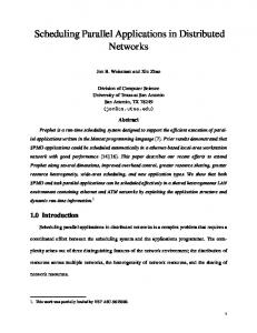
Fig. 1: A simple split-join graph and a task graph derived from it. Actor B has α instances. model of bounded-resource DMA communication and the corresponding method to let the SMT solver to jointly orchestrate parallel computations and multi-channel DMA transfers. The computed schedules for tasks and DMA transfers, are deployed using a run-time to execute real applications on a many-core platform with over 250 cores and 16 clusters. The paper is organized as follows. In Sec. II we introduce the basic notions of the split-join and task graph. In Sec. III we introduce the many-core platform and the proposed intertask communication scheme for split-join-graphs. Next, in Sec. IV we describe the design flow. In Sec. V we present the methodology to model the communication with bounded communication memory and network flow control. In the following section we present a model that represents joint scheduling of computation and communication (DMA) tasks. Then we show how that model is presented to an SMT solver in the form of constraints. Sec. VII presents the experiments with a set of application benchmarks. Sec. VIII concludes the paper and discusses the related and future work. II. S PLIT-J OIN G RAPHS Definition 1 (Split-Join and Task Graphs): A split-join graph S is a tuple S = (V, E, d, α, ω) where (V, E) is a directed acyclic graph (DAG), that is, a set V of actors, a set E ⊆ V × V of edges with no cyclic paths. The function d : V → R+ defines the node delay, α : E → Q+ assigns a parallelization factor to every edge. An edge e can be either a split, join or neutral, depending on whether α(e) = a, 1/a or = 1 for some integer a > 1, which counts the tasks at data split and join. ω(e) denotes the size of data tokens sent to each spawned task in the case of split, or received from each joined task in the case of join, or just sent and received if the edge is neutral. A split-join graph with α(e) = 1 for every e is called a task graph and is denoted by T = (U, E, δ, ω), where the four elements in the tuple correspond to V , E, d, and ω.

The split-join graph is a generalization of the task graph by data parallelism, explicitly represented by parallelization factors α. This is illustrated by the example in Fig. 1. A label α on the edge from A to B means that every executed instance of task A spawns α instances of task B. Likewise, a 1/α label on the edge from B to C means that all those instances of B should terminate and their outputs be joined before executing C (see Fig. 1). A task graph can thus be viewed as derived from the split-join graph by making data parallelism explicit. We call the nodes of the split-join graphs actors and those of the task graph tasks. The edges of a split-join graph e ∈ E are called channels, and those in a task graph  ∈ E are called dependency arcs or just dependencies. We use the graph-theoretic models not only to model the tasks and dependencies of the application, but also those of the implementation. For this purpose, it is convenient to generalize the split-join graph model into a semantically richer model. Definition 2 (Marked graph): The marked (split-join) graph S can be defined as a split-join graph extended by allowing cyclic paths and introducing an extra edge parameter – the marking: m : E → N≥0 . We assume that any split-join graph is a marked graph with zero marking.

A. The Semantics of Split-join and Marked Graphs In split-join graphs, the tasks (i.e., instances of an actor) can execute in parallel unless there are dependencies between them. In Fig. 1 actor A spawns α instances of actor B which can execute in parallel. Still, for convenience, we explain the functional behavior from sequential-execution point of view. In sequential execution, a channel e = (v, v 0 ) can be seen as a FIFO (first-in-first-out) buffer. The task instances of each actor v execute in a fixed order, which determines their index: v0 , v1 , v2 etc.. The instances vq of the writer actor of channel (v, v 0 ) produce α↑ (v, v 0 ) tokens each in the FIFO channel; in the derived task graph α↑ also corresponds to the number of outgoing dependency arcs of vq . Similarly, α↓ (v, v 0 ) denotes the number of tokens consumed and the number of incoming arcs of the channel reader actor instances vr0 . We have: ( ( α(e) α(e) ≥ 1 1 α(e) ≥ 1 ↑ ↓ α (e) = ; α (e) = −1 1 α(e) < 1 α(e) α(e) < 1 The tokens have size ω bytes, and the amount of data produced by an instance of v and consumed by an instance of v 0 is: w↑ (e) = α↑ (e) · ω(e); w↓ (e) = α↓ (e) · ω(e) Thus defined, the split-join graph can be viewed as a special case of SDF (synchronous dataflow) graphs [4], which consist of actors that write and read a fixed amount of data to FIFO channels. An important property of an SDF graph is its consistency [4], which requires that there must exist a positive integer function c : V → N+ such that after executing c(v) instances of all actors we have that at each channel the number of tokens produced is equal to the number of tokens consumed. The equations that express the consistency requirement are

known as balance equations: ^ α↑ (v, v 0 ) · c(v) = α↓ (v, v 0 ) · c(v 0 )

(1)

(v,v 0 )∈E

Note that if Eq. (1) has a solution c(v) then k·c(v), ∀k ∈ N+ is a solution as well. However, we consider only the minimal positive integer solution and use the notation c(v) for it. Executing each actor c(v) number of times is defined as SDF graph iteration. B. Derived Task Graph The task graph derived from a split-join graph models one graph iteration.1 For each actor v the task graph contains c(v) tasks {v0 , v1 , . . . vc(v)−1 }, i.e., the instances of actor v. Let us define the edges of the derived task graph. For a split-join channel (v, v 0 ) with α(v, v 0 ) = a/b let us consider the sequence of a · c(v) tokens produced in the FIFO buffer in one iteration. Let us number these tokens by index i in the order they are produced by the instances of actor v : v0 , v1 , . . . . Obviously, token i is produced by task vq where q = bi/ac. In sequential execution the actor instances consume tokens in the same order as they are produced (the FIFO order). Therefore, the first b tokens will be consumed by task v00 , then the next b tokens by v10 , etc. In general, token i is consumed by task vr0 where r = bi/bc. To model this producer-consumer dependency, the task graph should contain edge (vq , vr0 ). A non-zero marking m0 = m(v, v 0 ) has the semantics of initial availability of m0 tokens in the channel. Therefore, for the case of a marked graph in the above example we have to calculate r as r = b(i + m0 )/bc. Definition 3 (Derived Task Graph): From a consistent marked split-join graph S = (V, E, d, α, ω, m) we derive the task graph T = (U, E, δ, ω) as follows: U = {vh | v ∈ V, 0 ≤ h < c(v)} E = {(vh , vh0 0 ) | (v, v 0 ) ∈ E ∧ (v, v 0 , h, h0 )} where  is a predicate defined by: (v, v 0 , h, h0 ) : ∃ i ∈ N : h = bi/α↑ (v, v 0 )c, h0 = b(i + m(v, v 0 ))/α↓ (v, v 0 )c, vh , vh0 ∈ U We also define that: ∀(vh , vh0 0 ) ∈ E ω(vh , vh0 0 ) = ω(v, v 0 ), ∀vh ∈ U δ(vh ) = d(v) We use derived task graphs to define the scheduling constraints in Sec. VI. III. T HE M ANY- CORE P LATFORM A. Many-core Hardware Architecture Many-core processors can be seen as a hybrid of two simpler on-chip multiprocessor types. Those are multi-cores (shared-memory on-chip multiprocessors) and multiprocessor networks-on-chip. In many-cores, multiple multi-core clusters are networked on a chip. One of important usage scenarios is 1 In SDF terminology, deriving a task graph is equivalent to deriving a homogeneous SDF graph.

where a host CPU runs the usual software stack and generalpurpose tasks, whereas computationally expensive highly parallel kernels are forwarded to a many-core chip. MPPA [5] of Kalray, P2012 [6] of ST Micro, and SCC of Intel [7] are a few examples of many-core platforms. In our experiments, we use Kalray MPPA. This platform contains 256 symmetrical cores. The cores are grouped in 16 compute clusters of 16 cores each. The clusters are connected by a network-on-chip (NoC) with a toroidal 2D topology. Each cluster has 2MB of shared scratchpad memory. The cores have caches to access this memory, however, in our current work we disable them. A cluster also has a DMA control unit with 8 DMA channels. They are used for explicit data transfers to other clusters through the NoC. For efficiency, we use asynchronous transfers, i.e., those that return the control back to the compute core before the transfer is completed. We characterize the delay T (s) of a data transfer as per [8] as follows: T (s) = I + g · s

(2)

where I is the fixed initialization delay, s is the size of transfer in bytes, and g is the delay per byte, which depends on the throughput of the network communication links. It is important to note that during the time I both the compute core and the DMA channel are busy for setting up the transfer, whereas during the remaining time G = g · s only the DMA channel is still busy, pushing the data into the NoC, while the core can proceed to other tasks in parallel. DMA transfer completion status can be polled from any core inside the cluster. This operation is blocking until time T (s) has elapsed plus some additional timing delay χ to return the control back to the thread waiting for transfer completion. Definition 4 (Architecture Model): An architecture model A is a tuple (X, H, M , D, I, g, χ), where X is a set of clusters, H ⊆ X ×X is a set of communication paths between pairs of clusters, whereas |(x, x0 )|H gives the topological distance between any two clusters. M and D are the number of cores and DMA channels per cluster respectively. I, g, χ ∈ R+ are communication delay components introduced earlier. B. Support of Communication Buffers In the split-join graph application model, the actors communicate via channels. Given the limits of memory size of the platform, the channels should use a bounded memory. Moreover, to exploit the data parallelism of the split-join channels, it should be possible to execute different concurrent instances of channel writer and reader on different cores. We created a software buffer implementation that satisfies these requirements. To support concurrent writers and readers we exploit the fact that in a split-join graph each writer/reader instance writes/reads statically known amounts of data at statically known offsets. Therefore, each data token place in the buffer is equipped by an individual status record, which can be updated independently and which indicates whether the given token is ready to be written or read. For a buffer of limited size we use standard circular-buffer wrap-around mechanism, with a wrap-around counter in each status record.

The communication protocol is more complex when the writer and reader actors are located in different clusters. In this case we split the FIFO buffer into writer and reader sub-buffers, the latter being located in the remote cluster. The data is copied from the writer sub-buffer to the reader by a DMA transfer. Along with this data transfer, also the ‘writing finished’ status record update is sent for the reader sub-buffer. For its part, the reader sends the ‘reading finished’ status update for the same sub-buffer back to the writer. This allows the writer, prior to transferring another data token through DMA, to safely estimate whether a remote buffer place is ready for this token. This backward signalling of buffer space availability is usually referred to as flow control. More details about DMA communication become apparent in later sections. IV. D ESIGN F LOW Given a many-core architecture, the problem is to map and schedule an application model, represented by a split-join graph called application graph and denoted S M =(V M ,E M ,d,α,ω). The design flow is based on multi-criteria optimization, whereby we repeatedly query the SMT solver for solving the problem at different points in the multi-dimensional cost space, to approximate the Pareto front in a manner of a ‘multidimensional binary search’, as proposed in [3]. In general, combined scheduling, mapping and buffer allocation inside a shared-memory cluster is hard if one tries to solve it exactly using the SMT solvers, but one can still approximate the optimal solutions and bound the approximation distance, see e.g., [2], [3]. To tackle the problem complexity, we solve it in three steps: (i) partitioning, (ii) placement, and (iii) scheduling. Thus the solutions found are optimal only locally, in the context of each step. Nevertheless, in the third step we combine several communication and computation decisions together to have a jointly optimal result. In this section we briefly sketch the design flow as a whole, whereas in the rest of the paper we focus on the methodology of the scheduling step, the core contribution of this paper. The partitioning step defines the groups of actors to be assigned to the same many-core cluster. We adapt the partitioning scheme of [3] to the split-join graph model. Partitioning Problem Instance: Application graph S M =(V M ,E M ,d,α,ω) and the costs: - Cτ : Maximum computation workload per partition - Cη : Estimated total communication cost - Cz : Number of partitions The computation and communication workload are calculated as the sum of task execution delays or data token sizes in the derived task graph respectively. A channel contributes to the communication cost only if the channel writer and reader are assigned to different partitions. Partitioning Problem Solution z : V M → N≥0 where z(v) identifies the partition of actor v. The approximate Pareto points in three-dimensional cost space obtained at the this step are propagated to placement and

eˆ : [α(ˆ e), ω(ˆ e)]

e : [α(e), ω(e)] A

B

Fig. 2: Communicating Tasks Gwr

ert (ˆ e) : [α(ˆ e), ω(ˆ e)]

Fig. 4: Buffer aware graph model for a channel without DMA B

Fig. 3: Partition Aware Communicating Tasks scheduling steps. The latter two are considered independent, as we currently ignore the network routing and contentions. The placement step allocates a unique physical cluster to every partition. The purpose is to map the pairs of communicating partitions to clusters x, x0 located as close as possible, to minimize the total communication cost according to metric s · |x, x0 |H , where s is the communication data size. The SMT solver constraints at this step are again similar to those in [3]. In the scheduling step we perform a joint scheduling of the computation tasks (i.e., the tasks of the application graph) and the communication tasks (i.e., the DMA transfers). In this paper we first describe a model that captures the interactions between computation and communication tasks. Then we explain how this model is encoded in terms of SMT solver constraints. The model is derived from a series of graph transformations, which gradually change the application graph into a final schedule graph. V. M ODELING C OMMUNICATION A. Partition Aware Graph For defining the graph transformations, in particular for adding new actors, it is convenient to introduce notation v : [d(v), z(v)], which represents an actor v with delay d(v) and partition number z(v). Similarly, e : [α(e), ω(e), m(e)] represents an edge e with parallelization factor α(e), token size ω(e) and marking m(e). The latter two parameters are sometimes omitted, the default values being zero. Note that if ω is zero, the given edge models an execution order constraint and does not involve a memory buffer for communication. We assume to have a ready partitioning solution z(v), calculated earlier in the design flow. In order to model the communication delay, we need to introduce additional actors in the split-join graph, representing the DMA transfers. Recall from Equality (2) that a DMA transfer consists of two phases: the initialization, modeled here by actor Iwr , and the network communication, modeled by actor Gwr . Fig. 2 shows an application graph channel eˆ = (A, B) and Fig. 3 shows its partition aware graph for the case where actors A and B are assigned to different partitions. Recall that in this case the channel (A, B) is split into writer and reader sub-buffers. Edge ewt (ˆ e) models the writer sub-buffer; α = 1 indicating that one writer instance is followed by exactly one data transfer, whereas ω(ewt ) = w↑ indicates that all α↑ tokens produced by an instance of the writer actor are encapsulated into a compound token. Edge ewn (ˆ e) reflects the sequential order between the two DMA phases. Edge ert (ˆ e) corresponds to the reader sub-buffer. It has the same parameters as the original edge eˆ.

ewt : [1, w↑ ]

A ew

b

:[ 1,

Iwr

ewn : [1] Gwr er b : [α − 1 ,0 , b( er

ert : [α, ω]

1]

ewn (ˆ e) : [1]

0,

:[

Iwr

b(

s

ewt (ˆ e) : [1, w↑ (ˆ e)]

ebe (e) : [α−1 (e), 0, b(e)]

ew

ew

A

B

t )]

t)

]

Fst

B ers : [1]

A

Grd

ern : [1]

Ird

Fig. 5: Buffer aware graph model for a channel with DMA M Let E∆Z denote the channels crossing the partition boundM aries and E∆Z its complement. Formally, M E∆Z = {(v, v 0 ) ∈ E M | z(v) 6= z(v 0 )} M M = E M \ E∆Z E∆Z Definition 5 (Partition Aware Graph): A partition aware graph S P = (V P , E P , d, α, ω) is a split-join graph obtained M by replacement of application graph edges E∆Z by a subgraph with new actors and edges as defined below. The delay of the new actors is determined by the DMA initialization time I and the network sending time g · w↑ (ˆ e). P M V = V ∪ {Iwr (ˆ e) : [I, z(v)], M Gwr (ˆ e) : [g · w↑ (ˆ e), z(v)] | eˆ = (v, v 0 ) ∈ E∆Z } The edges of partition aware graph are given by: M M E P = E∆Z ∪ {ewt (ˆ e), ewn (ˆ e), ert (ˆ e) | eˆ = (v, v 0 ) ∈ E∆Z } Edge & Parameters ewt (ˆ e) : [1, w↑ (ˆ e)] ewn (ˆ e) : [1] ert (ˆ e) : [α(ˆ e), ω(ˆ e)]

Connections ewt (ˆ e) = (v, Iwr (ˆ e)) ewn (ˆ e) = (Iwr (ˆ e), Gwr (ˆ e)) ert (ˆ e) = (Gwr (ˆ e), v 0 )

B. Buffer Aware Graph After we obtain a partition aware graph, the next graph transformation is performed in order to model the bounded buffer memory allocated to the channels. Definition 6 (Buffer Allocation): b : E P → N+ defines the bounded capacity assigned the channels of the partition-aware graph. It is part of the solution of the combined multiprocessor scheduling and buffer allocation problem. Definition 7 (Buffer Aware Graph): is a cyclic marked graph S B = (V B , E B , d, α, ω, m) obtained from the partitionaware graph by adding marked channels that model the allocated buffer capacity and new actors that model the DMA polling and flow control. In this graph, for each intra-cluster channel eˆ we add a new backward channel – in the opposite direction, marked with the buffer allocation b(ˆ e), modeling the ‘communication’ of the available space in the channel. The backward channel is the inversion of eˆ, with inversely proportional parallelization factor, see Fig. 4. Recall that the marking models the number of tokens present in the channel at the start of the execution. In the backward

channel the marking b(ˆ e) indicates the free space that is available initially. At every execution, the writer takes α↑ tokens of ‘space’ and produces α↑ tokens of data, and the reader takes α↓ tokens of data and produces α↓ tokens of ‘space’.2 If the channel is an inter-cluster channel, involving DMA, then we model the bounded space of the writer sub-buffer, ewt , and the reader sub-buffer, ert , by separate backward channels. We also add additional actors, see Fig. 5. Consider the writer sub-buffer, ewt , serving as an input to the DMA transfer. The space in this sub-buffer becomes available when the transfer is completed. Recall that detecting the transfer completion costs processor time, this is modelled by new actor Fst . This actor produces the ‘space’ tokens on the backward channel of ewt . Recall that for flow control the free space availability status of the reader sub-buffer, ert , has to be communicated back to the writer. The respective DMA transfer is modeled by Ird and Grd , and the latter feeds the ‘space’ tokens to the backward channel of ert . Consider an example. Suppose that we use a doublebuffering approach, such that b(ewt (A, B)) = b(ert (A, B)) = 2 tokens. Let us simulate the execution of the model in Fig. 5 unfolded for three actor instances: A0 , A1 , A2 – see Fig. 6. • A0 executes and consumes one space token. • Upon completion, A0 triggers a DMA transfer initialization, modeled by Iwr0 • Data is sent to the network, which is represented by Gwr0 . In parallel, A1 picks the second space token and triggers another DMA transfer: Iwr1 and Gwr1 . • When Gwr0 finishes, B0 receives the input data tokens. At the end it releases the space occupied by these tokens and triggers a DMA transfer to update the writer accordingly. This transfer is modeled by Ird0 and Grd0 . • A2 waits execution for task Fst0 to finish, which releases the necessary space token in the backward channel. • After A2 , we can start transferring its output by Iwr2 when we receive the (flow-control) space token via Grd0 Below we formalize the new actors and channels: V B = V P ∪ {Fst (ˆ e) : [χ, z(v)], Ird (ˆ e) : [I, z(v 0 )], ↓

0

0

M E∆Z }

Grd (ˆ e) : [α (ˆ e) · ω0 · g, z(v )] | eˆ = (v, v ) ∈ The delay of network sending node α↓ · ω0 · g corresponds to the delay of sending ω0 bytes of status record for all α↓ tokens read in the channel, where ω0 depends on the implementation. E B = E P ∪ {ews (ˆ e), ewb (ˆ e), ers (ˆ e), M ern (ˆ e), erb (ˆ e) | eˆ = (v, v 0 ) ∈ E∆Z }∪ M } {ebe (ˆ e) : [α−1 (ˆ e), 0, b(ˆ e)] | eˆ = (v, v 0 ) ∈ E∆Z

Edge & Parameters ews (ˆ e) : [1] ewb (ˆ e) : [1, 0, b(ewt (ˆ e))] ers (ˆ e) : [1] ern (ˆ e) : [1] erb (ˆ e) : [α-1 (ˆ e), 0, b(ert (ˆ e))]

Connections ews (ˆ e) = (Iwr (ˆ e), Fst (ˆ e)) ewb (ˆ e) = (Fst (ˆ e), v) ers (ˆ e) = (v 0 , Ird (ˆ e)) ern (ˆ e) = (Ird (ˆ e), Grd (ˆ e)) erb (ˆ e) = (Grd (ˆ e), Iwr (ˆ e))

2 Note that if we derive a task graph from a buffer aware graph then its structure will depend on the buffer sizes such that a smaller buffer size can only increase the critical path delay (a buffer-latency trade-off).

precedence dependency

Dma2

blocked

P roc2 Dma1 P roc1

Ird0

backward dependency (space)

Iwr0 A0

Grd0

B0 Gwr0

Iwr1

A1

Gwr1 Fst0

Iwr2 A2

Time

Fig. 6: Double buffering schedule example C. Communication Aware Graph In our implementation the compute core remains busy until the completion of the DMA initialization tasks (Iwr or Ird ) that follow after the corresponding computation actor (writer or reader, resp.). Moreover, if the computation actor instance starts multiple DMA transfers (as a writer/reader of multiple channels), then the next DMA transfer cannot start until the initialization of the previous transfer has finished. This restriction can be modeled by adding extra edges between the actors modeling the DMA initialization phase, to enforce a sequential execution order in the schedule. Definition 8 (Communication Aware Graph): Communication Aware Graph S K = (V K , E K , d, α, ω, m) is obtained from the buffer aware graph S B by adding the edges to model the ordering of the DMA transfers with regard of their transfer initialization phase. The set of actors of the communication aware graph is the same as in the buffer aware graph V K = V B . To define the new edges, we first introduce function I(v), representing an ordered set of the transfer initialization actors connected to the output of given actor v, i.e., I(v) = {v 0 | (v, v 0 ) ∈ E B ∧ ∃ eˆ ∈ E M : v 0 = Iwr (ˆ e) ∨ v 0 = Ird (ˆ e)} We select the order (I1 , I2 , . . . | Ik ∈ I(v)) arbitrarily, ensuring that the implementation and the model follow the same order. We have: E K = E B ∪ {(Ii , Ii+1 ) : [1] | Ii , Ii+1 ∈ I(v), v ∈ V B } The final transformation to model the communication is the derivation of the task graph T K = (U K , E K , δ, ω) from the split-join graph S K . This is done according to Def. 3, but in addition we require that the tasks inherit the partitioning from their actors: ∀vh ∈ U K z(vh ) = z(v). Having shown our model for buffered DMA communication, we proceed to the scheduling model in the next section. VI. S CHEDULING A. Schedule Graph The schedule graph T S = (U S , E S , δ, ω) is obtained from computation aware task graph T K by adding the mutual exclusion edges, according to the given schedule s and intracluster mapping µ, where: - µ : U S → N≥0 maps every task to a core (for computation tasks) or a DMA channel (for transfer tasks);

s : U S → R≥0 associates each task with a start time. The buffer allocation, b, the schedule and the mapping should be calculated by the solver in the scheduling step of the design flow, as explained later. Let us recall and introduce some notations. S S S •- U = UT ∪ UC is the task partitioning into: – transfer tasks UTS , derived from DMA transfer actors: Iwr , Gwr Ird , and Grd . – computation tasks UCS • I(u) are the transfer tasks connected to the output of task u, by analogy to I(v) of the computation-aware graph. S • UC+ is the set of computation tasks connected to DMA S transfers: UC+ = {u ∈ UCS | I(u) 6= ∅} S • UC∅ is the set of the remaining computation tasks, i.e., those with no DMA transfer tasks at the output. Note that not all tasks introduced for communication are transfer tasks. In fact, Fst (see Fig. 5) are computation tasks, as they are executed on the compute cores. Due to a limited number of the compute cores and DMA channels multiple tasks are mapped to the same core or channel, and should therefore be executed sequentially. This requirement is modeled by adding mutual exclusion edges. The edges of the schedule graph are therefore defined by: µ µ E S = E K ∪ ETµ ∪ EC∅ ∪ EC+ are the mutual exclusion edges for the transfer tasks mapped at the same DMA channel. ETµ = {(u, u0 ) : [1] | u, u0 ∈ UTS ,

ETµ

z(u) = z(u0 ), µ(u) = µ(u0 ), s(u0 ) ≥ s(u)} Similarly, we insert an edge for the computation tasks mapped on the same core, first for the case of no DMA transfers: µ S EC∅ = {(u, u0 ) : [1] | u ∈ UC∅ , u0 ∈ UCS 0

0

0

z(u) = z(u ), µ(u) = µ(u ), s(u ) ≥ s(u)} Finally, given task u that starts some DMA transfers, let Imax (u) represent the last transfer in the ordered set (I1 (u), I2 (u), . . . ). The compute core becomes available to a later task u0 only when the last transfer initialization is completed: µ S EC+ = {(Imax (u), u0 ) : [1] | u ∈ UC+ , u0 ∈ UCS , z(u) = z(u0 ), µ(u) = µ(u0 ), s(u0 ) ≥ s(u)} B. Scheduling Problem on SMT solver In the previous sections we described a sequence of rules to derive a schedule graph, which models the timing effect of a scheduling/buffering solution calculated by the SMT solver. The solver constraints for this problem are therefore obtained directly from the schedule graph. Below we present the corresponding definition of the optimization problem dealt with at the scheduling step of the design flow. Problem Instance: P • partition-aware graph S • hardware architecture model A, • costs for multi-criteria optimization: – CB : maximal buffer memory size per cluster – CL : schedule latency constraint

Solution: (T S , b, µ, s), where T S = (U S , E S , δ, ω) is the schedule graph obtained from S P by adding extra edges based on buffering b, mapping µ and scheduling s. Schedule constraints The schedule should respect all the dependencies, including the application dependencies, bounded buffer space, DMA transfer ordering, and mutual exclusion, all represented by dependency arcs in the schedule graph: ^ s(u0 ) ≥ s(u) + δ(u) (u,u0 )∈

E S (b,s,µ)

As we explicitly indicate here, the set of schedule dependencies is function of the problem solution. However, the SMT solvers require a static set of constraints. Therefore, observing that the set U S is static we rewrite the constraints as: ^ S (u, u0 , µ, s, b) =⇒ s(u0 ) ≥ s(u) + δ(u) u,u0 ∈U S S

where  is a predicate asserting the presence of dependency arc (u, u0 ). For mutual exclusion arcs this predicate can be trivially obtained from the definition of sets E µ . For backward edges it can be obtained from (v, v 0 , h, h0 ) in Def. 3, by substituting the buffer allocation to marking m. However, we did not yet implement in the SMT constraints for the backward edges, therefore we replaced them by equivalent constraints proposed in [2], slightly adapted to the channels with DMA. Resource constraints Bounded number of DMA channels and cores per cluster. ^ ^ µ(u) < |D| ∧ µ(u) < |M | u∈UTS

S u∈UC

Bounded buffer memory per cluster: ^ X b(e) · ω(e) ≤ CB z 0 ∈Z

e=(v,v 0 )∈E P :z(v 0 )=z 0

Latency constraint ^

s(u) + δ(u) ≤ CL

u∈U S

Extra constraints In our implementation we require the writer and reader subbuffers to have equal buffer memory: ^ b(ewt (ˆ e)) · ω(ewt (ˆ e)) = b(ert (ˆ e)) · ω(ert (ˆ e)) M eˆ∈E∆Z

The network phase of a DMA transfer should run immediately after the initialization phase on the same channel: ^ ^ s(Iwr h (ˆ e)) + I = s(Gwr h (ˆ e)) ∧ M 0≤h