Multiprocessor Scheduling of Precedence-constrained ... - Verimag

Multiprocessor Scheduling of Precedence-constrained Mixed-Critical Jobs Dario Socci, Peter Poplavko, Saddek Bensalem, Marius Bozga Verimag Research Report no TR-2014-11 November 2014

Reports are downloadable at the following address http://www-verimag.imag.fr

Unite´ Mixte de Recherche 5104 CNRS - Grenoble INP - UJF Centre Equation 2, avenue de VIGNATE F-38610 GIERES tel : +33 456 52 03 40 fax : +33 456 52 03 50 http://www-verimag.imag.fr

Multiprocessor Scheduling of Precedence-constrained Mixed-Critical Jobs Dario Socci, Peter Poplavko, Saddek Bensalem, Marius Bozga

November 2014

Abstract The real-time system design targeting multiprocessor platforms leads to two important complications in real-time scheduling. First, to ensure deterministic processing by communicating tasks the scheduling has to consider precedence constraints. The second complication factor is mixed criticality, i.e., integration upon a single platform of various subsystems where some are safety-critical (e.g., car braking system) and the others are not (e.g., car digital radio). Therefore we motivate and study the multiprocessor scheduling problem of a finite set of precedence-related mixed criticality jobs. This problem, to our knowledge, has never been studied if not under very specific assumptions. The main contribution of our work is an algorithm that, given a global fixed-priority assignment for jobs, can modify it in order to improve its schedulability for mixed-criticality setting. Our experiments show an increase of schedulable instances up to a maximum of 30% if compared to classical solutions for this category of scheduling problems. Keywords: real-time, mixed critical, scheduling, multiprocessor Reviewers: How to cite this report: @techreport {TR-2014-11, title = {Multiprocessor Scheduling of Precedence-constrained Mixed-Critical Jobs}, author = {Dario Socci, Peter Poplavko, Saddek Bensalem, Marius Bozga}, institution = {{Verimag} Research Report}, number = {TR-2014-11}, year = {2014} }

Dario Socci, Peter Poplavko, Saddek Bensalem, Marius Bozga

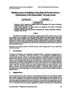
Figure 1: Proposed algortirhm MCPI. T stands for task graph and P T for priority table.

1

Introduction

The real-time system design targeting multi and many-core platforms leads to two important issues. Firstly, to ensure deterministic processing by communicating tasks one has to consider scheduling problems with precedence constraints, i.e., task graphs. Such tasks often have multiple execution rates and hence their jobs have different arrival times and deadlines [1]. However, the precedence constrained scheduling theory for multiple processors usually considers common arrival times and deadlines of connected jobs. Luckily many practical applications are not sporadic but synchronous-periodic, so they can be modeled by a finite task graph that represents one hyperperiod and enables simple static analysis. We abstract from job periodicity and consider just a static set of jobs with arbitrary statically known arrival times, deadlines, and precedence relations. Modern technology opens the possibility to integrate upon a single chip various subsystems which required multiple chips and boards in the past, which offers power and weight savings. However, this integration leads to the second issue we raise here – the mixed criticality. The point is that some subsystems are safety critical [2]; therefore, according to current industry standards, one cannot let other subsystems share resources with them, to avoid that their errors and faults have consequences for the safety critical subsystems. The current industry practice assumes complete time or space isolation of subsystems having different levels of criticality, which reduces the benefits of integration. It is much more efficient [3] to let the scheduler use the resources in a flexible way during the normal operation, and only when faults occur give all the resources entirely to the safety critical subsystems, to provide them ample means for fault recovery. In addition, one needs to protect highly critical subsystems from timing misbehavior, especially execution time overruns of less critical ones [4]. For static sets of jobs on single processor, the basic principles and results of corresponding scheduling policies were presented in [3], whereas we investigate extensions towards precedence constraints and multiple processors. For mixed criticality scheduling problems Audsley approach can be used for correct priority assignment [1], but this approach is mainly restricted to uniprocessor scheduling [5]. This is because Audsley approach is based on the assumption that the completion time of the job with the least priority may be computed ignoring the relative priority of the other jobs. This assumption is no longer true in multiprocessors systems. Audsley approach can still be used, by using pessimistic formulas to compute the completion time of the least priority job [5]. However, in the case of finite set of jobs, it can be hard to find a formula with an acceptable level of pessimism. The main contribution of this paper is the Mixed Criticality Priority Improvement (MCPI ) algorithm, that overcomes the limitation of Audsley approach in multiprocessor system. MCPI, in fact, assigns priorities starting from the highest. This allows us to compute exact completion times. The drawback of this approach is that, unlike Audsley approach, just picking up a job that meets the deadline is not enough for correctness. For this reasons we need an heuristic to help us to select a “good” job in each step. Fig. 1 shows an overview of MCPI. The algorithm takes as input the task graph T, the number of processors m and a priority table PT. The latter may be generated by any known multiprocessor algorithm. We call this algorithm support algorithm. The algorithm is based on the concept of Priority Direct Acyclic Graph (P-DAG), which defines a partial order on the jobs showing sufficient priority constraints needed to obtain a certain schedule. We build such a structure by adding, at each step, jobs from PT, starting from the one with the highest priority. Each time we add a job, we apply a modification to the priority order given by table PT, to increase the schedulability of safety critical scenarios. When

Verimag Research Report no TR-2014-11

1/27

Dario Socci, Peter Poplavko, Saddek Bensalem, Marius Bozga

the construction of the P-DAG is terminated, we generate a new priority table by topological sort of the P-DAG. The paper is organized as follows. Section 2.1 gives an introduction to the formalism of multiprocessor scheduling in Mixed Critical System. Section 3 defines P-DAGs and their properties. The MCPI algorithm is then described in Section 4. In Section 5 we discuss the related work and in Section 6 we give experimental results. Finally in Section 7 we discuss conclusions and future work.

2

Scheduling Problem

2.1

Problem Definition

In a dual-criticality Mixed-Critical System (MCS), a job Jj is characterized by a 5-tuple Jj = (j, Aj , Dj , χj , Cj ), where: • j ∈ N+ is a unique index • Aj ∈ Q is the arrival time, Aj ≥ 0 • Dj ∈ Q is the deadline, Dj ≥ Aj • χj ∈ {LO, HI} is the job’s criticality level • Cj ∈ Q2+ is a vector (Cj (LO), Cj (HI)) where Cj (χ) is the WCET at criticality level χ. We assume that Cj (LO) ≤ Cj (HI)[3]. We also assume that the LO jobs are forced to complete after Cj (LO) time units of execution, so (χj = LO) ⇒ Cj (LO) = Cj (HI). A task graph T of the MCscheduling problem is the pair (J, →) of a set J of K jobs with indexes 1 . . . K and a functional precedence relation →⊂ J × J. The criticality of a precedence constraint Ja → Jb is HI if χ(a) = χ(b) = HI. It is LO otherwise. A scenario of a task graph T = (J, →) is a vector of execution times of all jobs: (c1 , c2 , . . . , cK ). If at least one cj exceeds Cj (HI), the scenario is called erroneous. The criticality of scenario (c1 , c2 , . . . , cK ) is the least critical χ such that cj ≤ Cj (χ), ∀j ∈ [1, K]. A scenario is basic if for each j = 1, . . . , K either cj = Cj (LO) or cj = Cj (HI). A (preemptive) schedule S of a given scenario is a mapping from physical time to J × J × . . . × J = Jm  where J = J ∪ {}, where  denotes no job and m the number of processors available. Every job should start at time Aj or later and run for no more than cj time units. A job may be assigned to only one processor at time t, but we assume that job migration is possible to any processor at any time. Also for each precedence constraint Ja → Jb , job Jb may not run until Ja completes. A job J is said to be ready at time t iff: 1. all its predecessors completed execution before t 2. it is already arrived at time t 3. it is not yet completed at time t The online state of a run-time scheduler at every time instance consists of the set of completed jobs, the set of ready jobs, the progress of ready jobs, i.e., for how much each of them has executed so far, and the current criticality mode, χmode , initialized as χmode = LO and switched to ‘HI’ as soon as a HI job exceeds Cj (LO). A schedule is feasible if the following conditions are met: Condition 1. If all jobs run at most for their LO WCET, then both critical (HI) and non-critical (LO) jobs must complete before their deadline, respecting all precedence constraints. Condition 2. If at least one job runs for more then its LO WCET, than all critical (HI) jobs must complete before their deadline, whereas non-critical (LO) jobs may be even dropped. Also LO precedence constraints may be ignored.

2/27

Verimag Research Report no TR-2014-11

Dario Socci, Peter Poplavko, Saddek Bensalem, Marius Bozga

Figure 2: The graph of an airplane localization system illustrating LO→HI dependencies.

The reason why we allow to have precedences from LO jobs to HI jobs can be seen in the example of Fig. 2. There we have a task graph of the localization system of an airplane, composed of four sensors (jobs s1-s4) and the job L, that computes the position. Data coming from sensor s4 is necessary and sufficient to compute the plane position with a safe precision, thus only s4 and L are marked as HI critical. On the other hand, data from s1, s2 and s3 may improve the precision of the computed position, thus granting the possibility of saving fuel by a better computation of the plane’s route. So we do want job L to wait for all the sensors during normal execution, but when the systems switch to HI mode we only wait for data coming from s4. Based on the online state, a scheduling policy deterministically decides which ready jobs are scheduled at every time instant on m processors. A scheduling policy is correct for the given task graph T if for each non-erroneous scenario it generates a feasible schedule. A scheduling policy is predictable, if an earlier completion of a job may not delay the completion of another job. A task graph T is MC-schedulable if there exists a correct scheduling policy for it. A fixed-priority scheduling policy is a policy that can be defined by a priority table P T , which is a vector specifying all jobs in a certain order. The position of a job in P T is its priority, the earlier a job is to occur in P T the higher the priority it has. Among all ready jobs, the fixed-priority scheduling policy always selects the m highest-priority jobs in P T . A priority table P T defines a total ordering relationship between the jobs. If job J1 has higher priority than job J2 in table P T , we write J1 P T J2 or simply J1  J2 , if P T is clear from the context. In this paper we assume global fixed-priority scheduling which allows unrestricted job migration. A priority table P T is required to be precedence compliant i.e., the following property should hold: J → J 0 ⇒ J P T J 0

(1)

The above requirement is reasonable, since we may not schedule a job before its predecessors complete. The use of fixed-priority in combination with the adopted precedence aware definition of ready job is called in literature List Scheduling. We combine list scheduling with fixed priority per mode (FPM), a policy with two tables: P TLO and P THI . The former includes all jobs. The latter only HI jobs. As long as the current mode is LO, this policy performs the fixed priority scheduling according to P TLO . After a switch to the HI mode, this policy drops all pending LO jobs and applies priority table P THI . Since scheduling after the mode switch is a singlecriticality problem, such a table can be obtained by using classical approaches. Therefore, we focus on producing the table P TLO , in the following simply denoted as P T . Fixed-priority (FP) policy (without precedences), is predictable [6], while list scheduling (with precedences) is not, therefore, for the online scheduling we modify this policy to ensure predictability as described in Sec. 4.2. For predictable policies it is sufficient to restrict the offline schedulability check to simulation of basic scenarios [3]. To be more specific [7], firstly, we check the scenario with execution times cj = Cj (LO), i.e., the LO scenario. Secondly, for each HI job Jh , we check the scenario where the jobs that completed before Jh have cj = Cj (LO), while the other jobs (including Jh ) have cj = Cj (HI). Such a scenario is denoted HI[Jh ]. We check these scenarios offline under list scheduling, and then use their start times as arrival times online.

Verimag Research Report no TR-2014-11

3/27

Dario Socci, Peter Poplavko, Saddek Bensalem, Marius Bozga

2.2

Characterization of Problem Instance

To characterize the performance of scheduling algorithms one uses the utilization and the related demandcapacity ratio metrics. For a job set J = {Ji } and an assignment of execution times ci the appropriate metric is load [8]: P Ji ∈J: t1 ≤Ai ∧Di ≤t2 ci `oad (J, c) = max 0≤t1 th the highest priority, for a certain threshold th. Ties are broken arbitrarily. For the other jobs, the priority is the default EDF. Obviously, this strategy resolves the Dhall-effect counterexample mentioned earlier. However this approach does not give any schedulability assurance in the case of finite sets of jobs. Experiments shows that it can even decrease the schedulability using a threshold th = 1/2. For such cases, experiments suggest to use a higher threshold to improve schedulability. In the experiments presented here the threshold is set to: th = 1, i.e., only density-one jobs get the highest priority, whereas in future work we will investigate other thresholds.

5.2

Precedence-constrained Scheduling

The list scheduling can be seen as generalization of fixed-priority scheduling by handling precedence constraints using synchronization between dependent jobs, i.e., including wait for predecessor completion into the condition of job ‘ready’ status. Synchronization is essential for multiprocessors, whereas for single processor systems it may be sufficient to require precedence compliance of the priority [16, 1]. In both cases, it is generally recognized that the definition of EDF heuristics should be adjusted by using ALAP deadlines D∗ instead of the nominal deadlines for priority assignment. For example, the list scheduling knows so-called ‘ALAP’ and b-level heuristics [12]. Single-processor scheduling uses this approach for priority assignment with adjusted deadlines [16]. Sometimes the ALAP-adjusted EDF is a part of an optimal strategy, see [12] for further references.

5.3

Mixed-critical Scheduling

There are many works on mixed-critical scheduling for uniprocessor systems without precedence constraints. These works compute priorities either by a variant of Audsley approach or by improving the EDF priorities. Our previous work, MCEDF [7] algorithm can be seen as a combination of the two, also based on P-DAG. Another uniprocessor algorithm should be mentioned, OCBP, which applies Audsley approach to obtain optimal priority tables for FP (fixed priority) policy. Unlike OCBP, MCEDF exploits FPM scheduling policy and, due to this advantage, it has been shown to dominate OCBP [7]. On the other hand, it should be also mentioned that OCBP was generalized to precedence-constrained instances in [1]. Possible dominance of some precedence-aware MCEDF extension over the precedence-aware OCBP is subject of future work. Compared to MCEDF, in the present paper we extended the P-DAG analysis to support precedence relation and multiple processors. Moreover we abandon Audsley approach replacing it by more elaborate priority improvement in P-DAGs, while, by the following observation, we also offer a generalization of MCEDF. Observation 5.1. For single processor and without precedence constraints, a slightly modified MCPI(EDF) is equivalent to MCEDF and both algorithms are optimal among those that put HI jobs in EDF order. The mentioned modification of our algorithm leads to a slight improvement in schedulability, which is practically invisible in the random experiments but is necessary to establish the properties mentioned above. Note that the above observation also implies dominance of the modified MCPI(EDF) over OCBP

Verimag Research Report no TR-2014-11

15/27

Dario Socci, Peter Poplavko, Saddek Bensalem, Marius Bozga

m 2 4 8

jobs 30 60 120

arcs 20 40 80

step 0.005 0.02 0.05

δ 0.01 0.05 0.125

σs instances EDF EDF-DSMCPI(EDF)MCPI(EDF-DS) 3.2 128800 20924 21023 27375 27467 6 50500 6839 6887 8263 8310 12 31575 3065 3082 3521 3538

diff(%) 30.83% 20.82% 14.88%

diff-DS(%) 30.65 % 20.66 % 14.80%

Table 1: Experimental results. for the case of no precedence constraints. We describe the modification, formalize the above claim, and prove it in Appendix A. EDF sets the P T in the increasing deadline order, therefore the EDF improvement strategies perform deadline modification of HI jobs, reducing their deadlines to improve their priorities w.r.t. LO jobs and re-use EDF schedulability analyzes for the modified problem instance. One of the strategies for deadline modifications scales the relative deadline of all HI jobs by the same factor x, 0 < x < 1. This strategy was generalized for multiprocessors in [17], where it was combined with EDF-DS. There are only a few works on precedence-constrained mixed-criticality scheduling. For single processor, [1] generalizes Audsley approach based algorithm OCBP to support precedence constraints for synchronous systems. In [18], multiprocessor list scheduling algorithm was proposed. However, it is restricted to jobs that all have the same arrival and deadline times. Finally, [19] consider pipelined scheduling for task graphs. However, they implicitly assume that the deadlines are large enough, such that they can be ignored during the problem solving, as only period (throughput) constraints were considered and not deadline (latency) ones.

5.4

Analysis

From the analysis of literature we make the following choices. For multiprocessor scheduling we use density separation, i.e., EDF-DS, for the construction of FPM priority tables: P TLO and P THI To represent the state-of-the art approach to mixed critical multiprocessor scheduling, we apply deadline modification to the HI jobs, but instead of the deadline scaling, we use the deadlines DMIX , which anyway should be met in the LO mode. In fact, we base the construction of the LO priority table on the MIX-task graph, TMIX . In this graph we calculate ALAP deadlines. The resulting values for DMIX ∗ are substituted as the ‘deadlines’ when calculating the job density and deadline-based priority in the context of EDF-DS. The resulting LO priority table serves as input for MCPI. For fair comparison with related work in the experiments, we use this table as the reference to evaluate the improvement brought by the MCPI into this table. For the HI table P THI we use the ALAP deadlines calculated in HI task graph THI .

6

Implementation and Experiments

We evaluated the schedulability performance of MCPI comparing it with those the performance of the support algorithms. We randomly generated task graphs with integer timing parameters. Every task graph was generated for a target LO and HI stress pair. The method to generate the random problem instances is similar to the one used in [7]. We restricted our experiments to “hard” task graphs, i.e., those satisfying the following formula: StressLO (T) + StressHI (T) ≥ σs (10) The reason of this choice is that task graphs under that line are relatively easy to schedule. We ran multiple job generation experiments, ranging the target of StressLO and StressHI in the area defined by (10) with a fixed step s. Per each target, ten experiments were run, generating the points lying near the target with a certain tolerance δ. The result of the experiments are shown in Table 1. We ran experiments for 2, 4 and 8 processors. For each generated task graph, we checked the schedulability of EDF, EDF-DS, MCPI(EDF), MCPI(EDF-DS). All algorithms were applied using the FPM scheduling policy, the ALAP and ASAP arrivals and deadlines, based upon modified deadline DMIX in the LO mode, as described in Section 5. From the result we can see that MCPI gives a big improvement in schedulability compared to the support algorithm, reaching a maximum of 30.83%.

16/27

Verimag Research Report no TR-2014-11

Dario Socci, Peter Poplavko, Saddek Bensalem, Marius Bozga

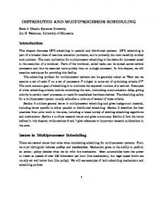
Fig. 15 and Fig. 16 give the contour graph of the density of the generated points in grayscale, where black is the maximum value and white is 0. The horizontal axis is Load LO , the vertical is Load HI . We used

(a) Density of Generated Jobs

(b) Schedulable by EDF-DS[1/2]

(c) Schedulable by MCPI

(d) Schedulable by MCPI and not by EDF-DS[1/2]

Figure 15: The contour graphs of random task graphs for 2 processors. The horizontal axis is Load LO , the vertical is Load HI . Load in the axes because it better reflects required parallelism. Figures from Fig. 15(a) to Fig. 15(d) refer to the experiments made for 2 processors. In particular Fig. 15(a) shows the density of the generated task graphs, Fig. 15(b) shows the percentage of instances schedulable by EDF-DS among the generated ones. Likewise Fig. 15(c) shows the percentage of task graphs schedulable by MCPI (EDF-DS) and Fig. 15(d) shows the percentage of task graphs schedulable by MCPI (EDF-DS) and not schedulable by EDF-DS. As expected the schedulability decreases while the distance from the axis origin increase. Fig. 15(d) is particularly interesting, because it shows how MCPI increases the schedulability over the support algorithm when the load increases. Notice that approximately around point (1.7, 1.7) the density is higher, suggesting that around this point MCPI is more effective. Figures from Fig. 16(a) to Fig. 16(d) show respectively the same information of figures from Fig. 15(a) to Fig. 15(d), but referred to experiments on 4 processors. From those graph we have confirmation of the conclusions made above. Also in Fig. 16(d) we have an area where MCPI is particularly effective, approximately around point (3.3, 3.1).

7

Conclusions

We addressed the problem of multi-processor scheduling of mixed criticality task graphs in synchronous systems. The advantage of our algorithm over state of the art was demonstrated by experiments on a large set of synthetic benchmarks, demonstrating a good improvement in schedulability.

Verimag Research Report no TR-2014-11

17/27

Dario Socci, Peter Poplavko, Saddek Bensalem, Marius Bozga

(a) Density of Generated Jobs

(b) Schedulable by EDF-DS[1/2]

(c) Schedulable by MCPI

(d) Schedulable by MCPI and not by EDF-DS[1/2]

Figure 16: The contour graphs of random task graphs for 4 processors. The horizontal axis is Load LO , the vertical is Load HI . In multi-processor scheduling is hard to apply the Audsley approach, previously proven effective for single-processor mixed-critical scheduling with precedence constraints [1]. Therefore in our algorithm, MCPI , we assign the priorities in a different order. Nevertheless, MCPI still generalizes an Audsleyapproach compliant algorithm MCEDF [7], when applied to single-processor instances without precedences. In future work, we plan to extend the algorithm for multiple criticality levels and to support pipelining.

References [1] S. Baruah, “Semantics-preserving implementation of multirate mixed-criticality synchronous programs,” in RTNS’12, pp. 11–19, ACM, 2012. 1, 5.2, 5.3, 5.3, 7 [2] J. Barhorst, T. Belote, P. Binns, J. Hoffman, J. Paunicka, P. Sarathy, J. Stanfill, D. Stuart, and R. Urzi, “White paper: A research agenda for mixed-criticality systems,” Apr. 2009. 1 [3] S. Baruah, V. Bonifaci, G. D’Angelo, H. Li, A. Marchetti-Spaccamela, N. Megow, and L. Stougie, “Scheduling real-time mixed-criticality jobs,” IEEE Trans. Comput., vol. 61, pp. 1140 –1152, aug. 2012. 1, 2.1, 2.1 [4] C. Ficek, N. Feiertag, and K. Richter, “Applying the AUTOSAR timing protection to build safe and efficient ISO 26262 mixed-criticality systems,” in ERTSS’2012, 2012. 1 [5] R. I. Davis and A. Burns, “A survey of hard real-time scheduling for multiprocessor systems,” ACM Comput. Surv., vol. 43, Oct. 2011. 1, 5.1

18/27

Verimag Research Report no TR-2014-11

Dario Socci, Peter Poplavko, Saddek Bensalem, Marius Bozga

[6] R. Ha and J. W. S. Liu, “Validating timing constraints in multiprocessor and distributed real-time systems,” in Proc. Int. Conf. Distributed Computing Systems, pp. 162–171, Jun 1994. 2.1 [7] D. Socci, P. Poplavko, S. Bensalem, and M. Bozga, “Mixed critical earliest deadline first,” in Euromicro Conf. on Real-Time Systems, ECRTS’13, pp. 93–102, IEEE, 2013. 2.1, 5.3, 6, 7, A, A.3 [8] J. W. S. Liu, Real-Time Systems. Prentice-Hall, Inc., 2000. 2.2 [9] S. Baruah and N. Fisher, “The partitioned multiprocessor scheduling of sporadic task systems,” in Real-Time Systems Symposium, 2005. RTSS 2005. 26th IEEE International, pp. 9 pp.–329, Dec 2005. 2.2 [10] H. Li and S. Baruah, “Load-based schedulability analysis of certifiable mixed-criticality systems,” in Intern. Conf. on Embedded Software, EMSOFT ’10, pp. 99–108, ACM, 2010. 2.2 [11] T. Park and S. Kim, “Dynamic scheduling algorithm and its schedulability analysis for certifiable dual-criticality systems,” in Intern. Conf. on Embedded software, EMSOFT ’11, pp. 253–262, ACM, 2011. 2.2 [12] Y.-K. Kwok and I. Ahmad, “Static scheduling algorithms for allocating directed task graphs to multiprocessors,” ACM Comput. Surv., vol. 31, pp. 406–471, Dec. 1999. 2.2, 5.2 [13] T. H. Cormen, C. Stein, R. L. Rivest, and C. E. Leiserson, Introduction to Algorithms. McGraw-Hill Higher Education, 2nd ed., 2001. 4.1, 4.1, 4.1 [14] S. K. Dhall and C. L. Liu, “On a real-time scheduling problem,” Operations Research, vol. 26, no. 1, pp. 127–140, 1978. 5.1 [15] S. K. Baruah, “Optimal utilization bounds for the fixed-priority scheduling of periodic task systems on identical multiprocessors,” IEEE Trans. Comput., vol. 53, pp. 781–784, June 2004. 5.1 [16] J. Forget et al., “Scheduling dependent periodic tasks without synchronization mechanisms,” in RTAS’10, pp. 301–310. 5.2 [17] H. Li and S. K. Baruah, “Outstanding paper award: Global mixed-criticality scheduling on multiprocessors,” in 24th Euromicro Conference on Real-Time Systems, ECRTS 2012, 2012. 5.3 [18] S. Baruah, “Implementing mixed-criticality synchronous reactive systems upon multiprocessor platforms.” 5.3 [19] E. Yip, M. Kuo, P. S. Roop, and D. Broman, “Relaxing the Synchronous Approach for MixedCriticality Systems,” in 12th IEEE Real-Time and Embedded Technology and Applications Symposium (RTAS), Apr. 2014. 5.3

Verimag Research Report no TR-2014-11

19/27

Dario Socci, Peter Poplavko, Saddek Bensalem, Marius Bozga

Appendices A

MCEDF and MCPI(EDF): Modifications and Optimality

In this appendix we formalize and prove Observation 5.1, which states that the MCEDF algorithm, proposed in [7], and a slightly modified MCPI(EDF) have equivalent schedulability. Note that because all these algorithms use LO-mode schedules to construct the priority tables, under the ‘scheduling’ we always mean the LO-mode scheduling unless mentioned otherwise.

A.1

Modified Version of MCPI

In this subsection we formulate a modified version of MCPI that is ‘closer’ to MCEDF. Additional experiments show results that are statistically indistinguishable from those of MCPI. In a later subsection we show that the modified MCis also equivalent to MCEDF, thus completing the argument of equivalence between MCPI and MCEDF. The modified version differs from MCPI by replacing subroutine MCPI PDAG by the subroutine modMCPI PDAG, shown in Figure 17. Also the PullUp subroutine is replaced by modPullup, where swap is defined differently. The modified MCPI is based on the following concept. Definition 4 (Potential Interference Relation). Given task graph T(J, →), number of processors m and a J0

subset J0 ⊆ J, we say that an equivalence relation ∼ on set J0 is a ‘potential interference’ relation if it has the following property: J0

∀J1 , J2 ∈ J0 . ∃P T : J1 `P T J2 ⇒ J1 ∼ J2 whereby we consider LO-mode m-processor list schedules on maximal task subgraph with nodes J0 . In modified MCPI we exploit the fact that if a potential interference relation is known then any two unrelated jobs can be kept in two different subtrees of a P-DAG even when one modifies the priorities in one of the subtrees, e.g., if one performs the priority swap operations. In general, there exist multiple potential interference relations, as joining two equivalence classes would lead to a new potential interference relation. Therefore, the (unique) maximal such relation is the total equivalence. The (unique) minimal potential interference relation can be obtained by union of blocking relations under all possible P T ’s, followed by transitive and reflexive closure, however it is a costly computation due to exponential number of P T ’s. Instead of computing this minimum, we over-approximate it by exploiting the following theorem (given without proof). Theorem A.1 (Single-Processor Interference). In preemptive list scheduling, a potential interference relation for single processor is also a potential interference relation for m processors. As it turns out (see the next section), calculating the minimal potential interference on a single processor can be done by a fast (almost linear) algorithm (the ‘makespan’). Therefore, we use the single-processor approximation, though it can be very rough one, and more refined approximations could be defined. Observation A.2 (Optimality Requirement on Interference Approximation). For the single-processor optimality results established in this section, the only requirement that we place on interference-relation over-approximation algorithm is that it gives the exact minimal interference relation at least for singleprocessor problem instances without precedence constraints (and which can be always ensured by using makespan). The modified MCPI algorithm differs from the original MCPI by the way it handles the HI jobs in the P-DAG construction. It employs a potential interference relation to try to put these jobs in separate sub-trees when pulling them up the P-DAG, reducing the ‘job-chaining’ in the P-DAG which we showed in Fig. 14. Note that the modified MCPI would behave exactly as the basic one if one used the worst

20/27

Verimag Research Report no TR-2014-11

Dario Socci, Peter Poplavko, Saddek Bensalem, Marius Bozga

1: 2: 3: 4: 5: 6: 7: 8: 9: 10: 11: 12: 13: 14: 15: 16: 17: 18: 19: 20: 21: 22:

Algorithm: modMCPI PDAG Input: task graph T(J, →) Input: priority table SP T In/out: forest P-DAG G(J0 , B) if J 6= ∅ then J curr ← SelectHighestPriorityJob(J, SP T ) ` ← SimulateListSchedule(LO, (G.J0 , →), PT(G) a J curr ) G.J0 ← G.J0 ∪ {J curr } for all trees ST ∈ G do if χ(J curr ) = LO then if ∃ J 0 ∈ ST : J 0 ` J curr ∨ J 0 → J curr then ConnectAsRoot(ST, J curr ) end if else J0 if ∃ J 0 ∈ ST : J 0 ∼ J curr ∨ J 0 → J curr then ConnectAsRoot(ST, J curr ) end if end if end for if χ(J curr ) = HI then modP ullU p(J curr , G, SP T ) modM CP I P DAG( T( J \ {J curr }, →), SP T, G(J0 , B)) end if Figure 17: The algorithm for computing P-DAG in MCPI - modified version

interference approximation (i.e., the total equivalence), but, obviously, such an approximation would not satisfy the optimality requirement in general. The P-DAG construction algorithm for the modified MCPI is shown in Figure 17. We see that the HI jobs now are connected only to the trees that may potentially interfere with them and hence also with each other when priorities are modified by the priority improvement. The modified priority improvement, modP ullU p calls a modified version of T reeSwap, denoted modT reeSwap. Definition 5 (Modified Swap). Let G(J0 , B) be a forest P-DAG, let JLO B JHI and let J00 represent the subset of jobs whose priorities can be potentially higher than or equal to JHI after the swap is performed: J00 = {JHI } ∪ {J 0 | J 0 B∗ JHI } \ {JLO } Subroutine modT reeSwap(JHI , JLO , G) performs the following ‘swap’ transformation on graph G: 1. JLO B JHI is transformed into JHI B JLO 2. ∀ tree ST : root(ST ) B JHI ∨ root(ST ) B JLO J00

(a) if ∃J 0 ∈ ST : J 0 ∼ JHI ∨ J 0 → JHI then in the new G: root(ST ) B JHI (b) else in the new G: root(ST ) B JLO 3. if ∃Js : JHI B Js then JHI B Js is transformed into JLO B Js The difference of the modified ‘swap’ operation from the basic version used by algorithm in Fig. 9 is only in the second rule above. The basic version does not distinguish the two cases in the second rule and always ‘plugs’ the subtrees ST into JHI . The modified version only plugs the subtree into JHI if after priority modifications the subtree can be involved in a blocking relation with JHI and/or other subtrees. Such a blocking relation would invalidate its property of being an independent tree in a P-DAG. If under no circumstances such a blocking relation can appear, the tree is plugged to the lower-priority job JLO . As a result, instead of a LO-job chain below the HI job shown in Fig. 14 we may see a stem to which side trees J00

may be plugged. Because, due to the check involving the ‘ ∼’ relation, the side subtrees can never block any job from the subtrees higher in the stem, the proposed modification to the swapping procedure may

Verimag Research Report no TR-2014-11

21/27

Dario Socci, Peter Poplavko, Saddek Bensalem, Marius Bozga

1: 2: 3: 4: 5: 6: 7: 8: 9: 10: 11: 12: 13:

Algorithm: modPullUp Input: job J Input: priority table SP T In/out: forest P-DAG G DON E = ∅ while LOpredecessors(J, G) 6= DON E do J 0 ← SelectLeastPriorityJob( ( LOpredecessors(J, G) \ DON E), SP T ) DON E ← DON E ∪ {J 0 } if CanSwap(J, J 0 , G) then modT reeSwap(J, J 0 , G) DON E ← DON E ∩ LOpredecessors(J, G) end if end while Figure 18: The modified pull-up subroutine

never lead to possible violations of the P-DAG property. Therefore, we adapt, without proof, Theorem 4.1 to the modified version of MCPI: Theorem A.3. The Graph produced by modMCPI PDAG procedure is a P-DAG. Moreover, after each basic step of the algorithm – the initial connection of a new job J curr and a tree swap – the intermediate graph G is a P-DAG as well. The modified P ullU p procedure, which exploits the new swap operation, is illustrated in Fig. 18. Unlike the basic P ullU p, Fig. 9, instead of keeping a list of predecessors that were not yet considered for swapping we keep its complement – the list of predecessors that have already been considered for swapping (‘done’). Like in the basic algorithm, we do not re-try to swap any such predecessor again, not even after another job has been swapped successfully. The main reason for this restriction is computational complexity, we would like to keep the worst case number of swap trials linear in the total number of jobs. Note that the modified algorithm can potentially directly connect two LO jobs by P-DAG edge that is incompatible with SP T priority order, which can happen if a swap will fail and another one will succeed. Note also that we use the same CanSwap procedure as before. We could have used a modified subroutine modCanSwap, which would differ from the basic CanSwap only in that it evaluates the schedulability of the P-DAG obtained from modified swap transformation, not the basic one. However, one can easily show that the schedulability of both P-DAGs is equivalent (because they differ only in the way they connect the non-interfering subtrees). However, as discussed earlier, the two different swapping methods result in different P-DAG structures, and, as we see in some examples, this may have essential effect on the HI jobs that are pulled through the same region of the P-DAG later than the current HI job.

A.2

Single-processor Scheduling and Busy Intervals

An important concept in the context of single-processor scheduling is busy interval. However, because this concept is better studied and understood for the case of no precedence constraints, we will define it using the notion of ‘modeling job set’. Definition 6 (Modeling job set). Given a task graph T(J, →), its modeling job set J∗ is the set of jobs whose arrival times are calculated as ASAP times A∗j for LO mode. Observation A.4 (Modeling job set identity when no precedences). The modeling job set is identical to the original job set if the task graph has no precedence edges. Definition 7 (Predecessor-closed subset). Given a task graph T(J, →), a subset of jobs J0 ⊆ J is predecessor-closed if including a job in this subset implies including all its predecessors. The following theorem is given without proof:

22/27

Verimag Research Report no TR-2014-11

Dario Socci, Peter Poplavko, Saddek Bensalem, Marius Bozga

Theorem A.5 (Modeling list schedule by fixed priority). Given a predecessor-closed subset and considering single processor schedules, then using any priority table that is priority-compliant one gets the same basic LO scenario schedules from: 1. the list scheduling of the corresponding maximal subgraph 2. fixed-priority scheduling of the corresponding modeling subset Definition 8 (Busy Interval). A busy interval for a predecessor-closed subset of jobs J0 is a time interval in a fixed-priority schedule for the corresponding modeling job subset J0∗ . It is defined as a maximal time interval (τ1 , τ2 ] where at least job is ready for execution. By abuse of terminology, we apply the term ‘busy interval’ also to the subset of jobs running in that interval, and denote it BI. Note that the time interval in the definition is half-open because the jobs that arrive at time t count ready only for the time instances strictly later than t. It is obvious that on a single processor either the start time nor the length of a busy interval depends on the exact priority assignment, because the former corresponds to the earliest job arrival and the latter is equal to the sum of Ci (LO) of all jobs in the interval. In general, a job set J0 can be partitioned into multiple BI subsets, because some jobs may arrive at or later than the end of a busy interval of some other jobs. To calculate the busy intervals one can simulate the fixed-priority policy on the modeling job set for any priority table and apply the definition of busy interval to find the time bounds and the contents of job subsets that belong to the same busy interval. The following lemma is easy to prove: Lemma A.6 (Least priority in a busy interval). Given a job set J0 and any of its busy interval BI with time interval (τ1 , τ2 ]. In fixed-priority scheduling for job set J0 , the least-priority job running in this BI terminates at time τ2 and is blocked by at least one other job in BI (if there are any). The following theorem can be easily derived from the above lemma: Theorem A.7 (Minimal Potential Interference in Busy Intervals). Given a job set J0 without precedences, then the set of busy intervals BI are the equivalence classes of the corresponding minimal potential interJ0

ference relation ∼ on single processor. Corollary A.8 (Potential interference with precedences). Given a task graph and a predecessor-closed subset of jobs J0 . The set of busy intervals BI correspond to equivalence classes of some (not necessarily J0

minimal) potential interference relation ∼ on single processor. We cannot claim minimality in the second case above because currently we are not sure about it. Observation A.9 (Implementation of Modified MCPI based on Busy Intervals). It can be easily shown J0

that modified MCPI evaluates relation ∼ only for predecessor-closed subsets. Therefore, it can use busy intervals for this evaluation. Because to obtain busy intervals one requires to do just one extra simulation for a subset of jobs where at least one simulation needs to be done anyway, the modified MCPI based on busy intervals has the same computational complexity as the basic MCPI. Moreover, by the theorem above, busy intervals satisfy our requirement of giving exact evaluation of the minimal single-processor interference for the case without precedence constraints.

A.3

Recalling the MCEDF Algorithm

MCEDF is defined, which are, compared to the assumptions of this paper, restricted in two different ways: (1) assume single processor platform, m = 1 (2) assume no precedence between jobs, →= ∅ Due to the second restriction, we consider just job sets J rather than task graphs T as problem instances, and simple fixed-priority policy instead of list scheduling. In this section we recall the definition of MCEDF from [7], while adapting this description to the terminology and notations of this paper.

Verimag Research Report no TR-2014-11

23/27

Dario Socci, Peter Poplavko, Saddek Bensalem, Marius Bozga

Algorithm: MCEDF PDAG Input: job set J Input: node Jparent 4: In/out: P-DAG G 5: Input: EDF-compliant priority table SP T

1: 2: 3:

6: 7: 8: 9: 10: 11: 12: 13: 14: 15: 16:

B ← PartitionIntoBIs(J); for all BI ∈ B do J least ← AssignJobLeastPriority(BI, SP T ) G.J ← G.J ∪ {J least } if Jparent 6= ∅ then G. B ← G. B ∪ {(J least , Jparent )} end if J0 ← BI \ {J least } M CEDF P DAG(J0 , J least , G) end for Figure 19: The MCEDF algorithm for computing P-DAG

The MCEDF algorithm has the same basic structure as MCPI. The top-level structure of MCEDF basically repeats that of MCPI given in Fig. 6, except that it does not need to call PTTransform. Though it is not explicit in the original description of MCEDF, similarly to MCPI, it also uses a support priority table SP T . The point is that it requires that SP T must be EDF-compliant, but if all jobs have different deadlines (which is often the case) than there exists only one unique such table for the given job set. For the theoretical properties studied in [7] the choice of the particular EDF-compliant table does not have an influence, but in this description we emphasize the SP T table as are final goal is to prove the equivalence of (modified) MCPI and MCEDF under the condition that they use the same SP T . Though, like modified MCPI, MCEDF also employs busy intervals, it uses an essentially different algorithm for constructing the P-DAG, shown as subroutine MCEDF PDAG in Figure 19. The P-DAG construction algorithm splits the instance into BI’s and assigns one of the jobs in each BI the least priority. Recall from Lemma A.6, that in a busy interval (τ1 , τ2 ], the job assigned the least priority will complete at time τ2 . low and JHIlow , which are the least The two candidates to be assigned the least priority by MCEDF are JLO SP T -priority jobs LO resp. HI jobs among those in the busy interval. Note that since the SP T table is EDF compliant, those two jobs are also latest-deadline among the LO resp. HI jobs present in the given BI. Subroutine AssignJobLeastPriority selects the least priority job according to the following rule. low • if ∃Jj ∈ BI : χj = LO ∧ JLO .D ≥ τ2 low • then J least ← JLO

• else J least ← JHIlow low This rule prefers to assign the least priority to JLO if BI has some LO jobs and if a latest-deadline one among them would not miss its deadline. Otherwise the algorithm has no other choice but to select a HI job. Thus, the algorithm greedily avoids assigning a HI job the least priority, and does so only when this cannot be avoided. Intuitively, this is similar to trying to pull a HI job as high as possible in the P-DAG in the context of MCPI. After assigning the least priority in the given BI the algorithm continues recursively with sub-instances J0 = BI \ {J least }. Removing a job from a BI reveals further fragmentation into busy intervals, which become direct children of BI in the P-DAG. In those new BI’s the same algorithm is used to find the least-priority job and to construct the subtree further from the roots to the leafs. The final G P-DAG of the MCEDF algorithm has multiple subtrees whose root nodes correspond to the BI’s of the complete problem instance J. If we consider each subtree separately as a subset J0 and

24/27

Verimag Research Report no TR-2014-11

Dario Socci, Peter Poplavko, Saddek Bensalem, Marius Bozga

remove the root of the subtree from the subset, then, by construction, different children of the root would correspond to the busy intervals of the given subset. We can consider this process again and again and will see further fragmentation into busy intervals of jobs that have a higher priority than the root of the subtree.

A.4

The Properties of MCEDF and the Modified MCPI

In this subsection under MCPI will always mean the modified version of MCPI and we assume that both algorithms use the same EDF-compliant support priority table SP T . The following lemma establishes for MCPI a property that is true for MCEDF by construction. Lemma A.10. In MCPI, as in MCEDF, each tree of the P-DAG contains jobs from one and only one busy interval. Proof. (sketch) For MCPI, we argue that this property is true by demonstrating that at each basic step of the algorithm: the initial connection of a new job to the P-DAG and the swapping. When a LO-job is connected to a P-DAG, the criterion is to connect it to the trees that block the given job when it has the least priority. Since they block the given job then they must be in the same busy interval. When a HI job is initially connected, the property holds by construction, as we use splitting into busy intervals to evaluate J0

∼. Now consider the swapping. After the swapping, the current HI job forms one same busy interval with the subtrees connected to it by the same argument as the ones we used for the initial connection. The LO job which was swapped forms one busy interval with the current HI job tree and other trees that are plugged to it by observation that this was already the case before the swap and the busy intervals do not change when priority assignment changes. Lemma A.11 (Per-criticality EDF Compliance of P-DAG). In the P-DAG G of MCPI(EDF) or MCEDF, consider any P-DAG path between two jobs of the same criticality: Ji B∗ Jj . This path can only join Ji and Jj in the direction that is compliant with their relative priority in SP T . Mathematically: ∀i, j . χi = χj ∧ Ji B∗ Jj ⇒ Ji SP T Jj

(11)

Proof. (sketch) For MCEDF the Property (11) holds by construction, as it requires that Jj be the root of a subtree that contains Ji and MCEDF PDAG assigns the least SP T -priority job of a given criticality as the root of the subtree. For MCPI, as P-DAG construction evolves, the property can only be potentially broken by the swap operations. However, for criticality level HI it is not broken because we never swap two HI jobs. For criticality LO it can be only invalidated if CanSwap never returns ‘false’ and then ‘true’ in the same P ullU p subroutine call. This is so because the LO jobs are evaluated for swapping in an order compliant with reverse SP T and the stem of swapped jobs forms a chain in the same order as the swapping is done. The job for which CanSwap would return ‘false’ would stay as predecessor of the current HI job and the job with ‘true’ would become successor, thus forming a pair of LO jobs connected inconsistently with SP T . However, this cannot happen if SP T is EDF-compliant, as the first ‘false’ result from CanSwap will be followed by other ‘false’. To show this, recall that by Lemma A.10 the HI job forms one busy interval (τ1 , τ2 ] with its subtree. When CanSwap evaluates different LO jobs for the least priority it evaluates for the possibility that the swapped job can terminate at time τ2 while meeting its deadline. The jobs are evaluated in reverse EDF order, so the job with the largest deadline will be evaluated first. However, if that job misses its deadline at time τ2 then the other jobs will fail as well. By the above lemma, for MCEDF and MCPI(EDF), it is always possible to find a topological sort of graph G such that the resulting priority table satisfies the following property: Definition 9 (HI-criticality EDF Compliance of Priority Table). Given an EDF-compliant SP T priority table, any LO-mode priority table P T is said to be HI-criticality EDF-compliant according to table SP T if the HI jobs appear in P T in the same order as in SP T , that is: ∀i, j . χi = χj = HI ∧ Ji P T Jj

Verimag Research Report no TR-2014-11

⇒ Ji SP T Jj ∧ Di ≤ Dj

25/27

Dario Socci, Peter Poplavko, Saddek Bensalem, Marius Bozga

Consider a problem instance J where h jobs are HI-critical. We can partition an EDF-compliant priority table generated by MCEDF/MCPI(EDF) into the following sequence of job sets: LO LO LO HI HI HI P T : JLO 1 P T {J1 } P T J2 P T {J2 } P T . . . Jh P T {Jh } P T Jh+1

HI jobs : J1 SP T J2 SP T . . . Jh−1 SP T Jh HI

HI

HI

HI

(12a) (12b)

where subscript l and h denote LO and HI jobs and relation ‘’ between two job sets means that any job in the first set has a higher priority than any job in the second set. Let us denote by B∗LO a relation between two jobs that are joined in the P-DAG by a path that may have only LO jobs as intermediate nodes. The following is trivial: Lemma A.12. There always exists a priority table P T obtained from a topological sort of P-DAG G of MCEDF or MCPI(EDF) that has the structure shown in Formulas (12) where, in addition, the LO job sets ∗LO HI : JLO i are defined as the sets of LO jobs related to Ji by B ∗LO HI Ji } for i = 1..h . JLO i = {Jj | χj = LO ∧ Jj B ∗LO HI Ji } JLO h+1 = {Jj | χj = LO ∧ 6 ∃i : Jj B

(13a) (13b)

Definition 10 (A Least LO-Priority Table). Given a P-DAG G that is per-criticality compliant to support priority table SP T . A priority table obtained from graph G that can be partitioned as shown in Formulas (12) and (13) is called a least LO-priority table. The reason to give a priority table this name is that such a table puts each LO job at the highest-i (and hence also the least-priority) set JLO i . The following lemma states that one cannot give any LO job even less priority w.r.t. a HI job. Lemma A.13. Let J be a problem instance where MCEDF or MCPI(EDF) generates a P-DAG based on 0 an EDF-compliant SP T , let JLO i characterize its least LO-priority table. Let P T be a HI-criticality SP T LO compliant priority table where some LO jobs in some job sets Ji ‘violate the least LO priority constraint’ in the sense that they have a less priority than the corresponding HI job JiHI . Then at least one of such jobs will miss its deadline. Proof. Let i0 be the smallest-index i of the job sets JLO i that contain ‘violating’ LO jobs in the sense defined the in lemma conditions. Let Jj be the least-priority violating job from that set. Let us show that it will miss its deadline. The part of the priority table P T 0 that contains jobs of priority higher or equal to Jj can be represented by (dropping the curly braces for singleton sets): P T 0 |j : J0 1  J1HI  . . .  J0 i0 −1  JiHI0 −1  J0 i0  JiHI0  J00 i0  Jj Observing that in single processor scheduling the relative priority order of higher-priority jobs does not matter for the least priority job, let us reorder the priority of the last HI job and obtain table P T 00 that results in equal termination time for job Jj : P T 00 : J0 1  J1HI  . . .  J0 i0 −1  JiHI0 −1  J0 i0  J00 i0  JiHI0  Jj 0 From the definition of violating jobs and from the assumption that the sets JLO m for m ≤ i − 1 contain no 0 violating jobs (i being the lowest ‘violating’ index) we have: 0 for 1 ≤ m ≤ i0 − 1 : JLO m ⊆J m

Also because, by our assumptions, Jj is the least priority violating job in set i0 we have: 0 00 JLO i0 ⊆ (J i0 ∪ J i0 ∪ {Jj })

By the job-set inclusion relation above, the following priority table P T 000 when compared to P T 00 has at most the same but possibly less jobs of higher-priority than Jj : LO LO HI HI HI P T 000 : JLO 1  J1  . . .  Ji0 −1  Ji0 −1  (Ji0 \ Jj )  Ji0  Jj

26/27

Verimag Research Report no TR-2014-11

Dario Socci, Peter Poplavko, Saddek Bensalem, Marius Bozga

By properties of MCEDF resp. MCPI(EDF) we have that job JiHI0 forms one busy interval BI with the higher subtrees connected to it and by observation that Jj B∗LO JiHI0 also belongs to the same busy interval BI. Now observe that the reason why MCEDF resp. MCPI(EDF) assigned JiHI0 the least priority in the given BI is because the highest-deadline LO job belonging to the same interval would miss the deadline. Jj , by construction, cannot have a higher deadline, so it should also miss its deadline as the least-priority job in BI. Therefore it will also miss its deadline in P T 000 , and hence also in P T 00 and P T 0 . We can now prove the following: Theorem A.14. For a given EDF-compliant SP T , MCEDF and MCPI(EDF) are optimal among the FPM algorithms that are HI-criticality EDF-compliant according to SP T . Proof. (sketch) First, note that if an instance J is MC-Schedulable, then the MCEDF and MCPI(EDF) algorithms will never fail in LO mode and produce a P-DAG that conforms to the lemma’s and properties presented in this section. This is so because, firstly, both algorithms are based on iterative improvement of an EDF table, which is optimal in the LO mode. Secondly, at every improvement step the LO-schedulability of the problem instance is preserved as an invariant. This leads to two important conclusions: 1. The only possible schedulability failure that MCEDF or MCPI(EDF) can have is when a HI job that misses its deadline in a HI scenario. 2. For MC-schedulable instance, even if we see the worst case presented in point 1, both algorithms manage to construct a LO-schedulable P-DAG that satisfies all lemma’s and properties presented in this section. Consider an instance J with h HI jobs. Suppose by contradiction that MCEDF resp. MCPI(EDF) fail to produce a feasible schedule due to a failure in a HI scenario, whereas the optimal algorithm can. By lemma’s above, we can present the solution of both algorithms as shown in Formulas (12) and (13). The theorem conditions require that priority tables be HI-criticality EDF-compatible according to SP T , so the optimal priority table P T 0 can also be presented in a similar form: P T 0 : J0 1  {J1HI }  J0 2  {J2HI }  . . . J0 h  {JhHI }  J0 h+1 By Lemma A.13 we should have: for 1 ≤ m ≤ h :

m [

JLO i ⊆

i=1

m [

J0 i

i=1

where JLO m are the least LO-priority job sets of MCEDF resp. MCPI(EDF). HI This means that, compared to MCEDF or MCPI(EDF), for every HI job Jm the optimal algorithm puts HI at least the same but possibly a larger set of jobs as higher-priority w.r.t. to Jm . On a single processor this can only decrease the progress made by each HI jobs up to any given point in time in the LO mode. Therefore, after a mode switch, all the HI jobs in the optimal algorithm will have at least the same or possibly more workload to complete than in MCEDF or MCPI(EDF). Therefore, if the latter would fail in some HI scenario all the more so the former would also fail in the same scenario, therefore the optimal algorithm would fail and thus we have a contradiction. The next theorem follows as a corollary of Theorem A.14: Theorem A.15. When using the same EDF-compatible SP T table MCEDF and MCPI(EDF) are equivalent. Note that, despite equivalence, MCEDF has a lower computational complexity, O(k 2 log k), than MCPI, which has O(k 3 log k) (where k is the number of jobs). Intuitively, this is so because MCEDF is ‘specialized’ for the single-processor scheduling problems, which is inherently ‘simpler’ than the multiprocessor ones, handled by MCPI.

Verimag Research Report no TR-2014-11

27/27