Many-to-Many Graph Matching via Metric Embedding - University of

Many-to-Many Graph Matching via Metric Embedding Yakov Keselman DePaul University

Ali Shokoufandeh Drexel University

Abstract Graph matching is an important component in many object recognition algorithms. Although most graph matching algorithms seek a one-to-one correspondence between nodes, it is often the case that a more meaningful correspondence exists between a cluster of nodes in one graph and a cluster of nodes in the other. We present a matching algorithm that establishes many-to-many correspondences between nodes of noisy, vertex-labeled weighted graphs. The algorithm is based on recent developments in efficient lowdistortion metric embedding of graphs into normed vector spaces. By embedding weighted graphs into normed vector spaces, we reduce the problem of many-to-many graph matching to that of computing a distribution-based distance measure between graph embeddings. We use a specific measure, the Earth Mover’s Distance, to compute distances between sets of weighted vectors. Empirical evaluation of the algorithm on an extensive set of recognition trials demonstrates both the robustness and efficiency of the overall approach.

1. Introduction The problem of object recognition is often formulated as that of matching configurations of image features to configurations of model features. Such configurations are often represented as vertex-labeled graphs, whose nodes represent image features (or their abstractions), and whose edges represent relations (or constraints) between the features. The relations are typically geometric or hierarchical, but can include other types of information. To match two graph representations means to establish correspondences between their nodes. To evaluate the quality of a match, one defines an overall distance measure, whose value depends on both node and edge similarity. Due to the importance of the recognition problem (forThe work of Yakov Keselman is supported in part by the NSF grant No. 0125068. Ali Shokoufandeh acknowledges the partial support provided by grant ITR-DM-0219176 from NSF. Sven Dickinson acknowledges the support of NSERC and NSF.

M. Fatih Demirci Drexel University

Sven Dickinson University of Toronto

mulated in terms of graph matching), there has been a growing interest in developing efficient algorithms for matching vertex-labeled graphs. Previous work on graph matching (see Section 2) has typically focused on the problem of finding a one-to-one correspondence between the vertices of two graphs. However, the assumption of one-to-one correspondence is a very restrictive one, for it assumes that the primitive features (nodes) in the two graphs agree in their level of abstraction. Unfortunately, there are a variety of conditions that may lead to graphs that represent visually similar image feature configurations yet do not contain a single one-to-one node correspondence. For example, due to noise or segmentation errors, a single feature (node) in one graph may map to a collection of broken features (nodes) in another graph. Or, due to scale differences, a single, coarse-grained feature in one graph may map to a collection of fine-grained features in another graph. In general, we seek not a one-to-one correspondence between image features (nodes), but rather a many-to-many correspondence. Several existing approaches to the problem of manyto-many graph matching suffer from computational inefficiency and/or from an inability to handle small perturbations in graph structure. This paper seeks a solution to this problem while addressing drawbacks of existing approaches. Drawing on recently-developed techniques from the domain of low-distortion graph embedding, we have explored an efficient method for mapping a graph’s structure to a set of vectors in a low-dimensional space. This mapping not only simplifies the original graph representation, but it retains important information about both local (neighborhood) as well as global graph structure. Moreover, the mapping is stable with respect to noise in the graph structure. Armed with a low-dimensional, robust vector representation of an input graph’s structure, many-to-many graph matching can now be reduced to the much simpler problem of matching weighted distributions of points in a normed vector space, using a distribution-based similarity measure. We consider one such similarity measure, known as the Earth Mover’s Distance, and show that the many-to-many vector mapping that realizes the minimum Earth Mover’s

Distance corresponds to the desired many-to-many matching between nodes of the original graphs. The result is a more efficient and more stable approach to many-to-many graph matching that, in fact, includes the special case of one-to-one graph matching. To illustrate the approach, we apply it to the problem of view-based object recognition, in which views are represented as skeleton graphs.

2. Related Work The problem of object recognition is often formulated as that of matching feature graphs. Several researchers have developed algorithms that find one-to-one correspondences between graph nodes. Shapiro and Haralick [21] proposed a matching algorithm based on comparing weighted primitives (weighted attributes and weighted relation tuples) using a normalized distance for each primitive property that is inexactly matched. Kim and Kak [9] used a combination of discrete relaxation and bipartite matching in modelbased 3-D object recognition. Pellilo et al. [16] devised a quadratic programming framework for matching association graphs using a maximal clique formulation, while Gold and Rangarajan [6] used graduated assignment for matching graphs derived from feature points and image curves. Siddiqi et al. combined a bipartite matching framework with a spectral decomposition of graph structure to match shock graphs [23], while Shokoufandeh et al. [22] extended this framework to directed acyclic graphs that arise in multiscale image representations. Hancock and his colleagues have also proposed numerous frameworks for graph matching, including [14]. The problem of many-to-many graph matching has also been studied, most often in the context of edit-distance (see, e.g., [13, 20]). In such a setting, one seeks a minimal set of relabelings, additions, deletions, merges, and splits of nodes and edges that transform one graph into another. However, the edit-distance approach has its drawbacks: 1) it is computationally expensive (polynomial-time algorithms are available only for trees); 2) the method in its current form does not accommodate edge weights; and 3) the cost of an editing operation often fails to reflect the underlying visual information (for example, the visual similarity of a contour and its corresponding broken fragments should not be penalized by the high cost of merging the many fragments). In the context of line and segment matching, Beveridge and Riseman [3] addressed this problem via exhaustive local search. Although their method found good matches reliably and efficiently (due to their choice of the objective function and a small neighborhood size), it is unclear how this can be generalized to other types of feature graphs and objective functions. In a novel generalization of Scott and Longuet [19], Kosinov and Caelli [10] showed how inexact graph match-

ing can be solved using the re-normalization of projections of vertices into the eigenspaces of graphs along with a form of relational clustering. In [17] Pelillo et. al. generalized their replicator dynamical systems for attributed tree matching using the notion of -morphism (a many-to-one mapping). This construct allowed them to build an association graph where maximal weight cliques are in one-toone correspondence with maximal similarity subtree morphisms. In relation to low-distortion metric representations of graphs, Indyk [8] provides a comprehensive survey of recent advances and applications of low-distortion graph embedding. For recent results related to the properties of lowdistortion tree embedding, see [12, 1, 15].

3. Metric Embedding of Graphs During the last decade, low-distortion embedding has become recognized as a very powerful tool for designing efficient algorithms. In low-distortion embedding of metric spaces into normed spaces, we consider mappings , where is a set of points in the original met, is a set of points ric space, with distance function in the (host) -dimensional normed space , and for any we have pair , for a certain parameter , known as the distortion. Intuitively, such an embedding will enable us to re, duce problems defined over difficult metric spaces, to problems over easier normed spaces, . Clearly, the closer is to , the better the target set mimics the original set . Consequently, the distortion parameter is a critical characteristic of embedding . Perhaps the most fundamental existence result in computational embedding is due to Bourgain [4]: can be embedded Lemma 1 Any finite metric space of dimension at most into a finite normed space with distortion . This result is important since even an exponential 1 matching algorithm in the normed space may be tractable. However, distortion is too high; we seek an embedding with a much lower distortion.

3.1. Low-Distortion Embedding Our interest in low-distortion embedding is motivated by its ability to transform the problem of many-to-many matching in finite graphs to geometrical problems in low-dimensional vector spaces. Specifically, let , denote two graphs on vertex sets and , edge sets and , under disand , respectively ( represents the tance metrics 1 in

the dimension of the target space.

distances between all pairs of nodes in ). Ideally, we seek a single embedding that can map each graph to the same vector space, in which the two embeddings can be directly compared. However, in general, this is not possible without introducing unacceptable distortion. We will therefore tackle the problem in two steps. First, we will seek low-distortion embeddings that map sets to normed spaces , . Next, we will align the normed spaces, so that the embeddings can be directly compared. Using these mappings, the problem of manyand is therefore to-many vertex matching between reduced to that of computing a mapping between subsets and . of In practice, the robustness and efficiency of mapping will depend on several parameters, such as the magnitudes of distortion of the ’s under the embeddings, the computational complexity of applying the embeddings, the efficiency of computing the actual correspondences (including and , and the quality alignment) between subsets of of the computed correspondence. The latter issue will be addressed in Section 4. The problem of low-distortion embedding has a long history for the case of planar graphs, in general, and trees, in particular. More formally, the most desired embedding is the subject of the following conjecture: be a planar graph, and Conjecture 1 [7] Let let be the shortest-path metric for the graph . Then there is an embedding of into with distortion. This conjecture has only been proven for the case in which is a tree. Although the existence of such a distortion-free embedding under -norms was established in [11], no deterministic construction was provided. One such deterministic construction was given by Matou˘sek [15], suggesting that if we could somehow map our graphs into trees, with small distortion, we could adopt Matou˘sek’s framework.

3.2. The Shortest Path Metric Before we can proceed with Matou˘sek’s embedding, we must choose a suitable metric for our graphs, i.e., we must define a distance between any two vertices. Let denote an edge-weighted graph with real edge weights , . We will say that is a metric for if, , , for any three vertices , and . In general, there are many ways to define metric distances on a weighted graph. The best-known metric is the shortest-path , i.e., , the shortest path dismetric . In fact, if the tance between and for all weighted graph is a tree, the shortest path between any

two vertices is unique, and the weights of shortest paths be. tween any two vertices will define a metric can be defined In the event that is not a tree, through a special representation of , known as the centroid metric tree [1]. The path-length between any two vertices in will mimic the metric in . A on objects is a centroid metmetric ric if there exist labels such that for all , . If is not a tree, its centroid metric and weighted edgetree is a star on vertex-set set . It is easy to see that the path-lengths between and in will correspond to in . For details on the construction of a metric labeling of a metric distance see [1].

3.3. Path Partition of a Graph The construction of the embedding depends on the notion of a path partition of a graph. In this subsection, we introduce the path partition, and then use it in the next subsection to construct the embedding. Given a weighted graph with metric distance , let denote a tree representation of , whose vertex distances are . In the event that is a tree, ; consistent with otherwise is the centroid metric tree of . To construct the embedding, we will assume that is a rooted tree. It will be clear from the construction that the choice of the root does not affect distortion of the embedding. The dimensionality of the embedding of depends on the caterpillar dimension, denoted by , and is recursively defined as follows [15]. If consists of a single vertex, we set . For a tree with at least 2 vertices, if there exist paths beginning at the root and otherwise pairwise disjoint, such that of sateach component . Here isfies denotes the tree with the edges of the ’s removed, and the components are rooted at the single vertex lying on some . The caterpillar dimension can be determined in linear time for a rooted tree , and it is known that (see [15]). , for , depends The construction of vectors on the notion of a path partition of . The path partition of is empty if is single vertex; otherwise consists of some paths as in the definition of , plus the union of path partitions of the components of . The paths have are the paths of level level 1, and the paths of level in the corresponding path partitions of the components of . Note that the paths in a path partition are edge-disjoint, and their union covers the edge-set of . To illustrate these concepts, consider the tree shown in

Level 1 Level 2

Figure 1. Path partition of a tree. Figure 1. The three darkened paths from the root represent three level 1 paths. Following the removal of the level 1 paths, we are left with 6 connected components that, in turn, induce seven level 2 paths, shown with lightened edges. 2 Following the removal of the seven level 2 paths, we are left with an empty graph. Hence, the caterpillar dimension ) is 2. It is easy to see that the path partition can ( be constructed using a modified depth-first search in time.

3.4. Construction of the Embedding Given a path partition of , we will use to denote represent the unique the number of levels in , and let path between the root and a vertex . The first segment of of weight follows some path of level 1 in , of level the second segment of weight follows a path 2, and the last segment of weight follows a path of level . The sequences and will be referred to as the decomposition sequence and the weight sequence of , respectively. under , we To define the embedding let the relevant coordinates in be indexed by the paths in . The vector , , has non-zero coordinates corresponding to the paths in the decomposition sequence . Returning to Figure 1, the vector will have of 10 components (defined by three level 1 paths and seven will have at level 2 paths). Furthermore, every vector most two non-zero components. Consider, for example, the lowest leaf node in the middle branch. Its path to the root will traverse three level 2 edges corresponding to the fourth level 2 path, as well as three level 1 edges corresponding to the second level 1 path. Such embedding functions have become fairly standard in the metric space representation of weighted graphs [12, 15]. In fact, Matou˘sek [15] has proven that setting the -th coordinate of , corresponding to path , , , to in decomposition sequence

will result in a small distortion of at most 2 Note

. It

that the third node from the root in the middle level 1 branch is the root of a tree-component consisting of five nodes that will generate two level 2 paths.

should be mentioned that although the choice of path decomposition is not unique, the resulting embeddings are isomorphic up to a transformation. Computationally, conand structions of , , and are all linear in terms of . The above embedding has preserved both graph structure and edge weights, but has not accounted for node information. To accommodate node information in our embedding, to each vector , for all we will associate a weight . These weights will be defined in terms of vertex labels which, in turn, encode image feature values. Note that nodes with multiple feature values give raise to a vector of weights assigned to every point. We will present an example of one such distribution in Section 4.4.

4. Distribution-based Matching By embedding vertex-labeled graphs into normed spaces, we have reduced the problem of many-to-many matching of graphs to that of many-to-many matching of weighted distributions of points in normed spaces. However, before we can match two point distributions, we must map them into the same normed space. This involves reducing the dimension of the higher-dimensional distribution and transforming one of the distributions with respect to the other. Given a pair of weighted distributions in the same normed space, the Earth Mover’s Distance (EMD) framework [18] is then applied to find an optimal match between the distributions. The EMD approach computes the minimum amount of work (defined in terms of displacements of the masses associated with points) it takes to transform one distribution into another.

4.1. Embedding Point Distributions in the Same Normed Space Embeddings produced by the graph embedding algorithm can be of different dimensions and are defined only up to a distance-preserving transformation (a translated and rotated version of a graph embedding will also be a graph embedding). Therefore, in order to apply the EMD framework, we must first perform a “registration” step, whose objective is to project the two distributions into the same normed space. The resulting transformation is expected to minimize the initial EMD between the distributions. Our transformation is based on Principal Component Analysis (PCA). Namely, the projection of the original vectors onto the subspace spanned by the first right singular vectors of the covariance matrix retains the maximum information about the original vectors among all projections onto subspaces of dimension . Hence, projecting the two distributions onto the first right singular vectors of their covariance matrices will equalize their dimensions while los-

ing minimal information. Specifically, assuming that is the minimum of the two dimensions, we define embeddings and as follows:

first

is the SVD of columns of

first

is the SVD of columns of

4.2. The Earth Mover’s Distance The Earth Mover’s Distance (EMD) [18, 5] is designed to evaluate dissimilarity between two multi-dimensional distributions in some feature space. The EMD approach assumes that a distance measure between single features, called the ground distance, is given. The EMD then “lifts” this distance from individual features to full distributions. Moreover, if the weights of distributions are the same, and the ground distance is a metric, EMD induces a metric distance [18]. However, the main advantage of using EMD lies in the fact that it subsumes many histogram distances and permits partial matches in a natural way. This important property allows the similarity measure to deal with uneven clusters and noisy datasets. Computing the EMD is based on a solution to the wellknown transportation problem [2], whose optimal value determines the minimum amount of “work” required to transform one distribution into the other. More formally, let be the first distribution with points, and let be be the the second distribution with points. Let ground distance matrix, where is the ground distance between points and . Our objective is to find a flow , with being the flow between points matrix and , that minimizes the overall cost:

The above formulation assumes that the two distributions have been aligned. However, recall that a translated and rotated version of a graph embedding will also be a graph embedding. To accommodate pairs of distributions that are “not rigidly embedded”, Cohen and Guibas [5] extended the definition of EMD, originally applicable to pairs of fixed sets of points, to allow one of the sets to undergo a transformation. Assuming that a transformation is applied to the second distribution, distances are defined as , and the objective function be. The mincomes Work imal value of the objective function Work defines the Earth Mover’s Distance between the two distributions that are allowed to undergo a transformation from . Cohen and Guibas [5] also suggested an iterative process (which they call FT, short for “an optimal Flow and an optimal Transformation”) that achieves a local minimum of the objective function. Starting with an initial transfrom a given , they comformation pute the optimal flow that minimizes the objective function Work , and from a given opthey compute an optimal transformation timal flow that minimizes the objective function . The iterative process stops when the Work improvement in the objective function value falls below a threshold. The resulting optimal pair depends on the . Starting the iteration from sevinitial transformation eral initial transformations increases the likelihood of obtaining a global minimum.

4.3. Choosing an Appropriate Transformation For our application, the set of allowable transformations consists of only those transformations that preserve distances. Therefore, we use a weighted version of the Least Squares Estimation algorithm [24] to compute an optimal distance-preserving transformation given a flow between the distributions. Specifically, given a set of pairings (the flow of weight is sent from point to point ), we define the transformation in accordance with [24] as follows:

Work subject to the following list of constraints:

, where

The optimal value of the objective function Work defines the Earth Mover’s Distance between the two distributions.

is the SVD of

The original proof of optimality of the transformation [24] is easily adapted to the weighted case. Namely,

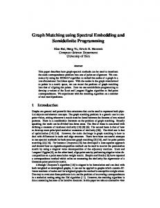
Figure 2. Left: the silhouette and its medial axis. Right: the medial axis tree constructed from the medial axis. Darker nodes reflect larger radii. assuming that the flows from the ’s to the ’s are integer, each weighted pairing is replaced by unweighted pairings , which makes the original proof applicable. Collecting appropriate terms, we get weighted versions of the original equations. Fractional flows are reduced to integer flows by multiplying all fractions by their least common denominator.

4.4. The Final Algorithm Our algorithm for many-to-many matching is a combination of the previous procedures. Specifically, given two vertex-labeled graphs and , we first find lowdistortion embeddings of the graphs into low-dimensional normed spaces, obtaining two weighted distributions. We then “register” one distribution with respect to the other so as to minimize the (original) EMD between them. We then apply the FT iteration of the transformation version of the EMD framework [5] to minimize the (extended) EMD. The pairing of points minimizing the EMD corresponds to a weighted many-to-many pairing of nodes. We summarize our approach in Algorithm 1. Algorithm 1 Many-to-many graph matching 1: Construct low-distortion embeddings of into ) according to Section 3.4. 2: Compute low-distortion embeddings into ) according to Section 4.1. 3: Compute the EMD between ’s by applying the FT iteration (Section 4.2), computing the optimal transformation according to Section 4.3. 4: Interpret the resulting optimal flow between ’s as a many-to-many vertex matching between ’s.

5. Experiments To demonstrate our approach to many-to-many matching, we turn to the domain of view-based object recognition using silhouettes. For a given view, an object’s silhouette is first represented by an undirected, rooted, weighted graph,

in which nodes represent shocks [23] (or, equivalently, skeleton points) and edges connect adjacent shock points. 3 We will assume that each point on the discrete skeleton is labeled by a 4-dimensional vector , where are the Euclidean coordinates of the point, is the radius of the maximal bi-tangent circle centered at the point, and is the angle between the normal to either bitangent and the linear approximation to the skeleton curve at the point.4 This 4-tuple can be thought of as encoding local shape information of the silhouette. Skeletons with many points lead to graphs with many nodes. To reduce the size of the graph, we first subdivide the skeleton into a number of small fragments of approximately 5 shock points each 5 . Since the fragments are small, we can compute well-defined vector (4-tuple) averages over the fragments. These averages become the labels of the corresponding graph nodes. We define the distance between two nodes as the Euclidean distance between their vector labels. For those pairs of nodes that correspond to adjacent skeleton fragments, we define an edge whose weight is defined by the Euclidean distance between the pair. To convert our shock graphs to shock trees, we compute the minimum spanning tree of the weighted shock graph. Since the edges of the shock graph are weighted based on Euclidean distances of corresponding nodes, the minimum spanning tree will a generate suitable tree approximation for shock graphs. The root of the tree is the node that minimizes the sum of distances to all other nodes. Finally, each node is weighted proportionally to its average radius, with the total tree weight being 1. An illustration of the procedure is given in Figure 2. The top portion shows the initial silhouette and its shock points (skeleton). The bottom portion depicts the constructed shock tree. Darker, heavier nodes correspond to fragments whose average radii are larger. We tested our many-to-many matching algorithm on a database of 1620 silhouettes of 9 objects, with 180 views per object. A representative view of each object is shown in Figure 3. For the experiments, we compute the shock tree representation of every silhouette, and embed each tree into a normed space with low distortion. This procedure results in a database of weighted point-sets, each representing an embedded graph. To test our approach, we randomly selected 19 equidistant views of each object and computed distances between these views and each of the remaining database entries (the distance between a view and itself is always zero). To compute the distance between objects A and B, for each of the 3 Note that this representation is closely related to Siddiqi et al.’s shock graph [23], except that our nodes (shock points) are neither clustered nor are our edges directed. 4 Note that this 4-tuple is slightly different from Siddiqi et al.’s shock point 4-tuple, where the latter’s radius is assumed normal to the axis. 5 The fragment size was chosen arbitrarily, and we expect that other choices of similar magnitudes will work equally well.

Figure 3. Sample views of the 9 objects. 19 views of object A, we find the closest view of object B and average over the resulting distances. These object distances are summarized in Table 1, Figure 4. The magnitudes of the distances are denoted by shades of gray, with black and white representing the smallest and largest distance, respectively. Due to symmetry of the resulting distances, we only included the upper triangle of results. Intraobject distances, shown along the main diagonal, are very close to zero. According to the table, inter-object distances were near intra-object distances in only 3 out of 36 cases (BINOCULAR and CLOCK, CAMERA and PHONE, and CAR and TEAPOT). To better understand the differences in the recognition rates for different objects, we have selected a subset of the matching results among the 4 views of TEAPOT, taken at 20 , 30 , 60 , and 90 , respectively, as shown in Table 2. Due to the highly symmetric structure of the object, implying that neighboring views are more likely to be similar, the distance between a view of TEAPOT and its neighboring view is closer than its distance to other objects’ views. Conversely, Table 3 illustrates the fact that due to a low view sampling resolution, certain views of certain objects are more similar to certain views of other objects than they are to neighboring views of the same object. For example, the best (non-identical) match for the third view of CUP is the first view of PHONE. Upon closer inspection of these two degenerate views, it turns out that there is considerable similarity in their shock tree representations. On the other hand, the first two views of CUP have been optimally matched to each other, along with the last two views of PHONE. Figure 5 illustrates the many-to-many correspondences that our matching algorithm yields for two adjacent views (30 and 40 ) of the TEAPOT. Corresponding clusters (many-to-many mappings) have been shaded with the same color. Note that the extraneous branch in the left view was not matched in the right view, reflecting the method’s ability to deal with noise. Based on the overall matching statistics, we observed of the experiments, the closest match selected that in by our algorithm was not a neighboring view of the correct object. We expect that with increased view sampling resolution, ensuring that for each object view there exists a similar neighboring view, this error rate would decrease significantly. It should be noted that both the embedding and matching procedures can accommodate perturbation, such as noise

Figure 4. Summary of many-to-many matchings of object silhouettes.

and occlusion. This is due to the fact that the path partitions for unperturbed portions of the graph are unaffected by perturbation. Moreover, the projections of unperturbed nodes will also be unaffected by perturbation. Finally, the matching procedure is an iterative process driven by flow optimization which, in turn depends only on local features. To test the sensitivity of the matching algorithm to perturbation of the query, we performed the following experiment for each of the 9 objects. Each view, in turn, was used as a query (with replacement) and perturbed by deleting a randomly selected connected subset of the skeleton points whose size was chosen randomly to fall between 5% and 25% of the total number of skeleton points. If the closest view to the query was the unperturbed view, matching was scored as correct. For the 9 objects, the average correct score was 89%, reflecting the algorithm’s stability to missing data, a form of occlusion. We are currently conducting more comprehensive occlusion experiments, in which the missing data is replaced by an occluding skeleton segment.

6. Conclusions and Future work We have presented a computationally efficient approach to many-to-many feature matching. The approach is based on a combination of low-distortion embedding of graphs to normed spaces with a distribution-based similarity measure. Due to the strengths of the two components, our approach is able to establish robust, many-to-many correspondences in the presence of noise. In a series of experiments in the domain of view-based object recognition, we demonstrate that our method performs very well subject to view sampling

Figure 5. Illustration of the many-to-many correspondences computed for two adjacent views of the TEAPOT. Matched point clusters are shaded with the same color. constraints. Although we have applied our approach only to attributed trees, our matching framework is general, and can be applied to other types of edge-weighted, vertex-labeled graphs. Our work is in its preliminary stages, and we plan to extend its scope in several directions: 1) to experiment with other feature abstraction models that will result in a graph abstraction; 2) to study the initial conditions of the FT iteration to improve matching results; and 3) to exploit the possibility of using embedded vector representations as signatures for indexing purposes.

References [1] R. Agarwala, V. Bafna, M. Farach, M. Paterson, and M. Thorup. On the approximability of numerical taxonomy (fitting distances by tree metrics). SIAM Journal on Computing, 28(2):1073–1085, 1999. [2] R. K. Ahuja, T. L. Magnanti, and J. B. Orlin. Network Flows: Theory, Algorithms, and Applications, pages 4–7. Prentice Hall, Englewood Cliffs, New Jersey, 1993. [3] R. Beveridge and E. M. Riseman. How easy is matching 2D line models using local search? IEEE Transactions on Pattern Analysis and Machine Intelligence, 19(6):564–579, June 1997. [4] J. Bourgain. On Lipschitz embedding of finite metric spaces into Hilbert space. Israel Journal of Mathematics, 52:46–52, 1985. [5] S. D. Cohen and L. J. Guibas. The earth mover’s distance under transformation sets. In Proceedings, 7th International Conference on Computer Vision, pages 1076–1083, Kerkyra, Greece, 1999. [6] S. Gold and A. Rangarajan. A graduated assignment algorithm for graph matching. IEEE Transactions on Pattern Analysis and Machine Intelligence, 18(4):377–388, 1996. [7] A. Gupta, I. Newman, Y. Rabinovich, and A. Sinclair. Cuts, embeddings. Proceedings of Symposium on trees and Foundations of Computer Scince, 1999.

[8] P. Indyk. Algorithmic aspects of geometric embeddings. In Proceedings, 42nd Annual Symposium on Foundations of Computer Science, 2001. [9] W. Kim and A. C. Kak. 3D object recognition using bipartite matching embedded in discrete relaxation. IEEE Transactions on Pattern Analysis and Machine Intelligence, 13(3):224–251, 1991. [10] S. Kosinov and T. Caelli. Inexact multisubgraph matching using graph eigenspace and clustering models. In Proceedings of SSPR/SPR, volume 2396, pages 133–142. Springer, 2002. [11] N. Linial, E. London, and Y. Rabinovich. The geometry of graphs and some of its algorithmic applications. Proceedings of 35th Annual Symposium on Foundations of Computer Scince, pages 557–591, 1994. [12] N. Linial, A. Magen, and M. E. Saks. Trees and Euclidean metrics. Proceedings of the Thirtieth Annual ACM Symposium on the Theory of Computing, pages 169–175, 1998. [13] T.-L. Liu and D. Geiger. Approximate tree matching and shape similarity. In Proceedings, 7th International Conference on Computer Vision, pages 456–462, Kerkyra, Greece, 1999. [14] B. Luo and E.R.Hancock. Structural matching using the em algorithm and singular value decomposition. IEEE Transactions on Pattern Analysis and Machine Intelligence, 23:1120–1136, 2001. [15] J. Matou˘sek. On embedding trees into uniformly convex Banach spaces. Israel Journal of Mathematics, 237:221– 237, 1999. [16] M. Pelillo, K. Siddiqi, and S. Zucker. Matching hierarchical structures using association graphs. IEEE Transactions on Pattern Analysis and Machine Intelligence, 21(11):1105– 1120, November 1999. [17] M. Pelillo, K. Siddiqi, and S. W. Zucker. Many-to-many matching of attributed trees using association graphs and game dynamics. In IWVF, pages 583–593, 2001. [18] Y. Rubner, C. Tomasi, and L. J. Guibas. The earth mover’s distance as a metric for image retrieval. International Journal of Computer Vision, 40(2):99–121, 2000. [19] G. Scott and H. Longuet-Higgins. An algorithm for associating the features of two patterns. Proceedings of Royal Society of London, B244:21–26, 1991. [20] T. Sebastian, P. Klein, and B. Kimia. Recognition of shapes by editing shock graphs. In IEEE International Conference on Computer Vision, pages 755–762, 2001. [21] L. G. Shapiro and R. M. Haralick. Structural descriptions and inexact matching. IEEE Transactions on Pattern Analysis and Machine Intelligence, 3:504–519, 1981. [22] A. Shokoufandeh, S. Dickinson, C. J¨onsson, L. Bretzner, and T. Lindeberg. On the representation and matching of qualitative shape at multiple scales. In Proceedings, 7th European Conference on Computer Vision, volume 3, pages 759–775, 2002. [23] K. Siddiqi, A. Shokoufandeh, S. Dickinson, and S. Zucker. Shock graphs and shape matching. International Journal of Computer Vision, 30:1–24, 1999. [24] S. Umeyama. Least-squares estimation of transformation parameters between two point patterns. IEEE Transactions on Pattern Analysis and Machine Intelligence, 13(4):376– 380, April 1991.