6.16 This illustrates the matching process between templates of arrows and the ...... determination of minimum cost paths", SIGART Newsletter, 37:28-29, 1972.
Center for Research and Advanced Studies of the National Polytechnic Institute Department of Automatic Control
Map-building and planning for autonomous navigation of a mobile robot Thesis submitted by: Erik Zamora Gómez
A thesis submitted in the fulfillment for the degree of: Doctor of Philosophy
In the specialization of Automatic Control
Thesis supervisor: Dr. Wen Yu Liu
México, D.F.,
January 2015
ABSTRACT
The autonomous navigation of robots in uncontrolled environments is a challenge because it requires a set of subsystems to work together. It requires building a map of the environment, localizing the robot in that map, making a motion plan according to the map, executing that plan with a controller, and other tasks; all at the same time. On the other hand, the autonomous navigation problem is very important for the future of robotics. There are many applications that require this problem to be solved, such as package delivery, cleaning, agriculture, surveillance, search & rescue, construction and transportation. Note that all these applications occur in uncontrolled environments. In this thesis, we try to solve some subproblems related to autonomous navigation in uncontrolled environments. For map-building, we propose the first method based on ellipsoidal sets that can solve large-scale problems, unlike other methods based on sets. The errors are modeled by ellipsoid sets without assuming Gaussianity, so we have more realistic error modeling. Its performance is similar to, and in some cases better than, the method based on a Kalman filter. Some real experiments show it is capable of building maps indoors and outdoors. For planning, we introduce and study the fundamental concepts of Known Space, Free Space and Unknown Space Assumptions to deal with the partial observability of environment. These assumptions are needed to navigate in dynamic and unknown environments. For dynamic environments, we propose the first two methods to recover from false obstacles in the map and make the robot continue searching for its goal. For unknown environments, we propose a method to navigate more efficiently. We ran Monte Carlo simulations to evaluate the performance of our algorithms. The results show in which conditions our algorithms perform better and worse.
Contents 1 Introduction
1
1.1 Motivation of research . . . . . . . . . . . . . . . . . . . . . . . . . . . . . .
3
1.2 Structure of the thesis . . . . . . . . . . . . . . . . . . . . . . . . . . . . . .
6
1.3 Contributions . . . . . . . . . . . . . . . . . . . . . . . . . . . . . . . . . . .
7
1.4 Products . . . . . . . . . . . . . . . . . . . . . . . . . . . . . . . . . . . . . .
7
1.4.1
Publications . . . . . . . . . . . . . . . . . . . . . . . . . . . . . . . .
7
1.4.2
Education of human resources . . . . . . . . . . . . . . . . . . . . . .
8
1.4.3
Autonomous navigation systems . . . . . . . . . . . . . . . . . . . . .
9
2 State of the art 2.1 Autonomous navigation . . . . . . . . . . . . . . . . . . . . . . . . . . . . .
15 15
2.1.1
Breakthroughs and companies . . . . . . . . . . . . . . . . . . . . . .
16
2.1.2
Applications . . . . . . . . . . . . . . . . . . . . . . . . . . . . . . . .
21
2.1.3
Main problems . . . . . . . . . . . . . . . . . . . . . . . . . . . . . .
26
2.2 SLAM . . . . . . . . . . . . . . . . . . . . . . . . . . . . . . . . . . . . . . .
28
2.2.1
SLAM problem . . . . . . . . . . . . . . . . . . . . . . . . . . . . . .
29
2.2.2
SLAM solutions . . . . . . . . . . . . . . . . . . . . . . . . . . . . . .
29
2.2.3
Conclusion . . . . . . . . . . . . . . . . . . . . . . . . . . . . . . . . .
39
2.3 Motion planning . . . . . . . . . . . . . . . . . . . . . . . . . . . . . . . . .
39
2.3.1
Planning problem . . . . . . . . . . . . . . . . . . . . . . . . . . . . .
39
2.3.2
Planning approaches . . . . . . . . . . . . . . . . . . . . . . . . . . .
41
ii
CONTENTS 2.3.3
Conclusion . . . . . . . . . . . . . . . . . . . . . . . . . . . . . . . . .
3 Ellipsoidal SLAM
44 47
3.1 Introduction . . . . . . . . . . . . . . . . . . . . . . . . . . . . . . . . . . . .
47
3.2 Ellipsoidal SLAM . . . . . . . . . . . . . . . . . . . . . . . . . . . . . . . . .
49
3.2.1
Ellipsoid filter for SLAM . . . . . . . . . . . . . . . . . . . . . . . . .
50
3.2.2
Recursive algorithm . . . . . . . . . . . . . . . . . . . . . . . . . . . .
54
3.2.3
Convergence property of the Ellipsoidal SLAM . . . . . . . . . . . . .
55
3.2.4
Algorithm of the Ellipsoidal SLAM . . . . . . . . . . . . . . . . . . .
60
3.3 Stability analysis . . . . . . . . . . . . . . . . . . . . . . . . . . . . . . . . .
62
3.4 Simulations and experiments . . . . . . . . . . . . . . . . . . . . . . . . . . .
64
3.4.1
A simple example . . . . . . . . . . . . . . . . . . . . . . . . . . . . .
64
3.4.2
Victoria Park dataset . . . . . . . . . . . . . . . . . . . . . . . . . . .
67
3.4.3
Koala mobile robot . . . . . . . . . . . . . . . . . . . . . . . . . . . .
69
3.5 Conclusion . . . . . . . . . . . . . . . . . . . . . . . . . . . . . . . . . . . . .
75
4 Autonomous navigation in dynamic and unknown environments
77
4.1 Introduction . . . . . . . . . . . . . . . . . . . . . . . . . . . . . . . . . . . .
77
4.2 Analysis for navigation . . . . . . . . . . . . . . . . . . . . . . . . . . . . . .
81
4.2.1
Known Space Assumption . . . . . . . . . . . . . . . . . . . . . . . .
86
4.2.2
Free Space Assumption . . . . . . . . . . . . . . . . . . . . . . . . . .
87
4.2.3
Unknown Space Assumption . . . . . . . . . . . . . . . . . . . . . . .
87
4.3 Navigation in dynamic environments . . . . . . . . . . . . . . . . . . . . . .
89
4.3.1
Algorithms . . . . . . . . . . . . . . . . . . . . . . . . . . . . . . . .
90
4.3.2
Experiments . . . . . . . . . . . . . . . . . . . . . . . . . . . . . . . .
95
4.4 Navigation in unknown environments . . . . . . . . . . . . . . . . . . . . . . 104 4.4.1
Algorithms . . . . . . . . . . . . . . . . . . . . . . . . . . . . . . . . 105
4.4.2
Experiments . . . . . . . . . . . . . . . . . . . . . . . . . . . . . . . . 108
4.5 Conclusion . . . . . . . . . . . . . . . . . . . . . . . . . . . . . . . . . . . . . 111
CONTENTS
iii
5 Conclusion
113
5.1 Conclusions and outlook . . . . . . . . . . . . . . . . . . . . . . . . . . . . . 113 5.2 Final Message . . . . . . . . . . . . . . . . . . . . . . . . . . . . . . . . . . . 115 5.3 About the author . . . . . . . . . . . . . . . . . . . . . . . . . . . . . . . . . 115 6 Appendices
117
6.1 A basic autonomous navigation system . . . . . . . . . . . . . . . . . . . . . 117 6.1.1
Localization . . . . . . . . . . . . . . . . . . . . . . . . . . . . . . . . 117
6.1.2
Mapping . . . . . . . . . . . . . . . . . . . . . . . . . . . . . . . . . . 121
6.1.3
Planning . . . . . . . . . . . . . . . . . . . . . . . . . . . . . . . . . . 121
6.1.4
Path smoothing . . . . . . . . . . . . . . . . . . . . . . . . . . . . . . 126
6.1.5
Control . . . . . . . . . . . . . . . . . . . . . . . . . . . . . . . . . . 126
6.1.6
Experiment . . . . . . . . . . . . . . . . . . . . . . . . . . . . . . . . 132
6.2 Autonomous navigation in unknown environments guided by emergency signs 132 6.2.1
Perception . . . . . . . . . . . . . . . . . . . . . . . . . . . . . . . . . 136
6.2.2
Map building . . . . . . . . . . . . . . . . . . . . . . . . . . . . . . . 137
6.2.3
Planning & Execution . . . . . . . . . . . . . . . . . . . . . . . . . . 139
6.2.4
Experiments . . . . . . . . . . . . . . . . . . . . . . . . . . . . . . . . 140
iv
CONTENTS
List of Figures 1.1 Subsystems needed to solve the whole autonomous navigation problem. . . .
2
1.2 This is the general structure of the thesis. . . . . . . . . . . . . . . . . . . .
5
1.3 We show some snapshots of terminal projects and engineers that the author of this thesis has instructed in UPIITA-IPN during the development of his PhD research (see text for more details). . . . . . . . . . . . . . . . . . . . .
10
1.4 We show how the Koala robot can navigate through a door along the planned path using a map that was previously built. The map was constructed while controlling the robot manually. . . . . . . . . . . . . . . . . . . . . . . . . .
12
1.5 We show a snapshot of the robot reaching its goal: the emergency exit. We also show the emergency signs in the building in the University of Bristol. They were used to guide the robot to its goal. . . . . . . . . . . . . . . . . .
13
2.1 Some autonomous cars are able to navigate in deserts, cities, and highways: (a) Stanley, (b) Boss, (c) Google driverless car, (d) RobotCar UK. . . . . . .
17
2.2 We show some humanoid robots useful for researching motion planning, perception, and learning algorithms, with the objective of giving them autonomy. 19 2.3 Mexican autonomous robots . . . . . . . . . . . . . . . . . . . . . . . . . . .
20
2.4 Companies of autonomous robots. . . . . . . . . . . . . . . . . . . . . . . . .
21
vi
LIST OF FIGURES 2.5 Package delivery: quadcopter and station to provide food and medicines to rural areas; RobotCourier to transport substances and documents in hospitals. Cleaning: iRoomba autonomous vacuum cleaner; Ambrogio, autonomous mower; Lely Discovery, cleaner for farms. Agriculture: autonomous agricultural machinery. Surveillance: Secom company’s robots. . . . . . . .
23
2.6 Search and Rescue: Japanese robot to retrieve people; maritime quadcopter to monitor seas; robot to find people in collapsed buildings. Building: rovers stacking rods; quadcopters building cubic structures; mobile robots building a small table. Transportation: a minibus navigates autonomously; the Kika robot system that handles the inputs and outputs of a warehouse. Guiding People: Rhino, one of the first robots that guides visitors in a museum; a more current guide robot; robotic dog for blind people. . . . . . . . . . . . .
25
2.7 This illustrates the subsystems needed to solve the whole autonomous navigation problem. . . . . . . . . . . . . . . . . . . . . . . . . . . . . . . . . . . .
27
2.8 The goal of the SLAM method is to build a consistent map and locate the robot during its journey. In general, SLAM methods integrate the observations of some references in the environment with the odometry to reduce errors. . . .
30
2.9 We compare the main SLAM paradigms in terms of their capacity to solve some problems and the type of map they build. Loop-closure performance measures the ability to close the loop when the robot revisits the same place. The wake-up robot problem, also called global localization, refers to a situation where a robot is carried to an arbitrary location and put to operation; the robot must localize itself without any prior knowledge. The kidnapped robot problem refers to a situation where a robot in operation is carried to an arbitrary location; the robot must localize itself, avoiding confusions. . . . .
31
2.10 The robot simultaneously builds a map and localizes itself. At each time step , the robot moves according to controls u−1 and takes some observations z = {z z } at the pose x . . . . . . . . . . . . . . . . . . . . . . . . . .
32
LIST OF FIGURES
vii
2.11 Any method of feature-based SLAM must do these tasks: detecting landmarks on the environment, associating the detected landmarks with the landmarks on the map, and improving the estimate of the robot’s position and the map.
33
2.12 We compare the probabilistic methods used for feature-based SLAM problem. Note that all are assuming Gaussianity. Full SLAM estimates the complete trajectory of robot and the landmark’s positions at each time step (this is a smoothing problem). Online SLAM estimates only the current robot pose and the landmark’s positions m at each time step (this is a filtering problem). . .
36
2.13 The motion planning method must generate a state trajectory (blue line), avoiding damage to the robot (red triangle) and reaching the goal state (G).
40
3.1 (a) Gaussianity is false for odometer error of a differential robot. Blue lines are marginal histograms of real odometer error. Red lines represent the maximumlikelihood Gaussian distributions adjusting to data. (b) The odometer error is bounded by an ellipsoid. A better assumption is to consider that the error is bounded and can follow any probabilistic distribution. . . . . . . . . . . .
51
3.2 An ellipsoid showing its eigenvectors. . . . . . . . . . . . . . . . . . . . . . .
52
3.3 The intersection of two ellipsoid sets is not an ellipsoid set, but we can find an ellipsoid set that it can enclose it. . . . . . . . . . . . . . . . . . . . . . .
53
3.4 The ellipsoid intersections with the ellipsoid SLAM algorithm. . . . . . . . .
59
3.5 (a) The virtual environment and robot path, (b) Gamma and Gaussian probability distributions for controls.
. . . . . . . . . . . . . . . . . . . . . . . .
65
3.6 We show the errors of EKF SLAM and Ellipsoidal SLAM for the three different conditions over 50 Monte Carlo simulations. Our method is more robust under bias in control noises.
. . . . . . . . . . . . . . . . . . . . . . . . . . . . . .
67
3.7 An simulation under condition 1 (red lines - Ellipsoidal SLAM, blue lines EKF-SLAM). We see that errors remain bounded for our method, while the errors for EKF-SLAM increase over time. . . . . . . . . . . . . . . . . . . . .
68
viii
LIST OF FIGURES 3.8 Comparison of the proposed Ellipsoidal SLAM and EKF SLAM with Victoria Park dataset. The red circles are landmarks detected during the journey, most of them represent trees in the Victoria Park. In some parts, ellipsoid SLAM has similar results as EKF SLAM. But the Kalman approach is a little more exact than Ellipsoidal SLAM . . . . . . . . . . . . . . . . . . . . . . . . . . .
70
3.9 The experiment in an office environment equiped a motion capture system .
71
3.10 The map and trajectories generated by the ellipsoidal SLAM. . . . . . . . . .
72
3.11 We show the square of the estimation error of the ellipsoidal SLAM. . . . . .
73
3.12 The experiment in (a) outdoor environment and (b) the map and trajectory generated by the mobile robot. The landmarks (blue circles) qualitatively correspond to the trees and light poles in the environment. . . . . . . . . . .
74
4.1 This figure illustrates the partial observability of the environment. The robot is represented by the triangle and the observed region by a circle. Due to the partial observability, a conventional navigation system is neither optimal nor complete. . . . . . . . . . . . . . . . . . . . . . . . . . . . . . . . . . . . . .
78
4.2 These are the possible assumptions that a navigation system can consider when planning movements in the unobserved region. The unobserved region is supposed to be known (KSA), free of obstacles (FSA), or unknown (USA). These assumptions change the way a navigation system works (robot [triangle], observed region [circle], blue line [path planning], goal [G]). . . . . . .
80
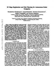
4.3 This figure illustrates the two types of errors that could be on a map because of the partial observability of the environment. Note the differences between the belief of the robot (map) and the reality (environment). . . . . . . . . .
82
4.4 Assumptions for the unobserved part of the environment using graph representation.
. . . . . . . . . . . . . . . . . . . . . . . . . . . . . . . . . . . . .
84
4.5 The two types of errors in the map are represented in a graph. . . . . . . . .
85
LIST OF FIGURES
ix
4.6 (a) If the navigation system cannot find a way to reach the goal, then (b) it will delete all obstacles in the unobserved region to prevent false obstacles. This figure illustrates this method. . . . . . . . . . . . . . . . . . . . . . . .
91
4.7 (a) If the navigation system cannot find a way to reach the goal, then (b) it will find the barrier of obstacles (green line) enclosing the goal on the map, and it will check if the barrier actually exists. This figure illustrates this method. 92 4.8 This illustrates the method of verification of the barrier. In (a) it finds only the obstacles outside the observed region via a BFS expansion; such obstacles are grey. The is delimited by dashes. In (b) the second expansion from finds the barrier (grey). In (c) it chooses the state in the barrier that minimizes () = () + ( ). These distances are marked by dashes. . .
96
4.9 This shows an example of the difference between the effective path (solid line) and the optimal path (dash line). The first is produced because initially the environment is unknown. The second is determined when the environment is known completely and correctly.
. . . . . . . . . . . . . . . . . . . . . . . .
98
4.10 The average of the path length [ ] together with an interval of one standard deviation as a function of obstacles density, when initially the environment is unknown.
. . . . . . . . . . . . . . . . . . . . . . . . . . . . . . . . . . .
99
4.11 This figure shows the probability of achieving the goal (success index) when the map has errors (dissimilarity of map), considering different densities of obstacles and knowing a map initially (KSA). . . . . . . . . . . . . . . . . . 101 4.12 This figure compares KSA (blue line) and FSA (red line) in terms of suboptimality, considering different densities of obstacles. . . . . . . . . . . . . . . 102 4.13 When the map has few errors (dissimilarity 10%), is better to verify the barrier (blue lines); and when the map has many errors (dissimilarity 10%), it is better to delete the unobserved region of the map (black lines). The red lines are obtained by using FSA from the beginning, which has the best suboptimality at high dissimilarity ( 10%). . . . . . . . . . . . . . . . . . . 103
x
LIST OF FIGURES 4.14 This illustrates the navigation in unknown environments using (a) FSA and (b) USA. The former generates paths across the whole map, even in the unobserved region, while the latter only makes plans within the observed region. This could be a computational advantage. . . . . . . . . . . . . . . . . . . . 106 4.15 The figures show the different functions to be minimized to select a partial goal at the frontier. . . . . . . . . . . . . . . . . . . . . . . . . . . . . . . . . 107 4.16 Path length [ ] to complete navigation tasks in unknown environments using FSA and USA with different cost functions.
. . . . . . . . . . . . . . 109
4.17 Average computation time to complete navigation tasks in unknown environments using FSA and USA with different cost functions. . . . . . . . . . . . 110 5.1 Erik Zamora Gómez, author of this thesis. . . . . . . . . . . . . . . . . . . . 116 6.1 We show some parameters in the model of Borenstein for odometry. . . . . . 119 6.2 Initial and final poses are marked by a circle and a cross, respectively. Note that nominal values do not obtain a good odometry.
. . . . . . . . . . . . . 120
6.3 Initial and final poses are marked by a circle and a cross, respectively. The calibrated parameters improve the accuracy of odometry.
. . . . . . . . . . 120
6.4 Red lines represent the laser beams and only the cells that passed the laser beam are updated with free or occupy probability (grey = 0.5, black = 1.0 and white = 0.0). . . . . . . . . . . . . . . . . . . . . . . . . . . . . . . . . . 122 6.5 The grid maps of second and ground floors at Automatic Control Department, Zacatenco, CINVESTAV. . . . . . . . . . . . . . . . . . . . . . . . . . . . . . 122 6.6 This is a small grid map as an example. (a) The robot can only move 8 different ways. The cost of action is assigned by Euclidean distance. (b) The value function is calculated according to the Algorithm 6.1. (c) The best action the robot can take is represented by arrows. (d) It shows two paths (blue and green) from different initial states.
. . . . . . . . . . . . . . . . . 123
LIST OF FIGURES
xi
6.7 In order to prevent the generated paths are very close to the real obstacles (a), we artificially widen the obstacles in the map according with the size of robot (b). . . . . . . . . . . . . . . . . . . . . . . . . . . . . . . . . . . . . . 125 6.8 We show the original and smooth path for comparison. . . . . . . . . . . . . 127 6.9 After the smooth process, the orientation has smooth transitions. . . . . . . 127 6.10 After the smooth process, the curvature is limited 4−1 . . . . . . . . . 128 6.11 The discrete-time controller is applied to an continuous-time unicycle model that represent the kinematics of Koala robot. The simulation considers the velocity saturation effect in left and right wheel. . . . . . . . . . . . . . . . . 130 6.12 We show how the controller follows the reference trajectories (red lines). Blue lines are robot trajectories. . . . . . . . . . . . . . . . . . . . . . . . . . . . . 131 6.13 An small autonomous navigation experiment. . . . . . . . . . . . . . . . . . 133 6.14 We show the signals that were used to guide the robot to the emergency exit. And we show some pictures of the environment in which the robot navigates and how the signals were set. . . . . . . . . . . . . . . . . . . . . . . . . . . 135 6.15 This is the diagram of the navigation system. . . . . . . . . . . . . . . . . . 136 6.16 This illustrates the matching process between templates of arrows and the image of emergency signal to recognize the direction to the emergency signal. 138 6.17 This shows (a) the region that the camera RGBD can detect obstacles and (b) the horizontal region where the shortest depth is determined. . . . . . . . 138 6.18 This illustrates how to calculate a goal ( ) through information provided by emergency signal ( ). The goal is used by A* search to compute the path, which is a sequence of points (in blue).
. . . . . . . . . . . . . . . 141
6.19 We show some snapshots during the travel of robot to the emergency exit. . 143
xii
LIST OF FIGURES
Chapter 1 Introduction "Ask not what your country can do for you; ask what you can do for your country." –John F Kennedy Why is it important to develop autonomous navigation robots? Basically, there are three kinds of robots: operated, automatic and autonomous. Operated robots are those that require control by a human, e.g. teleoperated robots for surgery or army exploration. Automatic robots do preprogrammed and repeated activities in controlled environments, e.g. robotic arms in car production lines or line follower robots. In contrast, autonomous robots do tasks in unstructured environments and make their own decisions as a function of the given goal, e.g. courier robots in hospitals and driverless cars in cities. The tendency is to give robots more autonomy, which means robots do tasks with as little human assistance as possible. Autonomous robots could catapult the productivity and quality of various human activities. Some applications are: package delivery, cleaning, agriculture, surveillance, search & rescue, building and transportation. However, a basic task that robots must do is to navigate in natural and human environments in order to achieve these applications. If someday we wish to have robots that build our highways, clean our streets, and grow and harvest our food, it is crucial they be able to navigate in unstructured environments. The mission of this thesis is to contribute to this goal: solving some problems of autonomous navigation
2
Introduction
Figure 1.1: Subsystems needed to solve the whole autonomous navigation problem. in unstructured environments. Autonomous navigation is the capacity of a robot to navigate with as little human assistance as possible. Unstructured environment is an environment that is NOT adapted to facilitate robot navigation, but is given as it is; e.g. offices, parks, streets, forests, desert, etc. Navigation in unstructured environments is a problem with many variants. The technical difficulties to be overcome to navigate depend on the type of environment: in air, on land, at sea or under the sea. The type of locomotion also ims restrictions: wheels, legs, propellers, etc. In this thesis, we limit our work to robots in terrestrial environments with flat surfaces and we use only wheeled robots. Although navigation is easy for humans, it is a difficult task for robots. Because they must navigate in unstructured environments without damage and should use several subsystems to solve the problem. Figure 1.1 shows an autonomous navigation system consisting of: • Perception: Interprets the numbers sent by sensors to recognize objects, places, and
1.1 Motivation of research
3
events that occur in the environment, or in the robot. In this way, the robot can prevent damage, know where it is, or know how the environment is. • Map building: Creates a numerical model of the environment around the robot. The map allows the robot to make appropriate decisions and avoid damage.
• Location: Estimates the robot’s position relative to the map. This helps it plan and execute movements, and build a correct map of the environment.
• Planning: Decides the movements necessary to reach the goal without colliding and in minimum time or distance.
• Control: Ensures the planned movements are executed, despite unexpected disturbances.
• Obstacle avoidance: Avoids crashing into moving objects, such as people, animals, doors, furniture or other robots that are not on the map.
The contributions of this thesis are mainly related to map building and planning because we identified relevant research opportunities, as we explain in the next section.
1.1
Motivation of research
Autonomous navigation has been developing for almost fifty years and just in the last decade has some useful results (see section 2.1). It is too large a problem to be solved with only one study. Therefore, we decided to focus on two subproblems: • Map-building problem. If we want to navigate through an environment, we need a map for two reasons: (1) to localize the robot and the goal, and (2) to plan a path between the robot’s position and the goal position. But sometimes there are no maps of buildings, public spaces or cities that can be useful for navigation. Consequently, the robot must create its own map. In unstructured environments, the map building
4
Introduction process requires knowing the robot’s position, and the robot’s position estimation requires a map. So we need to locate the robot and make the map at the same time. This is why the map-building problem is so interesting and also problematic: errors in position and map estimation affect each other, producing inconsistent maps. The effectiveness and efficiency of navigation depends on having a map without large errors. Most map building methods are based on the Gaussian assumption (i.e. estimation errors are described by a Gaussian probability distribution). But this assumption is incorrect because the real error distributions are not Gaussian. So we propose and study the Ellipsoidal SLAM method1 , which avoids the use of the Gaussian distribution. Besides, we note that other methods based on sets (i.e. estimation errors modeled by sets) cannot solve large-scale mapping problems. Our method can.
• Planning in dynamic and unknown environments. In these types of environ-
ments, the problem of partial observability is important because planning has to make certain assumptions about the environment that cannot be or has not been observed. And these assumptions might be wrong. Even if we have a perfect mapping method, the map might have errors relative to real environment. Why is this possible? The reason is simple: environments are dynamic and all sensors have a limited range of observation. This type of problem is important to solve because it affects the optimality of the path length and completeness of navigation task (i.e. to be able to reach the goal when a solution exists). We present theorems of conditions sufficient to guarantee that
a navigation system can complete its task. We propose the first methods to recover from false obstacles on the map in dynamic environments. And we propose a method to navigate more efficiently in unknown environments.
1.2 Structure of the thesis
5
Introduction Chap. 1
State‐of‐the‐art Chap. 2
Appendices Chap. 6
Autonomous Navigation Section 2.1
SLAM Section 2.2
Motion Planning Section 2.3
Navigation in dynamic and unknown environments
Ellipsiodal SLAM Chap. 3
Chap. 4
Conclusion Chap. 5
Figure 1.2: This is the general structure of the thesis.
6
Introduction
1.2
Structure of the thesis
The thesis is organized as Figure 1.2 shows. Chapter 2. We establish the state of the art of autonomous navigation (section 2.1), the map-building problem (section 2.2), and the planning problem (section 2.3). The first describes the big picture of autonomous robots, presenting the main achievements, the potential applications and the main technical problems. The second summarizes the different approaches to solve the map-building problem and shows why is important. The third explains what the planning problem is, discusses the various methods of planning and presents research work related to the problem of partial observability. Chapter 3. We propose the first map building method based on ellipsoidal sets that can solve large-scale problems. We present the method and analyze its convergence and stability by a Lyapunov-like technique. We validate the Ellipsoidal SLAM with simulations and experiments using the Victoria Park dataset and Koala mobile robot. Chapter 4. We analyze the assumptions that a robot could make in unobserved parts of the environment during navigation. We present the theorems of sufficient conditions to ensure a navigation system is complete. For dynamic environments, we propose the first methods to recover from false obstacles on the map. And for unknown environments, we propose a method to navigate more efficiently in unknown environments compared with the classical approach. We present Monte Carlo simulations to evaluate the performance of these algorithms and discuss their results. Chapter 6 (Appendices). We present the two navigation systems that were implemented during the development of doctoral research. One of them was used in the experiments for the Ellipsoidal SLAM.
1
In this thesis we consider the terms "map building" and "SLAM" synonyms, where SLAM means Sim-
ultaneous Localization And Mapping
1.3 Contributions
1.3
7
Contributions
The main contributions of this thesis are the following: • We propose the first map building method based on sets that can solve large-scale problems.
• We propose the first methods to recover from false obstacles and make the robot continue searching for the goal in dynamic environments.
• We propose a method to navigate more efficiently in unknown environments.
1.4
Products
1.4.1
Publications
We produce the following papers for publication: In journals: • Erik Zamora, Wen Yu, Recent Advances on Simultaneous Localization and Mapping (SLAM) for Mobile Robots, IETE Technical Review, 2013. (impact factor 0.925)
• Erik Zamora, Alberto Soria, Wen Yu, “Ellipsoid SLAM: A Novel Set Membership Method for Simultaneous Localization and Mapping”, Autonomous Robots, Springer (in revision). • Erik Zamora, Wen Yu, Novel Autonomous Navigation Algorithms in Dynamic and Unknown Environments, Cybernetics and Systems (in revision).
• Erik Zamora, Robots Autónomos: Navegación, Komputer Sapiens, SMIA, Enero 2015. In conferences:
8
Introduction • Erik Zamora, Wen Yu, Novel Autonomous Navigation Algorithms in Dynamic and Unknown Environments, 2014 IEEE International Conference on Systems, Man, and Cybernetics, San Diego, California, USA, October 5-8, 2014. • Erik Zamora, Wen Yu, Mobile Robot Navigation in Dynamic and Unknown Environments, 2014 IEEE Multi-conference on Systems and Control, October 8-10, 2014, Antibes, France. • Erik Zamora, Wen Yu, Ellipsoid SLAM: A Novel On-line Set Membership Method for Simultaneous Localization and Mapping, 53rd IEEE Conference on Decision and Control, Los Angeles, California, USA, December 15-17, 2014.
1.4.2
Education of human resources
As part of teaching profession, the author of this thesis collaborated in the education and graduation of 11 engineers at the UPIITA-IPN (Unidad Interdisciplinaria Profesional en Ingeniería y Tecnologáas Avanzadas del Instituto Politecnico Nacional). Four terminal works related to autonomous robotics were done (see Figure 1.3). • a) Modelado y control de un cuadrirrotor para vuelo en entornos cerrados
implementando visión artificial (Modeling and control of a quadrotor flight in closed environments by implementing computer vision). They developed a system that allows navigating a quadrotor along a corridor using only visual information from a RGB camera. Anguiano Torres Iván Adrián, Garrido Reyes Miguel Daniel, Martínez Loredo Jonathan Emmanuelle, UPIITA-IPN, 2013.
• b) Sistema de navegación evasor de obstáculos en un robot móvil (Navigation system with an obstacles avoidance for a mobile robot). This project develops a reactive
navigation system, which allows driving a mobile robot from a starting point to any point within the working area avoiding static obstacles along its path. Miguel Antonio Lagunes Fortiz, UPIITA-IPN, 2014.
1.4 Products
9
• c) Diseño, manufactura e implementación de un sistema de seguimiento de objetos mediante visión artificial para un robot humanoide NAO (Design,
manufacture and implementation of an object tracking system using artificial vision for a humanoid robot NAO). The terminal work aims to develop an embedded system for controlling movement of a humanoid, being able to locate and track an object specific color. Conde Rangel María Gisel, García Reséndiz Erick Gabriel, Serra Ramírez Jaime, Trujillo Sánchez Juan Carlos, 2013. • d) Implementación de visión artificial en un cuadrirrotor para el seguimiento de objetivos (Implementation of artificial vision in quadrotor for tracking targets).
This project involves the development of control algorithms for the flight of a quadrotor, taking into account the response of inertial sensors: accelerometer and gyroscope. In addition, it implements computer vision algorithms to follow a specific target on the ground. Hernández Espinosa Josué Israel, Montesinos Morales José Iván, Torres Vázquez Benjamín, 2012.
1.4.3
Autonomous navigation systems
During the research, we developed two autonomous navigation systems in order to put into practice some of the results of the thesis. Here we briefly present these systems, and we describe them in detail in the appendices of thesis. 1. A basic autonomous navigation system. At the beginning of the PhD program, it was necessary to develop an autonomous navigation system for robot Koala; in order to carry out experiments of the SLAM method proposed in this thesis. This robot is available in the laboratory of the Department of Automatic Control. The navigation system is comprised of four subsystems: localization, mapping, planning and controller. The localization is done by odometry that integrates the angular displacements of encoders. The mapping builds a 2-D occupancy grid map using odometry and information from a laser. The planning is conducted by the method of dynamic
10
Introduction
Figure 1.3: We show some snapshots of terminal projects and engineers that the author of this thesis has instructed in UPIITA-IPN during the development of his PhD research (see text for more details).
1.4 Products
11
programming with a smoothing method for the generated path. The control is carried out by a nonlinear controller which follows the smoothed path. The software was written in Python and C/C++. This navigation system is very basic because it does not use a SLAM technique to correct the odometry errors on map. Therefore, this system cannot be used to navigate distances greater than 20 meters. However, it was useful for our experiments. Figure 1.4 shows how the robot navigates through a door along the planned path. 2. Navigation in unknown environments guided by emergency signs. As part of the PhD program, the author of this thesis participated in a research stay at the University of Bristol in England led by Walterio Mayol-Cuevas. The aim of the research stay was to develop a navigation system for a differential mobile robot (iRobot). The task was to look for the emergency exit guided by the existing emergency signs on the building. Figure 1.5 shows some examples of these emergency signs and the robot moving to the exit. The robot uses a RGBD camera (Kinect) to detect emergency signs and determine the direction that it should move. The same sensor provides information on obstacles such as chairs, walls, tables, people, etc. It uses a SLAM method (Gmapping method) to build a 2-D map as it moves; at the beginning the robot does not know the environment. It uses a planning method (A* search) to find the shortest path. This method was modified to integrate the information of emergency signs. The planned path is executed by a P controller and a method of obstacle avoidance (Smooth Nearness Diagram) was added. All software is written in Python and C/C++ on ROS platform (Robot Operating System). The most interesting part of this project was to implement the system of perception which must detect, recognize and interpret the emergency signs to know how to move. Furthermore, it was necessary to implement a system to prevent repeated detections which was coupled to the SLAM method. A video showing the operation of this navigation system is online at https://www.youtube.com/watch?v=RAj70AGsXls&feature=youtu.be??
12
Introduction
Figure 1.4: We show how the Koala robot can navigate through a door along the planned path using a map that was previously built. The map was constructed while controlling the robot manually.
1.4 Products
13
Figure 1.5: We show a snapshot of the robot reaching its goal: the emergency exit. We also show the emergency signs in the building in the University of Bristol. They were used to guide the robot to its goal.
14
Introduction
Chapter 2 State of the art The aim of this chapter is to show an overview of autonomous navigation, the map-building problem, and the planning problem. This chapter is divided into three main sections. The first describes the big picture of autonomous robots presenting the main achievements, the potential applications, and the main technical problems. The second summarizes the different approaches to solve the map-building problem and show why it is important. The third explains what the planning problem is, discusses the various methods of planning, and presents research work related to the problem of partial observability.
2.1
Autonomous navigation "The world requires practical dreamers who can, and will, put their dreams into action." –Napoleon Hill
Why is it important to develop autonomous navigation? Basically, there are three kinds of robots: operated, automatic, and autonomous. Operated robots are those that require control by humans (e.g., teleoperated robots for surgery or army exploration). Automatic robots do preprogrammed and repeated activities in controlled environments (e.g., robotic arms in car production lines or line follower robots). In contrast, autonomous robots do tasks in natural and unstructured environments and make their own decisions as a function
16
State of the art
of the given task goal (e.g., courier robots in hospitals and driverless cars in cities). The tendency is to give robots more autonomy, which means robots do tasks with as little human assistance as possible. A basic task that robots must do is to navigate in natural and human environments. If someday we wish to have robots that build our buildings and highways, clean our streets, grow and harvest our food, it is crucial they are able to navigate in unstructured environments. There have been incremental advancements in the last 15 years. In the following three subsections, we will revise some breakthroughs, mention some of the applications for autonomous robots and describe what the main problems are, respectively.
2.1.1
Breakthroughs and companies
In 2004 and 2005, several vehicles navigated autonomously through the Mojave Desert, travelling about 200 km, following a map of GPS coordinates and using a set of lasers and cameras to avoid the obstacles on the route. The robotic vehicles were built by universities and companies, and the driverless car challenge was organized by DARPA (Defense Advanced Research Projects Agency in the USA). In 2007, there was another competition, but in an urban environment, which is a harder challenge. The vehicles had to avoid crashing into cars, bikes, and pavement; to execute driving skills such as lane changes, U-turns, parking, and merging into moving traffic. The winners for the 2005 and 2007 challenges were Stanley [1] from Stanford University and Boss [2] from Carnegie Mellon University; you can see these vehicles in Figure 2.1. Based on these results, Google Inc. has developed several autonomous cars that have been tested in cities and highways, in Nevada and California, USA, where the government already gives restricted driver license for autonomous cars. A disadvantage of Google cars is its high cost because of the 3-D sensor (Velodyne costs about $75,000) and high-precision GPS. Thus, the University of Oxford has launched the project RobotCar UK to replace this expensive sensor with cheaper lasers and cameras, using the spatial-visual information to localize the robot without GPS [3].
2.1 Autonomous navigation
17
Figure 2.1: Some autonomous cars are able to navigate in deserts, cities, and highways: (a) Stanley, (b) Boss, (c) Google driverless car, (d) RobotCar UK.
18
State of the art Humanoid robots (see Figure 2.2) will evolve toward autonomy, but currently they show
limited capabilities. Asimo has automatic skills, including jumping with only one foot, running, climbing stairs, opening bottles, pouring liquids from one glass to another. However, most activities are preprogrammed by humans and are not autonomous, so they cannot find and execute the suitable motions to solve the task by themselves. Other humanoids like Atlas, Justin, Reem, Charli or HRP-4C suffer from the same problem. But there are advancements in motion planning, learning, and perception to give them more autonomy. Some examples are the algorithms tested in PR2 [4] and iCub [5]; they can decide how to move their arms to grasp bottles without hitting the table or other objects. Due to the nuclear disaster in Fukushima, DARPA is organizing another competition, Darpa Robotics Challenge [6]. The goal is to develop algorithms that make humanoids assist humans in natural and man-made disasters. This challenge will bring new technologies to catapult forward development of autonomous robots. Several autonomous robots exist in Mexico: Justina [7], Golem [8], Markovito [9], Donaxi [10] and Mex-One (see Figure 2.3). The first four can navigate autonomously indoors, moving toward previously visited places and avoiding obstacles. They can do some tasks, like recognizing objects, people, and voice; cleaning tables; grasping bottles; speaking some preprogrammed sentences. These robots have competed in Robocup@home, which is a competition of service robotics, where Golem won the prize for innovation in 2013. On the other hand, Mex-One will be the first Mexican biped robot, but it is still in development. It promises to be a great platform to test algorithms to transform it into an autonomous robot. Besides, there are Mexican robots that compete in RoboCup@Soccer and RoboCup Rescue; some of them do autonomous tasks, like play football or build a map inside a collapsed building. Several companies produce autonomous robots. In the United States, three companies target infant industry (see Figure 2.4). Boston Dynamics has made a reputation with its impressive robotic mules able to travel on rough terrain. Willow Garage produces PR2, which has been tested if it can fold laundry or play billiards. But his most important contribution is continuing the development of the operating system for robots ROS (Robot Operating
2.1 Autonomous navigation
19
Figure 2.2: We show some humanoid robots useful for researching motion planning, perception, and learning algorithms, with the objective of giving them autonomy.
20
State of the art
Figure 2.3: Mexican autonomous robots
System), whose license is free and supports a considerable number of commercial robots. Rethink Robotics sells Baxter, a manufacturing robot that does not require a specialist to code tasks since anyone can program it with a friendly graphical interface and moving robot arms to indicate the task. Moreover, in Germany, BlueBotics produces and sells mobile robots with autonomous navigation systems, guiding tourists in cities and museums. These are some examples of how the robotics industry moves toward autonomy. The industry for autonomous robots is almost nil in Mexico. This is a great opportunity for investors and entrepreneurs since the market is virgin, waiting for someone to exploit it. The company, called 3D Robotics, has done this; it was cofounded by a Mexican and an American, and it produces and distributes unmanned aerial vehicles with a navigation system based on GPS. The rest of the Mexican industry sells robots and accessories, gives courses, and installs automatic robots for manufacturing.
2.1 Autonomous navigation
21
Figure 2.4: Companies of autonomous robots.
2.1.2
Applications
Autonomous robots catapult the productivity and quality of various human activities. Here we will present some existing applications and imagine other possibilities. • Package delivery. Imagine a robotic motorcycle or quadcopter that delivers pizza to your front door. In the near future, companies will begin to send small packages
with fast food, bills, documents, books, or DVDs using autonomous robots. One advantage is that the flying vehicles can take the sky, unlike human messengers. In 2013, Amazon announced that it is willing to test this idea, creating a new delivery system to get packages into customers’ hands using drones [11]. The Matternet project [12] proposes quadcopters forming a network to distribute food and medicine. There are already robotic messengers carrying medicine and documents between departments in hospitals [13] (see Figure 2.5). • Cleaning. Cleanliness and order are important in any advanced civilization. But
22
State of the art cleaning and maintaining order have always been heavy and monotonous activities. Robots can perform these tasks for us at home and in public places. Take a look at the current progress: iRoomba cleans the floors of homes [14], Lely Discovery keeps the environment of cows hygienic at farms [15], and Ambrogio maintains lawn at the desired height in your garden [16]. This is just the beginning. • Agriculture. The machinery added in the 20th century has allowed modern agricul-
ture to increase its productivity and to free humans to do other activities that develop civilization. The company John Deere estimates that 90% of the U.S. population in 1848 was involved in agriculture, and today it is about 0.9%, partly because of the machinery for harvesting and planting. Why not automate it? The algorithms developed for autonomous navigation may allow the machinery to produce the same with minimal human intervention and supervision for repairs. See these references: in Australia [17][18] and Denmark [19], people are giving autonomy to agricultural machinery. In some years, we will see companies exploiting these opportunities; I wish they are Mexican.
• Surveillance. Algorithms to perceive and model the environment might be used to
monitor human behavior. Imagine quadcopters looking for criminals on the streets and reporting it to the nearest police officer. Imagine watchdog robots at home that detect the entry of an unknown person or when a window breaks. The Japanese company Secom has developed two autonomous robots for surveillance and promises to put them on the market [20].
• Search and Rescue. In Mexico, one of the basic tasks of Plan DN-III-E is to search and rescue in disasters. The Mexican army could use mobile robots to find people trapped in dangerous places. With the information you collect, the robot can serve to create a better bailout. Currently, most robots are teleoperated [21]. But giving them the ability to navigate and search, a group of robots can cover the same area faster, increasing the likelihood of rescuing people. Search and rescue have several challenges: mobility on land with debris, enough power for long missions, identifying victims,
2.1 Autonomous navigation
23
Package Delivery
Cleaning
Agriculture
Surveillance
Figure 2.5: Package delivery: quadcopter and station to provide food and medicines to rural areas; RobotCourier to transport substances and documents in hospitals. Cleaning: iRoomba autonomous vacuum cleaner; Ambrogio, autonomous mower; Lely Discovery, cleaner for farms. Agriculture: autonomous agricultural machinery. Surveillance: Secom company’s robots.
24
State of the art and others. The RoboCupRescue competition aims to overcome these limitations (see Figure 2.6). A team who took part in this competition, the Hector Team Darmstadt [22], has developed robots with search and rescue skills, including map building in not planar floors, detecting victims, planning motion, semantic mapping, etc.
• Building. The construction industry can benefit from robotics as the manufacturing
industry has done. Robots would liberate humans from heavy labor, improving their life quality. A city could build people’s homes faster and cheaper. Although construction robotics is emerging, there is some progress: space exploration robots carry metal bars to form walls [23], quadcopters build cubic structures [24], and mobile robots with mechanical arms build furniture [25].
• Transportation. Most goods you use were brought from distant places; this is pos-
sible by planes, cars, and boats which amplify human force. In the future, we will see those vehicles moving with minimal human assistance, increasing productivity, efficiency, and safety (reducing the number of accidents). Cities will have autonomous public transport (e.g., there was a demonstration of an autonomous minibus in the Intelligent Vehicles Symposium 2012). Also, short-distance transportation can benefit: Kiva company sells a robotic system that handles the inputs and outputs of a warehouse [26].
• Guiding People. Since 1997, there have been robots that interact with visitors in
museums [27][28], explain the exhibits, and guide people. This technology can also be used in guiding blind people or for advertising in malls, football stadiums, and concerts. Imagine a sales robot that is appealing to the public and engages people to offer them a product. Imagine flying robots that align to form shapes in the air while they advertise a service.
2.1 Autonomous navigation
25
Search and Rescue
Building
Transportation
Guiding People
Figure 2.6: Search and Rescue: Japanese robot to retrieve people; maritime quadcopter to monitor seas; robot to find people in collapsed buildings. Building: rovers stacking rods; quadcopters building cubic structures; mobile robots building a small table. Transportation: a minibus navigates autonomously; the Kika robot system that handles the inputs and outputs of a warehouse. Guiding People: Rhino, one of the first robots that guides visitors in a museum; a more current guide robot; robotic dog for blind people.
26
State of the art
2.1.3
Main problems
Each of the above applications has specific challenges, but they share autonomous navigation as a problem. Even though navigation is easy for humans, it is a difficult task for robots. They must navigate in unstructured environments, reaching the given target without damage. To achieve this goal, the robot should solve different subproblems. Figure 2.7 shows a system of autonomous navigation. The body of the robot has the following: • Sensors send pieces of information about the environment and the robot’s state (e.g., distance to the nearest object or robot speed).
• Actuators execute the motions that the computer commands (e.g., electric motors). The robot’s mind is a set of algorithms executed by the computer: • Perception: Interprets the numbers sent by the sensors to recognize objects, places,
and events that occur in the environment or in the robot. In this way, the robot can prevent damage, know where it is, or know how the environment is.
• Map building: Creates a numerical model of the environment around the robot. This allows the robot to make appropriate decisions and avoid damage.
• Location: Estimates the robot’s position with respect to the map. This helps it plan and execute movements, and build a correct map of the environment.
• Planning: Decides the movements necessary to reach the goal without colliding and in minimum time or distance.
• Control: Ensures the planned movements are executed, despite unexpected disturbances.
• Obstacle avoidance: Avoids crashing into moving objects, such as people, animals, doors, furniture, or other robots that are not on the map.
2.1 Autonomous navigation
27
Figure 2.7: This illustrates the subsystems needed to solve the whole autonomous navigation problem.
28
State of the art Algorithms already exist for each of these tasks [29]. The problem of navigation in unstructured environments presents several challenges.
However, this thesis only focuses on two specific problems. 1. Map building (SLAM, Simultaneous Localization and Mapping). The effectiveness and efficiency of navigation depends on having a map with no errors. Most map-building methods are based on the Gaussian assumption (i.e., estimation errors modeled by a Gaussian probability distribution). But this assumption is incorrect because the real error distributions are not Gaussian. So we propose and study a new method that avoids the use of the Gaussian distribution, and errors are modeled by ellipsoidal sets. Besides, none of the other methods based on sets has shown to be able to build large-scale maps. Our method can. 2. Planning in dynamic and unknown environments. In these types of environments, the problem of partial observability is important because planning has to make certain assumptions about the environment that cannot be or has not been observed. And these assumptions may be wrong. Even if we have a perfect mapping method, the map might have errors relative to the real environment. This type of problem is important to solve because it affects the optimality of the path length and the completeness of the navigation task (i.e., to be able to reach the goal when a solution exists). We present theorems of sufficient conditions to guarantee that a navigation system can complete its task. We propose the first methods to recover from false obstacles on the map in dynamic environments. And we propose a method to navigate more efficiently in unknown environments. In the next two sections, we present the state of the art of these two problems: map building and planning. And we give more details on these issues.
2.2
SLAM "It is only by learning from mistakes that progress is made." –Sir James Dyson
2.2 SLAM
2.2.1
29
SLAM problem
The objective of simultaneous localization and mapping (SLAM) is to build a map and to locate the robot in that map at the same time. We should clarify that for the SLAM problem, it does not matter if the robot moves autonomously or is controlled by a human. The important thing is to build the map and locate the robot correctly. The most basic way to locate a robot is using odometry. For a terrestrial mobile robot, odometry consists of integrating the displacements measured by encoders to estimate the position and orientation of the robot. The problem is that odometer error accumulates as the robot moves. Eventually, the error is so large that odometry no longer gives a good estimate of the state of the robot, as shown in Figure 2.8. Then the robot must make observations of some references in the environment to correct the odometer error, assuming the references are static. When the robot returns to observe, these references can reduce the accumulated error. The main work of the SLAM method is to correct the estimation of the robot state and the map. On the other hand, the SLAM is a chicken-and-egg problem because the robot needs a map to locate itself and the map needs the localization of the robot to build a consistent map. Thus SLAM methods must be recursive. This is why the SLAM problem is so difficult because errors in robot and map states affect each other, producing inconsistent maps. In the following section, we will give an overview of several SLAM methods.
2.2.2
SLAM solutions
In the last decade, many types of SLAM have been developed. They can be categorized by different criteria, such as state estimation techniques, type of map, real-time performance, the sensors, etc. However, we classify the techniques according to the type of problem they solve into the following four categories: Feature-based SLAM, Pose-based SLAM, Appearancebased SLAM, and Other SLAMs. In Figure 2.9, we compare these main SLAM paradigms. Feature-based SLAM. Odometer error can be corrected by the use of landmarks in the environment as references. Consider a mobile robot that moves through an environment,
30
State of the art
Odometry Observations
SLAM Method
Robot state Map
Objective: Reduce errors Figure 2.8: The goal of the SLAM method is to build a consistent map and locate the robot during its journey. In general, SLAM methods integrate the observations of some references in the environment with the odometry to reduce errors.
2.2 SLAM
31
Figure 2.9: We compare the main SLAM paradigms in terms of their capacity to solve some problems and the type of map they build. Loop-closure performance measures the ability to close the loop when the robot revisits the same place. The wake-up robot problem, also called global localization, refers to a situation where a robot is carried to an arbitrary location and put to operation; the robot must localize itself without any prior knowledge. The kidnapped robot problem refers to a situation where a robot in operation is carried to an arbitrary location; the robot must localize itself, avoiding confusions.
32
State of the art
z1k-1
z1k+2
z2k-1 z3k-1
uk-2 xk-2
z4k-1
z2k+1 z1 k
uk-1 xk-1 z2k
z1k+1
uk+1
uk xk
xk+1
z3k+1
Figure 2.10: The robot simultaneously builds a map and localizes itself. At each time step , the robot moves according to controls u−1 and takes some observations z = {z z }
at the pose x .
as represented in Figure 2.10. In the beginning, we can take the initial robot position as zero. The robot must be able to detect some specific objects in the environments, which are called landmarks. This robot must also be able to measure the distance between its position x and landmark positions m in the environment and also measure the angle between the robot-landmark line and some reference line. At each time step , the robot moves according to controls u−1 and takes measurements z = {z z } at the state x . There are three tasks shown in Figure 2.11 that any feature-based SLAM method must do. (1) Landmark detection. The robot must recognize some specific objects in the environment; they are called landmarks. It is common to use a laser range finder or cameras to recognize landmarks, such as corners, lines, trees, etc. (2) Data association. Detected landmarks should be associated with the landmarks on the map. Because landmarks are not distinguishable, the association may be wrong, causing large errors on the map. Besides, the number of possible associations can grow exponentially over time; therefore, data association
2.2 SLAM
S e n s o r s
33
Odometry
Landmarks Detection
Data Association
State Estimation
Robot state Map
Observations
Figure 2.11: Any method of feature-based SLAM must do these tasks: detecting landmarks on the environment, associating the detected landmarks with the landmarks on the map, and improving the estimate of the robot’s position and the map. is a difficult task. (3) State estimation. It takes observations and odometry to reduce errors. The convergence, accuracy, and consistency of the state estimation are the most important properties. In this thesis, we focus on state estimation task. The major difficulties of any SLAM method are the following: • High dimensionality. Since the map dimension always grows when the robot explores the environment, the memory requirements and time processing of the state estim-
ation increase. Some submapping techniques can be used to solve it (metric-metric approaches [52][53][54], topological-metric approaches [55][56][57]). • Loop closure. When the robot revisits a past place, the accumulated odometry error
might be large. Then the data association and landmark detection must be effective to correct the odometry. Place recognition techniques are used to cope with the loop closure problem [71][78].
• Dynamics in environment. State estimation and data association can be confused by the inconsistent measurements in the dynamic environment. There are some methods that try to deal with these environments [36][85][86][87].
34
State of the art Pose-based SLAM. It estimates only the robot’s state. It is easier than feature-based
SLAM because the landmark positions are not estimated. However, it must maintain the robot path, and it uses the landmarks to extract metric constraints to compensate the odometer error. Therefore, the high dimensionality limitation arises from the dimension growing by robot states rather than by the landmark states. Landmark detection, data association, loop closure, and dynamic environment still are relevant problems. Most posebased SLAMs employ a laser range finder and the laser scans that form the occupancy grid maps of the environment (if the odometry is corrected, the grid map is right). Instead of using the landmark detector, the laser scan transforms the data association problem as an matching of laser scans for extracting the constraints. This problem is also called front-end problem and is typically hard due to potential ambiguities or symmetries in the environment. Path estimation can be performed by optimization techniques [33][62][63][64][65][66] [67][68], information filters [34][69], and particle filters [70][35]. Appearance-based SLAM. It does not use metric information. The robot path is not tracked in a metric sense; instead, it estimates a topological map of places. Topological maps are useful for global motion planning, but not for obstacles avoidance. The configurations of the landmarks of a given place can be used to recognize the place; visual images or spatial information are also utilized to recognize the place. The metric estimation problem is avoided, but data association is still an important problem to solve. Loop closure is performed in the topological space. High dimensionality is translated into the number of places in the topological map. It is very common that these appearance techniques are used complementary to any metric SLAM method to detect loop closures [36]. Some methods based on visual appearance are [71][72][73][74][75][76][77][78], and others based on spatial appearance are [79][80]. Other SLAMs. There are several variants of the SLAM problem that cannot be included in the above paradigms. Pedestrian SLAM employs light and cheap sensors and faces the obstacle of human movements, which are different to robot behavior [37][81][82][83]. SLAM with enriched maps uses auxiliary information on the map [38][84], such as temperature, terrain characteristics, and information form humans. Active SLAM derives a control
2.2 SLAM
35
law for robot navigation in order to efficiently achieve a certain desired accuracy of the robot location and the map [39]. Multirobot SLAM uses many robots for large environments [40]. SLAM in dynamic environments [85][86][87] deals with moving objects and agents. In this thesis, we are interested in the feature-based SLAM paradigm because it is the original form of the SLAM problem. The SLAM method we are proposing in this thesis belongs to this category. So we go into more detail about the methods to solve feature-based SLAM problems. There are two versions for feature-based SLAM [41][42]: (1) Full SLAM. It estimates the current and the past states {1 −1 } in order to know the complete robot trajectory and to estimate the landmark’s positions = {1 2 } at each time step (this is a
smoothing problem). (2) Online SLAM. It estimates only the current robot state and the landmark’s positions at each time step (this is a filtering problem). Our method (Ellipsoidal SLAM) is an Online SLAM. An important point is that there are two ways of error modeling: by probability distributions or by sets that bound the error. Our method (Ellipsoidal SLAM) uses ellipsoidal sets to model the error. In the following sections, we present the main approaches for these categories and discuss some of their limitations. Probabilistic approaches In these methods, the odometer error, the sensors’ error, and the modeling error (for example, linearization) are modeled by probability distributions. We will present an overview of the main probabilistic methods used in the SLAM problem. In Figure 2.12, we show a general comparison among them. Kalman-based SLAM. Extended Kalman Filter SLAM (EKF-SLAM) is the first solution for the Online SLAM problem, and it is the most popular method. The complete discussion can be found in [30]. Since the Gaussian noise assumption is not realistic and causes fake landmarks on the map, EKF-SLAM requires additional techniques to manage the map to eliminate the fake landmarks. The consistency and convergence of the EKF-SLAM algorithm are studied in [43], and various techniques are reviewed to overcome the incon-
36
State of the art
Figure 2.12: We compare the probabilistic methods used for feature-based SLAM problem. Note that all are assuming Gaussianity. Full SLAM estimates the complete trajectory of robot and the landmark’s positions at each time step (this is a smoothing problem). Online SLAM estimates only the current robot pose and the landmark’s positions m at each time step (this is a filtering problem).
2.2 SLAM
37
sistency problem of EKF-SLAM in [44]. The biggest disadvantage of EKF-SLAM is that its computing time is quadratic over the number of landmarks due to the update of the covariance matrix. There are several ways to overcome this limitation: (1) limiting the number of landmarks to be estimated [31], (2) updating only the part of currently detected landmarks and postponing the complete update to a later time [45], and (3) making approximations in the covariance update stage [46]. Information-based SLAM. Motivated by reducing the computing time of EKF-SLAM in larger environments, the Extended Information Filter (EIF) was developed. The great advantage of EIF over EKF is that the computing time can be reduced due to the sparseness property of the information matrix. However, the recovery of the landmark positions and the covariance associated with the landmarks in the vicinity of the robot are needed for data association, map update, and robot localization. When the number of landmarks is small, it can be obtained by the inverse of the information matrix, but the computational cost of the inversion will be unacceptable with a large information matrix. Some methods that use the information filter are: Sparse Extended Information Filter [47], Exactly Sparse Extended Information Filter [48], and Decoupled SLAM [49]. Particles-based SLAM. Particle filter is a sequential Monte Carlo inference method that approximates the exact probability distribution through a set of state samples. Its advantage is that it can represent any multi-modal probability distribution. It does not need Gaussian assumption. Its main drawback is that the sampling in a high-dimensional space is computational inefficient. But if the problem estimation has "nice structure," we can reduce the size of the space using the Rao-Blackwellized Particle Filter (RBPF), which marginalizes out some of the random variables. The RBPF is used in conjunction with the Kalman filters to estimate the positions of the landmarks (one Kalman filter for each landmark). Some methods that use particle filter are: the FastSLAM algorithm [58] and its improved versions (the UFastSLAM algorithm [59] and the Gaussian mixture probability hypothesis density (PHD) filter [60]). Graph-based SLAM. These methods use optimization techniques to transform the SLAM problem into a quadratic programming problem. The historical development of this
38
State of the art
paradigm has been focused on pose-only approaches and using the landmark positions to obtain constraints for the robot path. The objective function to optimize is obtained assuming Gaussianity. Some methods are: GraphSLAM [32], Square Root SLAM [50], and Sliding Window Filter [61]. Their main disadvantage is the high computational time they take to solve the problem. So they are suitable to build maps off-line. They are used because they are more accurate. Set-membership approaches Another way to model the error is by sets. The literature reports a few SLAM solutions using sets. Di Marco et al. [124] have developed an online algorithm. They obtain linear time complexity () with respect to the number of landmarks by state decomposition and approximating the sets as aligned boxes. The correlation between robot states and landmark positions is lost due to the decomposition state. These correlations are crucial to build a consistent map, especially when the robot closes a loop [118]; this is why we think this method is not able to solve large-scale SLAM problems. Our method (Ellipsoidal SLAM) saves these correlations as Kalman filter does. CuikSLAM [88] is a project based on interval analysis. They interpret the SLAM problem as a set of kinematic equations that are solved by interval arithmetic. Unfortunately, this work assumed that the association problem is solved and only present a simulation of a simple example to validate the algorithm. Jaulin [122][123] represents the uncertainty with intervals of real numbers. It translates the range-only and full SLAM problems in terms of a constraint satisfaction problem. It uses interval analysis and contraction techniques to find the minimal envelope of robot trajectory and the minimal sets to enclose the landmarks. This method has some limitations. It lacks the association among landmarks and observations. In [122], it requires a human operator to make the association. The algorithms must work off-line due to the large computational cost of contraction. Besides, their operation is sensitive to outliers, yielding empty sets and stopping the estimation. These shortcomings mean it can not solve large-scale SLAM
2.3 Motion planning
39
problems. In contrast, our method can deal with the association problem without a human operator, and it has the potential to work online. And more importantly, we show that it is able to build large-scale maps.
2.2.3
Conclusion
In this section, we gave an overview of the SLAM problem and its solutions. We showed that the simplest way to model the error is with a Gaussian distribution. Most methods consider Gaussianity because we only require two parameters: mean and variance. However, we know that Gaussianity is not a realistic assumption, as we will show in the next chapter. In this thesis, we are looking for a method that does not assume this. And we note that none of the SLAM methods based on sets can solve large-scale problems (with high dimensionality in the state vector). This thesis proposes a method based on ellipsoidal sets (Chapter 3). The ellipsoid filter is similar to Kalman filter, and then we can extrapolate many techniques of EKF SLAM to deal with large environments, data association, and map management.
2.3
Motion planning "The definition of insanity is doing the same thing over and over again and expecting different results." –Albert Einstein
2.3.1
Planning problem
Motion planning decides what and how to move. It has the purpose of generating a trajectory (path) in state space to reach the goal, given an environment model (map), the current state of the robot, and a goal state (see Figure 2.13). It must avoid the obstacles in the environment and must take into account the kinematic and dynamic constraints of the robot and its size. Motion planning is a difficult task because the algorithms should search for a solution on a continuous and high-dimensional state space. They must discretize the state space to make decisions as soon as possible.
40
State of the art
Robot state Map Goal state
Motion Planning Method
Trajectory of robot's state
Objective: Make motion decisions and avoid damage Figure 2.13: The motion planning method must generate a state trajectory (blue line), avoiding damage to the robot (red triangle) and reaching the goal state (G).
2.3 Motion planning
41
The motion planning problem can be stated as follows: given an environment model (an occupancy grid map, in our case), an initial state x , and a goal state x , the planning algorithm must calculate automatically a sequence of states x1 = x x2 x = x , which conforms to a free-collision trajectory, with minimal length and enough smooth, and satisfies the kinematic and dynamic constraints of the robot.
2.3.2
Planning approaches
In general, there are two kinds of planners: Graph Search, where the trajectory is searching in a graph of nodes that discretely represent the state space of the robot; and Controllers, where instead of obtaining a path, they determine the control policy for every location in the state space. We briefly review the most important algorithms for each category. A detailed explanation about the following algorithms can be found in [99][29]. Graph Search algorithms discretize the state space by creating a graph [141][142][143] with nodes that represent robot states and edges that represent the robot actions. The graph formation can be too simple, like dividing the physical space into a grid [144], or more complicated, like randomly sampling the state space [145][146]. The most common Graph Search algorithms are the following: • Breadth-First Search [100]. The nodes are explored in order of proximity. Proximity is defined as the shortest number of edge transitions. The generated path could be
the minimum-cost path (i.e., it is the optimal path) if the cost of edges is a nondecreasing function of the depth of the node. Its large disadvantage is that the memory requirement is bigger as the depth of the graph increases. • Depth-First Search [100]. In contrast to the previous algorithm, this explores each node
up to the deepest level of the graph. The advantage is that its memory requirement is less than Breadth-First Search because it stores only a single path during execution. However, this search does not guarantee finding the optimal solution.
• A* search [101][102]. It is an improvement of Dijkstra’s algorithm [103], adding a
42
State of the art heuristic function that encodes knowledge about the cost for reaching the goal. The optimal solution is guaranteed, if the heuristic is always an underestimated the cost. This heuristic reduces the number of node explorations with respect to Breadth- and Depth-First. Its main drawback is the high memory requirement because it keeps all generated nodes in memory. Some ways to face this difficulty is applying an Iterative Deepening strategy (IDA*) [100], Recursive Best-First Search (RBFS) [104], or Memory Bounded (MA* or simplified MA*) [105]. • D* algorithm [106](or D*Lite [107]). They are incremental replanning versions of A*,
where the algorithm reuses the previous search efforts, instead of generating a new solution from scratch. Search time may decrease by one or two orders of magnitude. Replanning is important in dynamic environments or when the map is corrupted by noise or when the environment is unknown.
• Anytime planners A*[108] or D*[109]. The anytime planners are suitable when the
planning time is limited. They find a feasible solution quickly (a suboptimal solution) and then continue to work on improving it until time runs out.
• Distance-propagating dynamic system [110][111]. Each node stores a current estimate of the distance to the nearest target and the neighbor node from which this distance
was determined. The update of the distance estimate at each node is done using only the information gathered from the node’s neighbors. The path is determined from the information at the robot’s current location. This algorithm can deal with dynamic obstacles or dynamic goals. • Higher geometry maze routing algorithm [112]. This algorithm is inspired by Lee’s
routing algorithm [113] in the grid plane. It can deal with any shape of robot to avoid obstacles.
• Sampling-based planners. All previous search algorithms are deterministic. In contrast, sampling-based planners are stochastic to solve complex high-dimensional motion problems for fly vehicles, humanoids, or robot manipulators in cluttered environments or
2.3 Motion planning
43
narrow passages. Some examples are Probabilistic Roadmap Planner [145], ExpansiveSpaces Tree Planner [114], and Rapidly Exploring Random Trees (RRTs) [115]. The most important Controllers are the following: • Potential field planning [93]. It is not a formal controller, but its output is a control
policy of robot direction. It creates a gradient (a virtual force) across the map that
directs the robot to the goal. This gradient is calculated by a function that continuously represents the occupied and free space of the map. The goal position is represented by the minimum of the function (attractive force), and obstacles are related to high values of the function (repulsive forces). Its main drawback is that the generated function can have local minimums depending on the shape of the obstacles (e.g., if the obstacles are concave, the robot could oscillate). To overcome this limitation, we can use the harmonic potential field method [94], which numerically solves a Laplace equation. • Dynamic programming [96]. It is a numerical method to solve optimal control problems
based on the principle of optimality developed by R. E. Bellman [95]. This method is used to generate control policy over the free space of the map. The main disadvantage is its high computational cost.
• Value Iteration [97]. It is a Markov decision process to determine a control policy,
considering the uncertainty of robot actions. Value iteration recursively calculates the utility of each action relative to a payoff function. Its drawback is also its high computational cost.
• Model Predictive Control (MPC). It uses a reference model to predict the dynamic behavior of the robot in next time step, and using an optimization technique, it de-
termines the best action controls. Tahirovic et al. [98] have studied the use of MPC with passivity-based control and a potential field representation of the environment to propose a navigation planner. Planning is performed by A* search method in this thesis because we consider that the mobile robot only moves in a plane, to simplify the problem.
44
State of the art
The effect of partial observability of environment on planning In this thesis, we are interested in studying the effect of partial observability of the environment on planning. Planning requires making some assumptions about the environment that cannot be or has not been observed to generate paths in these regions in order to reach its goal. The problem is that these assumptions about the environment may be wrong, and can cause the planning to make bad decisions. This problem is more important when environments are dynamic or unknown because there is no way to guarantee that the map and the environment are the same. Most navigation systems reported in literature [147][78][148][142] assumes to know the environment without errors or changes. Or when the environment is previously unknown, it assumes the environment is free of obstacles [148][142][149]. There have been few studies on these assumptions even though they are fundamental for the navigation problem. The assumption of free obstacles is studied in [153][150]. The aim of the authors is to analyze how suboptimal the path length is when the environment is initially unknown, focusing on the worst path length obtained by three planning methods Greedy Mappingg (GM), Dynamic A* (D*), and Chronological Backtracking (CBack). For the first two methods, the | authors derived upper (| |32 ) and lower Ω( loglog| | |) bounds on the worst-case path log| |
length as a function of the number of vertices of the graph. And the same authors showed that GM and D* can present shorter path lengths than CBack for an average-case analysis. They assume that the known area of the map is identical to the environment, which is not true, especially when the environment is dynamic. In this thesis, we study what could happen in this case, showing that it is necessary to develop algorithms to recover from map errors. This problem has been ignored systematically in literature, with the thinking that the map is always equal to the environment.
2.3.3
Conclusion
In this section, we gave an overview of the planning problem and its solutions. Besides, we showed the few papers that have addressed the problem of partial observability of the
2.3 Motion planning
45
environment and its effects on planning. Inspired by this situation, this thesis studies how this partial observability affects navigation (Chapter 4), given formal definitions for the autonomous navigation problem. We present theorems of sufficient conditions to ensure a navigation system is complete. We propose the first methods to recover from false obstacles on the map in dynamic environments. And we propose a method to navigate more efficiently in unknown environments.
46
State of the art
Chapter 3 Ellipsoidal SLAM "I have not failed. I’ve just found 10,000 ways that won’t work." –Edison
3.1
Introduction
Robotics science aims to build autonomous robots. One part of the problem consists of giving them autonomy for navigation. This implies, among other things, robots must build an environment model (i.e., a map). This problem is known as Simultaneous Localization and Mapping (SLAM) [118]: the robot must estimate the position of some landmarks in the environment and use them to estimate its state, and vice versa, use its state to estimate the landmark positions. Thus SLAM solutions are recursive. In the last 15 years, many types of SLAM methods have been developed. They can be categorized as feature-based SLAM [47], pose-based SLAM [33], and appearance-based SLAM [36]. For a more complete revision of categories and techniques, we invite the reader to consult our review [119]. In this chapter, we focus on the feature-based SLAM problem. There are some uncertainties in determining the robot’s position and the landmarks’ positions due to sensor and model errors. To compensate these errors, some techniques are used to estimate the states. Robotics community has focused on the probabilistic methods. The extended Kalman filter (EKF) is the most popular method [118]. It represents the robot
48
Ellipsoidal SLAM
and environment states with Gaussian probability distributions. There have been other estimation techniques applied for SLAM, such as extended information filter (EIF) [47][49], particle filters [58][60], and optimization smoothers [51][61]. The fundamental critique of probabilistic methods is that the real probability distributions of the state are usually unknown. To facing this problem, it is commonly assumed that probability distributions are Gaussian. This is assumed by the Kalman, and the information filters, and the optimization smoothers. Even the particle filter [58] uses Gaussian assumption in sample motion models and landmark positions. As we will show, the assumption is wrong because sensor and model errors are no Gaussian in real world for SLAM problem. In contrast, we can leave out the need to know probability distributions, if we represent sensor and model errors by sets. Set membership techniques are a helpful tool to solve the state estimation of dynamic systems with bounded disturbances [120]. There are two common methods: polytopes, and ellipsoids. The polytope-set method has been applied for localization problem [121] and for SLAM problem [122][123][124]. In [122] and [123], the interval analysis, the contraction technique and the polytope sets are used, finding the minimal envelope of robot trajectory. The algorithms can only work off-line due to computational cost of the contraction. In [124], an online algorithm with polytope sets is developed. However, the correlations between robot and landmark positions are lost due to the decomposition simplification. These correlations are crucial to build a consistent map, especially when the robot closes a loop [118]. This algorithm is not suitable for large-scale SLAM problems. In 1970s, the ellipsoid method was applied for state estimation with bounded noise [125][126][127]. The results caused great excitement, and stimulated many technical papers. [128] obtains confidence ellipsoids which are valid for a finite number of data points. [129] presents an ellipsoid propagation such that the new ellipsoid satisfies an affine relation with another ellipsoid. In [130], the ellipsoid algorithm is used as an optimization technique that takes into account the constraints on cluster coefficients. [131] describes several methods that can be used to derive an appropriate uncertainty ellipsoid for array response. [132] concerns asymptotic behavior of the ellipsoid estimation. Even though all of these
3.2 Ellipsoidal SLAM
49
developments, the ellipsoidal method for SLAM is still not published from the best of our knowledge. The main advantage of ellipsoid-set over polytope-set is the ellipsoid-set needs fewer information because sets can be described by matrices, like covariance matrix in the Kalman filter, but with no Gaussianity assumption. So we will show that the ellipsoid filter can solve large-scale SLAM problems without Gaussian assumption; this is our main contribution in this chapter. The main obstacle of this application is the ellipsoid filter is more complex than the Kalman filter; and it is difficult to analyze its convergence property. In this chapter, we use ellipsoid algorithm for solving SLAM problem. The proposed Ellipsoidal SLAM has advantages in certain noise conditions, online realization, and largescale problems. Furthermore, its performance is similar to EKF SLAM with no Gaussian assumption, which means we have more realistic error modeling. By bounded ellipsoid technique, we analyze the convergence and stability of the novel algorithm. Simulation and experimental results show that the Ellipsoidal SLAM is effective for on-line and large-scale problems, such as Victoria Park dataset. In this chapter, we modify the ellipsoid algorithm for SLAM in Section 3.2. We analyze convergence and stability of state estimation with the bounding ellipsoid algorithm by a Lyapunov-like technique [133] in Section 3.3. We validate the Ellipsoidal SLAM with a simulation test, Victoria Park dataset and Koala mobile robot in Section 3.4. Finally, we give our conclusions in Section 3.5.
3.2
Ellipsoidal SLAM
The main motivation to use the Ellipsoidal SLAM is that the uncertainty in SLAM problem does not satisfy Gaussian distribution. The odometry error of the mobile robot Koala [138] are shown in Figure 3.1. The position and angle comes from the encoders of the robot. Here (a) shows the marginal distributions of odometry error for ( ). There are great differences between the real distributions (blue lines) and Gaussian distributions (red lines); it is clear that Gaussianity is false. However, if we bound the error distribution by an ellipsoid (without Gaussianity) as you see Figure 3.1-(b), this assumption is more realistic because
50
Ellipsoidal SLAM
real errors have finite variability.
3.2.1
Ellipsoid filter for SLAM
Consider a mobile robot moving through an environment at time the state vector of robot is defined as x = ( ); here ( ) describes location, and is the orientation. ¡ 1 2 ¢ The control vector is u The vector x = m m m describes the location of the
landmarks; m = ( ) is the location of the th landmark, whose true location is assumed static. The state x of a SLAM system is composed into two parts: the states of the robot x and the states of the landmarks x The state equation of SLAM is ¶ µ ¶ µ f(x u ) + w x+1 = = F(x u ) + [w 0] x+1 = x+1 x
(3.1)
where f() is the vehicle kinematics, w is the motion disturbances, u is the control vector. Since landmark positions x is not affected by the motion disturbances, we use the vector [w 0] to indicate this. We define z as the observation between the robot and landmark locations. The observation model for the th landmark is z = h(x m ) + v
(3.2)
where h() depends on the geometry of the observation; the vector v is the observation error; w and v are not assumed to be zero mean Gaussian noises. We use the ellipsoid method to estimate the robot state x and the landmark x The following definitions and assumptions are used. Definition 3.1 A real −dimensional ellipsoid set, centered on ∗ can be described as n o ∗ ∗ −1 ∗ (x P) = x ∈ < | (x − x ) P (x − x ) ≤ 1
where P ∈