Map Building without Odometry Information Francesco Amigoni, Simone Gasparini
Maria Gini
Dipartimento di Elettronica e Informazione Politecnico di Milano 20133 Milano, Italy Email:
[email protected],
[email protected]
Dept of Computer Science and Engineering University of Minnesota Minneapolis, USA Email:
[email protected]
Abstract— The map building methods usually employed by mobile robots are based on the assumption that an estimate of the position of the robot can be obtained from odometry readings. In this paper we propose three methods that build a geometrical global map by integrating partial maps without using any odometry information. We focus on the problem of integrating a sequence of partial maps that specifies the order in which the partial maps must be integrated. Experimental results show the effectiveness of our approach in different types of environments.
placed in the same position it was before stopping in order to resume the mapping task. This provides a possible solution to the so-called “kidnapped robot” problem [3]. This paper is structured as follows. The next section discusses the main approaches to robot map building. Section III describes the MATCH function. The three proposed methods are introduced in Section IV and experimentally validated in Section V. Finally, Section VI concludes the paper. II. A PPROACHES TO M AP B UILDING
I. I NTRODUCTION Several methods for allowing mobile robots to automatically build geometrical maps of unknown environments have been proposed [1], [2]. These methods often operate by incrementally integrating a newly acquired partial map within an old map on the basis of odometry information. In this paper we present three methods that build a global map of an environment by integrating partial maps without using any odometry information. We concentrate our attention on the problem of integrating a sequence S1 , S2 , . . . Sn of n partial maps. The sequence defines the order in which the partial maps must be integrated; namely S1 has to be integrated with S2 , that in turn has to be integrated with S3 , and so on. The problem of integrating a sequence of partial maps is exactly the problem addressed by the map building methods presented in literature. The partial maps come in a sequence because usually they are acquired by a mobile robot with sensing operations performed in successive time instants. The maps we consider in this paper are collection of segments. No hypothesis is made about the environment to be mapped: experiments demonstrate that our methods work well in regular and scattered environments. We reduce the integration of a sequence of partial maps to the iterated integration of two partial maps. In particular, we exploit a function MATCH that matches two partial maps producing a map only on the basis of the geometrical information contained in the partial maps and without using any information that could be obtained from odometry. Map building without odometry information has the advantage to be independent from the origin of the partial maps. For example, it is indifferent if the partial maps are collected during a single session of sensing operations or if they are the result of different sensing operations interleaved by robot repairing. With our approach, the robot does not need to be
The map building techniques developed in the last two decades usually refer to SLAM (Simultaneous Localization and Map Building), namely to the problem of building a map and, at the same time, estimating the pose of the robot. Since odometric measurements are usually noisy [4], robot localization cannot rely only on dead-reckoning, and a probabilistic machinery is employed to localize the robot in the map that is being constructed. A family of approaches adopts Kalman filtering [1], [5], [6] in an incremental process that estimates robot pose and positions of landmarks in the map. This solution requires a large computational effort as the number of features in the map grows and it also not well suited to dynamic environments and to environments with indistinguishable landmarks. Another probabilistic approach is based on the Expectation-Maximization (EM) algorithm [2], [7] and is usually employed to build grid-based maps. Robot pose is tracked by a multimodal probability density function which copes well with the correspondence problem of disambiguating uniform features of the environment and with failure recovery. To alleviate the computational burden, improved methods have been developed, including Montecarlo localization [8] and particle filters [3]. In this paper we adopt an alternative way to reduce the computational effort by employing geometric maps represented as collections of points or line segments. They provide a compact and easy-to-use (for example, to plan a path) representation of the environment. This approach often uses odometry and scan matching algorithms to estimate robot pose and to incrementally build a global map of the environment. We review briefly some of the methods that have been proposed. The IDC (Iterative Dual Correspondence) [9] algorithm performs well in randomly shaped environments containing both rectilinear and irregular features. IDC is an iterative procedure that aims at minimizing an error measure: it first
finds the correspondence between points in the reference scan and points in the actual scan, then it performs a least square minimization of the distances of the corresponding points to calculate translation and rotation between the scans. An initial position estimate to avoid erroneous alignments is obtained from odometric information. The computational effort of the IDC algorithm is high. IDC-Sector [10] reduces the noise sensitivity of original IDC and copes with dynamic environments. The method presented in [11] deals with non-perpendicular walls and builds segment maps. It uses a cross-correlation algorithm (as in [12]) to estimate robot pose and to correct the odometric information. It relies on the assumption of straight walls environments and so it does not suit to scattered environments. The method proposed by [13] extracts segments from the points acquired by a laser range scanner and uses a special Center of Gravity representation for line segments to describe their uncertainty. The method relies on odometer readings for the initial estimates of the displacement vector. It matches pairs of segments and computes their translation through least square minimization, as in [9]. There are some attempts to build maps independently from odometry. For example, [14] proposes to use a panoramic range finder to build segment maps. It identifies segments representing walls or other boundaries of the environment and matches the scans taken from different positions without relying on any additional source of information. This is accomplished by applying a dynamic programming algorithm to the vertical lines of the map. The method operates in polygonal or rectilinear environments, but does not work well in scattered environments and it (implicitly) relies on small displacements of the robot. The method proposed in [15] extracts line segments from laser range scanner readings and performs a matching between the acquired partial map and a global map incrementally built during the exploration. It first determines the heading between the two maps by computing the histogram of the angle differences and then adjusts the translation by overlapping the line segments using least square minimization. The method works for linear and static environments and for very small displacements between the two maps; the method can also perform a global search, but it becomes slower and prone to errors, especially in environments with a lot of similarities. The methods we propose in this paper are more general and allow significant displacements between two successive partial maps, provided that they have an overlap containing at least a common geometrical feature. III. S CAN M ATCHING We developed a MATCH function for matching two partial maps composed of segments, which operates independently of any odometry information. Hence, our method is exclusively based on the geometrical information contained in the partial maps. In particular, we consider angles between pairs of segments in the partial maps as a sort of “geometrical
landmarks” on which the matching process is based. This use of “local” geometrical features is significantly different from other related works in map building that use “global” geometrical features (e.g., those represented by an histogram of angle differences). MATCH integrates two partial maps into a third one. Let’s call S1 and S2 the two partial maps and S1,2 the resulting map. The function operates in three major steps: 1) Determine the possible transformations of S2 on S1 . This step firstly finds the angles between segments in S1 and between segments in S2 and, secondly, finds the possible transformations (namely, the rotations and translations) that superimpose at least one angle α2 of S2 to an (approximately) equal angle α1 of S1 . Recall that angles between pairs of segments in a partial map are the geometrical landmarks we adopt. 2) Evaluate the transformations to identify the best one. To calculate the measure of a transformation t we transform S2 on S1 (in the reference frame of S1 ) according to t (obtaining S2t ), then we calculate the approximate length of the segments of S1 that correspond to (namely, match with) segments of S2t . Thus, the measure of a transformation is the length of corresponding segments that the transformation produces. 3) Apply the best transformation and fuse the segments. Once the best transformation t¯ has been found, the third and last step of MATCH transforms the second partial map S2 in the reference frame of S1 according to t¯ obtaining S2t¯. The map that constitutes the output of MATCH is then obtained by fusing the segments of S1 with the segments of S2t¯. The main idea behind the fusion of segments is that a set of matching segments is substituted in the final map by a single polyline. We iteratively build a sequence of approximating polylines P0 , P1 , . . . that converges to the polyline P that adequately approximates (and substitutes in the resulting map) a set of matching segments. The polyline P0 is composed of a single segment connecting the pair of farthest points of the matching segments. Given the polyline Pn−1 , call s the (matching) segment at maximum distance from its corresponding (closest) segment s¯ in Pn−1 . If the distance between s and s¯ is less than the acceptable error, then Pn−1 is the final approximation P . Otherwise, s substitutes s¯ in Pn−1 and s is connected to the two closest segments in Pn−1 to obtain the new polyline Pn . For example, S1,2 = MATCH(S1 , S2 ) is the map obtained from the integration of S1 and S2 . It is important to note that all the maps are composed of segments. Furthermore, the reference frame of S1,2 coincides with the reference frame of S1 , since t¯ is a transformation that brings the reference frame of S2 in the reference frame of S1 . The main advantage of MATCH is that, since it is not based on odometry information, it is applicable indifferently to situations in which the two partial maps are scans that have
been perceived by the same robot at different time instants and to situations in which the two partial maps are the result of mapping activity of two robots. Obviously, in this second case, the partial maps could contain a larger number of segments and the computational time increases. IV. T HE P ROPOSED M ETHODS In this section, we describe three proposed methods (schematically shown in Fig. 1) for integrating a sequence S1 , S2 , . . . Sn of n partial maps by repeatedly calling MATCH. S1
S2
S3
Sn
S1,2
...
S1,2,3
Fig. 2. An incorrect transformation (in the circle) of a small partial map over a large partial map.
S1,2,…,n S1
S2 S1,2
S3 S2,3
Sn
level 0
Sn-1,n
level 1
...
S1,2,3
S1,2,…,n S1
S2 S1,2
S3 S2,3
level n
Sn
...
Sn-1,n
S1,2,3
S 1,2,…,n
Fig. 1. The schematic representation of the sequential (top), tree (middle), and pivot (bottom) methods
A. Sequential Method The simplest method is the sequential method. It operates as follows. The first two partial maps in the sequence are integrated, the obtained map then is grown by sequentially integrating the third partial map, the fourth partial map, and so on. Hence, S1 is integrated with S2 to obtain S1,2 , S1,2 is integrated with S3 to obtain S1,2,3 , and so on. Eventually, the final map S1,2,...,n is constructed. In order to integrate n partial maps, the sequential method requires n − 1 calls to the MATCH function. A problem with the sequential method is that, as the process goes on, MATCH is applied to a partial map that grows larger and larger (it contains more and more segments). This will cause difficulties in the integration of Si with large i, since Si could match with different parts of the larger map, as illustrated in Fig. 2. B. Tree Method To overcome the above problem, the integration of a small partial map with a large partial map should be avoided. This is the idea underlying the tree method, which works as follows. Each partial map of the initial sequence is integrated with the successive partial map of the sequence to obtain a new
sequence S1,2 , S2,3 , . . . , Sn−1,n of n − 1 partial maps. Then, each partial map of this new sequence is integrated with the successive one to obtain a new sequence S1,2,3 , S2,3,4 , . . . , Sn−2,n−1,n of n − 2 partial maps. The process continues until a single final map S1,2,...,n is produced. The tree method always integrates partial maps of the same size, since they approximately contain the same number of segments. The number of calls to MATCH required by the tree method to integrate a sequence of n partial maps is n(n − 1)/2. Note also that, while it is quite obvious that the sequential method can be applied in an on-line fashion (i.e., while the robot is moving), the most natural implementation of the tree method is off-line, since it is not straightforward to devise an online algorithm implementing the three methods that requires constant time (as n grows) to update the tree. To speed up the tree method we have developed an heuristic that, given a sequence of partial maps at any level of the tree (let us suppose at level 0 for simplicity), attempts to integrate the partial maps Si and Si+2 ; if the integration succeeds, the final result Si,i+2 represents the same map that would have been obtained with three integrations: Si with Si+1 to obtain Si,i+1 , Si+1 with Si+2 to obtain Si+1,i+2 , and Si,i+1 with Si+1,i+2 to obtain Si,i+1,i+2 . Moreover, the number of partial maps in the new sequence is reduced by one unit, because Si,i+2 substitutes both Si,i+1 and Si+1,i+2 . This heuristic finds its natural applicability when the partial maps Si and Si+2 are already the result of a number of integrations performed by the tree method and their common part is significant. For example, in the sequence produced at the level 3 of the tree technique the first (S1,2,3,4 ) and the third (S3,4,5,6 ) partial maps have a significant common part, since approximately half of the two partial maps overlaps. A problem that arises with the tree method is related to the fact that the integration of two partial maps performed by MATCH can leave “spurious” segments, namely segments that correspond to the same part of the real environment but that are not fused together in the final map. This problem
is exacerbated in the tree method since the same parts of the partial maps are repeatedly fused together. For example, Fig. 3 shows a portion of a map with spurious segments that have not been fused together but that represent the same part of the environment. 1m
Fig. 3.
Spurious segments that have not been fused together.
C. Pivot Method To avoid the problems of the sequential and tree methods, we devised the pivot method that combines the best features of the two above methods. This method starts as the tree method and constructs a sequence S1,2 , S2,3 , . . . , Sn−1,n of n − 1 partial maps starting from the initial sequence. At this point, we note that S2 is part of both S1,2 and S2,3 and that the transformation t¯1,2 used to integrate S1 and S2 provides the position and orientation of the reference frame of S2 in the reference frame of S1,2 . It is therefore possible to transform S2,3 according to t¯1,2 and fuse the segments of the partial t¯1,2 to obtain S1,2,3 . In a similar way, S1,2,3,4 maps S1,2 and S2,3 can be obtained from S1,2,3 and S3,4 by applying to the latter the transformation t¯2,3 and fusing the segments of S1,2,3 and t¯2,3 . Iterating this process, from the sequence S1,2 , S2,3 , . . . , S3,4 Sn−1,n the final map S1,2,...,n is obtained. The pivot method integrates partial maps of the same size, like the tree method, and requires n−1 calls to MATCH function, like the sequential method. (In addition it requires n − 2 executions of the notso-expensive step 3 of MATCH.) The pivot method is also naturally implementable in an on-line system. The problem of spurious segments is reduced but not completely eliminated by the pivot method; a way to further reduce this problem is t¯1,2 t¯ , but S1,2 and S31,3 , where t¯1,3 is to fuse not S1,2 and S2,3 the composition of t¯1,2 and t¯2,3 . V. E XPERIMENTAL R ESULTS The methods we described have been validated using a Robuter mobile platform equipped with a SICK LMS 200 laser range scanner mounted in the front of the robot at a height of approximately 50 cm. For the purposes of these experiments we chose to acquire scans with angular resolution of 1 degree and with angular range of 180 degrees. Each scan obtained by the laser range scanner has been processed to find a set of segments that approximate the points returned by the sensor, according to the algorithm described in [16]. The three methods and the MATCH function have been coded in
ANSI C++ employing the LEDA libraries 4.2 [17] for twodimensional geometry and they have been run on a 1GHz Pentium III processor with Linux SuSe 8.0. The scans of the experimental sequence have been acquired in different environments (forming a loop about 40 m long) by driving the robot manually and without recording any odometric information. We started from a laboratory, a very scattered environment, then we crossed a narrow hallway with rectilinear walls to enter a department hall, a large open space with long perpendicular walls, and finally we closed the loop re-entering the laboratory (see the dashed path in Fig. 6). The experimental sequence (Table I) is composed of 29 scans S1 , S2 , . . . , S29 . The correctness of integrations has been determined by visually evaluating the starting partial maps and the final map with respect to the real environment. The integration of this sequence of partial maps has been done offline to test and compare all the three methods presented above. We integrated the sequence using the three methods separately. In all the three methods, problems arose when integrating the sub-sequence from S25 to S27 which represents the hall (Fig. 4). Here, due to a drastic rotation (about 100 degrees) of the robot in such an open and large environment, the partial maps have only one or two segments in common thus MATCH cannot integrate them. In order to close the loop and complete the experiments these partial maps were manually integrated together in all the three methods. TABLE I E XPERIMENTAL SEQUENCE OF PARTIAL MAPS . Environment Laboratory Hallway Hall Total 1 2
Partial maps S1 − S7 , S28 − S29 S8 − S22 S23 − S27 S1 − S29
N1 38.1 19.3 15.6 24.53
l2 259.3 366.3 607 374.5
average number of segments. average length (in millim ) of segments.
Fig. 5 shows the final map (composed of 278 segments) obtained with the sequential method. The sequential method could not integrate all the partial maps in order to close the loop: the method suddenly failed when we tried to integrate S21 (Fig. 5). It is evident that S21 has only a few short segments in common with the rest of the map. Furthermore, as already discussed, when the global map grows during the sequential integration, the scan matching becomes computationally very difficult because the large number of segments requires a high effort for evaluating the possible transformations. For example, the integration of S17 (composed of 28 segments) with S1,2,...,16 (composed of 247 segments) takes 5.17s. Fig. 6 shows the final map (composed of 519 segments) obtained with the tree method. We applied the standard tree method until level 3 of the tree, then we applied the heuristic presented in Section IV-B to speed up the process. As we went down in the tree, the size of the maps grew larger and larger and the execution of MATCH slowed down. For example,
1m
1m
1m
Fig. 4.
Three partial maps (from left to right: S25 , S26 , and S27 ) representing the hall.
1m
1m
Fig. 5.
The final map obtained with the sequential method (left) and partial map S21 (right).
the integration of two partial maps (composed of 108 and 103 segments) at level 3 of the tree requires 12.8s. Furthermore, as already noted, when we integrate large-sized maps with many redundant spurious segments that represent the same part of the environment, the resulting maps are more noisy because of the error introduced when attempting to integrate maps with many overlapping segments. Fig. 7 shows the final maps obtained with the pivot method. The map on the left is composed of 441 segments and has t¯i−1,i , while been built by fusing the partial map Si−1,i with Si,i+1 the map on the right is composed of 358 segments and has t¯i−1,i+1 been built by fusing the partial map Si−1,i with Si+1 . The second map presents fewer spurious segments and appears more “clean”. VI. C ONCLUSIONS In this paper we have presented and experimentally evaluated three methods for integrating a sequence of partial maps composed of segments in order to build the map of an environment. The pivot method has demonstrated to be the most effective method among those considered.
In future research we aim at generalizing the methods presented here for integrating a set of n partial maps without knowing the order in which they have to be integrated. These generalized methods could provide an elegant solution to the problem of multirobot mapping since they, in principle, will work both when partial maps are acquired by a single robot in different time instants and when they are acquired by different mobile robots in different locations. ACKNOWLEDGMENT The authors would like to thank Jean-Claude Latombe for his generous hospitality at Stanford University where this research was initiated and H´ector Gonz´ales-Ba˜nos for sharing his programs and expertise with collecting laser range scan data. Francesco Amigoni was partially supported by a Fulbright fellowship. Maria Gini was partially supported by the National Science Foundation under grant NSF EIA-0324864. R EFERENCES [1] G. Dissanayake, P. Newman, S. Clark, H. Durrant-Whyte, and M. Csorba, “A solution to the simultaneous localization and map building (SLAM) problem,” IEEE T ROBOTIC AUTOM, vol. 17, no. 3, pp. 229–241, 2001.
1m
1m
Door that has been closed after the passage of the robot
Fig. 7.
t¯
t¯
i−1,i i−1,i+1 The final maps obtained with the pivot method by fusing Si−1,i with Si,i+1 (left) and by fusing Si−1,i with Si+1 (right).
1m
Fig. 6.
The final map obtained with the tree method.
[2] S. Thrun, W. Burgard, and D. Fox, “A probabilistic approach to concurrent mapping and localization for mobile robots,” MACH LEARN and AUTON ROBOT (joint issue), vol. 31, no. 5, pp. 1–25, 1998. [3] D. Fox, S. Thrun, W. Burgard, and F. Dellaert, “Particle filters for mobile robot localization,” in Sequential Monte Carlo Methods in Practice, A. Doucet, N. de Freitas, and N. Gordon, Eds. Springer, 2001. [4] J. Borenstein and L. Feng, “Measurement and correction of systematic odometry errors in mobile robots,” IEEE T ROBOTIC AUTOM, vol. 12, no. 6, pp. 869–880, 1996.
[5] J. Leonard, H. Durrant-Whyte, and I. Cox, “Dynamic map building for autonomous mobile robot,” in Proc. of the IEEE/RSJ Int’l Conf. on Intelligent Robots and Systems, vol. 1, 1990, pp. 89–96. [6] J. Guivant and E. M. Nebot, “Optimization of the simultaneous localization and map-building algorithm for real-time implementation,” IEEE T ROBOTIC AUTOM, vol. 17, no. 3, pp. 242–257, 2001. [7] S. Thrun, W. Burgard, and D. Fox, “A real-time algorithm for mobile robot mapping with applications to multi-robot and 3D mapping,” in Proc. of the IEEE Int’l Conf. on Robotics and Automation, 2000, pp. 321–328. [8] S. Thrun and D. Fox, “Monte carlo localization with mixture proposal distribution,” in Proc. of the Seventeen Nat’l Conf. on Artificial Intelligence, 2000. [9] F. Lu and E. Milios, “Robot pose estimation in unknown environments by matching 2D range scans,” J INTELL ROBOT SYST, vol. 18, no. 3, pp. 249–275, 1997. [10] O. Bengtsson and A.-J. Baerveldt, “Matching of laser range-finder scans in changing environments,” in Proc. of the European Workshop On Advanced Mobile Robots, 1999, pp. 103–109. [11] T. R¨ofer, “Building consistent laser scan map,” in Proc. of the European Workshop On Advanced Mobile Robots, 2001, pp. 83–90. [12] G. Weiss, C. Wetzler, and E. V. Puttkamer, “Keeping track of position and orientation of moving indoor systems by correlation of range-finder scans,” in Proc. of the IEEE/RSJ Int’l Conf. on Intelligent Robots and Systems, 1994, pp. 12–16. [13] L. Zhang and B. Ghosh, “Line segment based map building and localization using 2D laser rangefinder,” in Proc. of the IEEE Int’l Conf. on Robotics and Automation, 2000, pp. 2538–2543. [14] T. Einsele, “Real-time self-localization in unknown indoor environments using a panorama laser range finder,” in Proc. of the IEEE/RSJ Int’l Conf. on Intelligent Robots and Systems, 1997, pp. 697–702. [15] A. Martignoni III and W. Smart, “Localizing while mapping: A segment approach,” in Proc. of the Eighteen Nat’l Conf. on Artificial Intelligence, 2002, pp. 959–960. [16] H. H. Gonz´ales-Ba˜nos and J. C. Latombe, “Navigation strategies for exploring indoor environments,” INT J ROBOT RES, vol. 21, no. 10-11, pp. 829–848, 2002. [17] LEDA Library, http://www.algorithmic-solutions.com/enleda.htm.