Mapping and monitoring land use and condition change in the South-West of Western Australia using remote sensing and other data P.A. Caccetta, N.A. Campbell, F. Evans, S.L. Furby, H.T. Kiiveri, J.F. Wallace CSIRO Mathematical and Information Sciences Leeuwin Centre, Floreat WA 6014 Email:
[email protected]
ABSTRACT In the south-west of Western Australia, the clearing of land for agricultural production has lead to rising saline ground water, resulting in the loss of previously productive land to salinity; damage to buildings, roads and other infrastructure; the decline in pockets of remnant vegetation and biodiversity; and the reduction in water quality. The region in question comprises some 24 million hectares of land. This has resulted in a wide variety of stakeholders requesting quantitative information regarding historical, present and future trends in land condition and use. Historically, two methods have been widely used to obtain information: (1) surveys requesting land managers to provide estimates of land use and condition; and (2) human interpretation of aerial photography. Data obtained from the first approach has in the past been incomplete, inaccurate and non-spatial. The second approach is relatively expensive and as a result is incomplete and is not regularly updated. In this paper, we describe an approach to land use/condition monitoring using remotely sensed and other data such as digital elevation models (DEMs). We outline our methodology and give examples of mapping and monitoring change in woody vegetation and salinity.
1 INTRODUCTION Since settlement by Europeans, the south-west of Western Australia has been extensively cleared for agriculture. The replacement of native perennial vegetation with annual pastures and crops has altered the hydrological balance. Ground waters are generally rising across the region with consequent increases in dryland and stream salinity. The WA State of Environment Report (1998) identified land salinisation, salinisation of inland waters, and maintenance of biodiversity as the three highest priority environmental issues in Western Australia. However, at that time, the state of knowledge of the extent and changes in dryland salinity was poor. Government agencies and landholders have grossly underestimated the extent of salt-affected land in the agricultural areas of Western Australia (Ferdowsian et al., 1996). The effect of salinity on the extent and condition of native vegetation in the south-west had not been accurately assessed. It estimated that about 1.8 million ha in WA were already salt-affected, and that this area could double in the next 15 to 25 years and then double again before reaching equilibrium. This paper provides an overview of techniques that have shown to be reliable for constructing a monitoring system over the 24 million hectares of the south-west agricultural region. Firstly, in section 2, we describe our methodology and some of the techniques and algorithms we employ. Next, in section 3, we describe how we have applied the approach in practice in a broad-scale monitoring system known locally as Land Monitor.
2 MATERIALS AND METHODS •
Our methods use:
•
Long-term sequences of Landsat TM and MSS satellite data to provide observations relating to land use and condition;
•
accurate DEM data to place the observations in a landscape context; and
•
ground data provided by experts for analysis and validation.
2.1 Ground data Ground data for classification, and for accuracy assessment of results, are collected by Agency representatives and catchment groups throughout regions of interest. Training data are provided in the form of areas marked on aerial photographs, farm plans, maps and images. 2.2 Landsat data An important step in the development of methods for detecting, measuring and monitoring change through time in land condition is the ability to compare images from different dates and sites in different scenes. These comparisons require the digital counts from each scene to be registered and calibrated to common reference values. Sequences of Landsat data are routinely radiometrically calibrated (using a network of "invariant" targets) and coregistered (using cross-correlation matching), as outlined in the following sections. 2.2.1 Image Rectification The main steps in establishing a rectified sequence of MSS and TM imagery are:
1. establish an ortho-rectified mosaic of TM data; and 2. register other images in the temporal sequence to the base mosaic.
Cross-correlation feature matching techniques are used to improve the speed and accuracy of co-registration of the images in a sequence to the base. 2.2.2 Image calibration to like values Ideally, all images would be calibrated to standard reflectance units. However, when comparing images to detect change, it is sufficient to convert raw digital counts to be consistent with a chosen reference image. Such a `like-values’ calibration procedure (Furby et al., 2000) is outlined here. Firstly it is assumed that the digital counts for any overpass image X are related to the digital counts of a chosen reference image Y via the linear relationship: Yi = α i X + β i where α and β are the gain and offset for image band i . Secondly, we assume the existence of known locations (targets) in the images that have (near) constant reflectance through time. We refer to targets having constant reflectance through time as invariant and those having near constant reflectance as pseudo-invariant. Calibrating a sequence of images to like-values consists of the following steps: 1. Select a reference image, to which other images will be corrected; 2. Select (pseudo) invariant targets; 3. Estimate calibration coefficients to calibrate each image to the reference image; 4. Examine the calibration curves and refine the target selection if necessary; and 5. Use the estimated coefficients to calibrate the image. Targets are selected to cover the range of data values within each band.
To minimise the influence of atypical pixels, and/or changing pixel values within otherwise invariant targets, (statistically) robust techniques are used to estimate the gains and offsets. The approach used here is based on S-estimation of the regression coefficients (Rousseeuw amd Yohai, 1984). For more information, see Furby and Campbell (2000). 2.3 DEMs and landform partitioning Landform is a significant factor in agricultural production and land management, influencing the relative growth of crops within a paddock as well as larger-scale processes such as salinity, waterlogging and erosion. The potential for using highresolution DEMs in the analysis of landscape processes is large. The advent of relatively high-resolution DEMs (elevations accurate to 1-2 metres sampled on a 10m easting/northing grid) allows a great variety of variables to be derived. A number of algorithms, including those based on overland flow, are outlined here. 2.3.1 Preparing the DEMs for watershed modelling Typically DEMs have many local minima (depressions/pits), many of which are the result of errors in the dem generation process as opposed to a few which are real (for example lakes). The erroneous minima cause difficulty for algorithms which simulate water flowing across the landscape, and methods for removing them need to be employed. The first step in this process requires an expert to provide information to locate all true depressions. An algorithm which eliminates all remaining false depressions can then be applied. A (raster) DEM with all erroneous depressions filled and all pixels having a defined flow direction(s) is sometimes referred to as being hydrologically sound. The process of removing spurious minima is commonly referred to as pit filling. Different approaches for removing unwanted minima exist. For example, Hutchinson (1989) uses streamline data to constrain the DEM construction such that elevations along streams are ordered in decreasing value from the start to the end of the stream. This approach requires that each stream polygon is ordered from high to low, and has been captured at a spatial accuracy comparable to that of the dem. This is typically not the case in Western Australia. For this reason we work with the dem directly, and use a pit filling algorithm by Gratin and Soille (1993). The algorithm works well in practice as it requires no parameters, provides accurate results, works for all pit situations and is computationally efficient (O[n], where n is the number of pixels). 2.3.2 Deriving variables from DEMs Having removed spurious minima from the DEM, a number of variables based on overland flow are readily derived. A multiple flow algorithm (Quinn et. al. 1991) is used to define flow directions. Derived variables include upslope area, average upslope relative height, average upslope slope, average upslope curvature(s), flow path length, height above and distance from (a given feature). For variables such as average upslope slope and average upslope curvature, instantaneous surface derivatives calculated from finite differences (Gallant and Wilson, 1996) are integrated and averaged. Variables may be used in their continuous form as covariates or stratified to form a landform classification. 2.4 Classification of remotely sensed and other data The aim of classification is to recognise the state of a physical process by using a set of measurements recorded on it. The method used for performing the classification is generally called the classifier, while the recorded measurements are referred to as data. The state of the process recognised by the classifier is labelled as belonging to a particular class. After this stage, the labelled data are called the classification and the data are said to have been classified. The process of classification requires at least the following steps: 1. defining the number of possible classes; 2. choosing a model for assessing the information in the available data; and 3. deciding the class label after having assessed the information in the data.
Perhaps the most popular classifier for optical data is the Maximum Likelihood Classifier (MLC) (Rao, 1966). These classifiers generally assume that spectral descriptions for classes can be modelled using multivariate Gaussian densities. To improve classification accuracies, data other than remotely sensed data may be required to remove some obvious errors encountered when using remotely sensed data in isolation. Classifying multiple sources of disparate data requires that the data be considered together under some framework. Typically we have multiple sources of data of varying quality/accuracy, and we want to integrate the data data in a way which allows the assessment and propagation of uncertainty. Here we use Bayesian networks/conditional probability networks which are parameterised as Conditional Gaussian distributions (CG-distributions). The scheme for combining data is based upon techniques presented in Lauritzen and Spiegelhalter (1988, 1992), to which the reader is referred for a more thorough discussion. A network can be represented by a graph, where the nodes of the graph represent random variables and the edges of the graph represent (conditional) independence assumptions between the variables. Nodes for which we have direct observations are called observed nodes. Nodes for which no direct observations are available, but whose states are inferred from other nodes, are called unobserved nodes and the corresponding variables are called unobserved variables. An example of a network for mapping salinity is shown below in figure 1. In the figure, circular and square nodes represent continuous and discrete variables respectively. Solid and hollow nodes correspond to observed and unobserved variables respectively. In this figure, the model combines temporal Landsat data (represented by the y variables) and landform information (represented by the landform variable) to produce temporal landuse/condition information (represented by the l ' variables). Useful properties of the approach include: •
propagates uncertainties in inputs and calculates uncertainties in outputs
•
produces hard and soft maps
•
handles missing data by using all available information to make predictions
•
well-developed statistical tools for parameter estimation exist
The procedure we use to form a temporal sequence of classifications is: 1. For each Landsat image considered in isolation, evaluate the spectral information in the data using a disciminant analysis technique such as canonical variate analysis. For the example network given in figure 1, this identifies the number of classes for the l variables, provides parameter estimates for p( y | l ) , and classification error rate estimates p(l | l ' ) . 2. Apply an EM algorithm (Dempster et. al. (1977) ; Lauritzen (1995)) to obtain estimates for the parameters, in this case the tables corresponding to p(lt | l t −1 , landform) .
remaining
3. Process the data to infer the classifications for each of the years. Note that in this example, as we do in practice, the structure of the network is assumed. 2.5 Derivation of indices for classification Where the discrimination between particular classes is of interest (e.g. condition classes within vegetation), an alternative classification approach based on spectral indices can be used. Band reduction routines related to CVA are applied to identify the important spectral band combinations for the questions of interest, and related routines (McKay & Campbell 1982) can be applied to smooth the band coefficients to derive simplified spectral indices. Index thresholds (for one or more indices) are identified and applied to produce classification maps; intervals between thresholds can be used to produce ‘soft’classifications.
Landsat data
t =1988
t=1989
t=1990
t=1993
t=1994
t=1995
yt = { y1t , y t2 ,..., y tn } p( y t | l t ) lt
p(lt | lt' ) l t'
Classifications for 1993, 1994, 1995
Classifications for 1988,1989,1990
Landform Figure 1. An example of a conditional probability network applied to integrating remotely sensed and other data. In this example, a sequence of six classifications are produced from six Landsat images combined with landform information derived from a digital elevation model.
3 APPLICATION – THE LAND MONITOR PROJECT Land Monitor is a multi-agency project committed to produce information products for land management covering the south-west of Western Australia (http://www.landmonitor.wa.gov.au). The project aims to: •
Produce highly accurate digital elevation models (DEMs) (with accuracy of the order of 1-2 metres in elevation);
•
Map and monitor changes in the area of salt-affected land from 1988;
•
Predict areas at risk of future salinisation;
•
Monitor changes in the forest and perennial / woody vegetation, and areas of revegetation from 1988;
•
Distribute the information to the end-users and the community; and
•
Establish a baseline for on-going monitoring.
To achieve this, the Project is assembling and consistently processing basic data sets (DEMs and sequences of TM data) over the entire agricultural region. The base and processed data and products are distributed to partner agencies, and made available for wider use. 3.1 The Project area The south-west agricultural region of Western Australia is covered by approximately 16 Landsat scenes; it covers 24 million hectares.
Figure 2 : The south-west Agricultural region of Western Australia, the extent of the Land Monitor Project. Overlay shows coverage of standard Landsat scenes.
3.2 Landsat imagery For woody vegetation monitoring, scenes acquired in the dry season (December, January, February, March) are ideal. Summer images are acquired at least every two years, so a typical scene will have a sequence of seven images spanning the period 1988-2000. For salinity monitoring, scenes acquired in mid to late August and early September (the time when crops are at their peak greenness) are appropriate (Wheaton et al. 1992). Earlier research had shown that a sequence of two to three images in successive years are required to be processed, along with DEM-derived data, to provide a mapping of salt-affected land of acceptable standard (Furby et al. 1995). For monitoring, at least six spring images are processed (section 5). 3.3 DEMs and derived data For each region, high-resolution DEMs were produced from 1:40000 aerial photography using soft-copy automated photogrammetry techniques. Photography and processing were carried out by private sector companies; while the Department of Land Administration (DOLA) was responsible for the contracts and quality control. The DEMs were produced on 10m grid with specifications of a height accuracy of +/- 1m. For salinity mapping, variables relating to landform are required. The DEM data were processed in the following manner: 1. the data were smoothed to remove small discontinuities using an iterative adaptive filter (Caccetta, 1999a); 2. the data were resampled to 25m, reducing the data volume and making the data consistent with Landsat TM, 3. spurious depressions were filled to ensure surface flow (Caccetta, 1999b); 4. an estimate of upslope area and flowslope was calculated, from which relatively flat flowpaths were extracted; 5. the height above the nearest flow path was derived; 6. all pixels having an elevation within 2 metres of the nearest flow path were classed as valley floors;
7. all remaining pixels were given a landform label based on stratifying the upslope area image into hilltops, ridges and upper slopes, upper valleys and lower valleys.
This process resulted in a landform classification having the following classes: hilltops, ridges and upper slopes, upper valleys, lower valleys, and broad valleys.
From the point of view of mapping and monitoring salinity, the landform partitioning provides strong prior evidence of which parts of the terrain are likely to be/become salt-affected and which parts are not (Caccetta, 1997). Observations from satellite imagery provide further information on the status of the land. The prior information obtained from the landform partitioning is combined with the satellite observations to infer the status of the land. Probabilistic approaches (section 2.2) for combining data provide increased accuracy in the resulting maps. 3.4 Monitoring vegetation For mapping and monitoring woody vegetation, spectral indices were applied to the image data to produce a sequence of vegetation index images. These images were then stratified to form woody/non-woody vegetation classifications for each year. The indices may be summarised, for each image pixel, as a curve relating to the temporal dynamics of a patch of vegetation. For example, if the index is trending down (up) over time then this is an indication that the remnant is declining (recovering), or if the index is stable through time then this indicates that the remnant is stable. Two types of vegetation change products were produced from the sequences of summer imagery. Maps of the extent of perennial / woody vegetation cover and its change through time provide a history of clearing and regeneration, and have tracked the dramatic growth in forest plantations in the high rainfall areas.
Land Monitor is also producing information of more subtle changes in vegetation over time. The issue of remnant vegetation decline from multiple causes is a significant one across the region for conservation, water balance and other reasons. Spectral indices can discriminate differences in density within vegetation types, and temporal summaries can be used to identify areas which are stable, declining or improving over time (Wallace et al 1997, Furby et al 1998). 3.5 Mapping and monitoring salinity A standard methodology is being used for Land Monitor salinity mapping and monitoring. The process requires supervised classification of a sequence of images, which are then combined with landform variables in a data integration procedure. The steps are outlined below. (Basic data processing) Co-register & calibrate the images to common map and radiometric bases respectively (section 2.2.1 and 2.2.2) . Assemble and digitise ground training data. Process the DEM to provide landform classes (sections 2.3 and 3.3) Stratify the study area into zones within which there are no marked regional variations in rainfall, land-use types or rotations, geology, predominant soil types or visible patterns in the image. If there are strong differences between these zones, they are processed separately. Apply discriminant analysis procedures (for each image) to the training data to examine the separation of ground cover types in the Landsat spectral data. From the analysis define sensible spectral groupings of ground cover types, especially for saline and marginally saline sites. Integrate landform and Landsat data as described in section 2.4. Post-processing masking was applied to remove obvious errors of commission in the final salinity maps, such as roads, firebreaks and dry dams. Interim maps were produced for field evaluation and error checking. This provides a new set of ground information, and the processing is repeated to produce a final classification of salinity over the period. The map is then subjected to a formal accuracy assessment within sub-areas across the image. 3.6 Results Vegetation maps were produced for the time series data. The data may be presented in many ways. For example figure 3 depicts change in remnant vegetation at the pixel scale from the period 1988 to 1996, from which clearing and new plantations are readily observed. For regional planning, the data may be aggregated by catchment or shire. Figure 4 gives the percentage of clearing aggregated by catchments for the year 1996. From the figure we observe that many of the inland catchments (wheat and sheep country) have 20% or less native cover. Similarly, information relating to salinity and salinity change may also be produced. An example of a classification for a single date is given in figure 5, along with the (salinity) accuracy assessment for the classification. From this figure we observe that of the 124 validation sites, 6 were incorrectly labelled and 118 were correctly labelled, or in other words an overall salinity mapping accuracy of approximately 95%. For the broader region, estimates of the percentage of the catchment affected by salinity range from 0 to 9.8%.
small decline moderate decline large decline small improvement moderate improvement large improvement no change
Figure 3. Vegetation change classification compiled from the years 1988 and 1996.
Figure 4. Vegetation clearing summary for the Land Monitor region.
Saline (mainly bare scalds) Saline (dead trees, bg, samphire) Non-saline productive Non-saline unproductive Woody vegetation Water Confusion matrix - number of validation sites Truth Saline Non-saline Saline 40 5 Map Non-saline
1
78
Figure 5. This single date classification is one (sample) of a sequence through time derived from combining multi-temporal Landsat data with landform information. The are depicted here is approximately 10km square.
4. Conclusions Remotely sensed Landsat data, ground information and data derived from digital elevation models may be effectively used for broad-scale monitoring in the south-western agricultural region of Western Australia when appropriately processed and analysed.
Acknowledgements The LWRRDC supported the development of the methodologies for mapping and monitoring. Land Monitor is a multiagency government initiative (funded in part by the National Heritage Trust) composed of Agriculture Western Australia, The Department of Land Administration, Main Roads Western Australia, the Department of Conservation and Land Management, the Water and Rivers Commission, the Department of Environmental Protection and the CSIRO. The results presented in section 3 were produced with considerable ground truthing effort from experts from the member agencies.
References Caccetta, P. A. (1997), Remote Sensing, GIS and Bayesian Knowledge-based Methods for Monitoring Land Condition, PhD thesis, School of Computing , Curtin University of Technology. Caccetta, P. A. (1999a), Technical note – A simple approach for reducing discontinuities in digital elevation modes (DEMs), unpublished technical report. Caccetta, P. A. (1999b), Some methods for deriving variables from digital elevation models for the purpose of analysis, partitioning of terrain and providing decision support for what-if scenarios. CSIRO MIS Technical Report number CMIS 99/164. Campbell, N. A. and Atchley, W. R. (1981), ‘The geometry of canonical variate analysis’, Syst. Zoology, Vol. 30, No. 3, pp. 268-280. Dempster, A. P., Laird, N. and Rubin, D. B. (1977), ‘Maximum likelihood from incomplete data via the EM algorithm’, Journal of the Royal Statistical Society, B, Vol 39, pp. 1-38. Environment Western Australia 1998: State of the Environment Report, Published by the Department of Environmental Protection, Government of Western Australia, July, 1998. Evans, F.H., Caccetta, P.A., Ferdowsian, R., Kiiveri, H.T. and Campbell, N.A. (1995), `Predicting salinity in the Upper Kent River Catchment’. Report to LWRRDC. Ferdowsian, R., George, R., Lewis, F., McFarlane, D., Short, R. and Speed, R (1996), The extent of dryland salinity in Western Australia. Proceedings of the 4th National Conference and Workshop on the Productive Use and Rehabilitation of Saline Lands, Albany, WA, March 1996, pp. 89-97. Furby, S.L., Wallace, J.F., Caccetta, P. and Wheaton, G.A. (1995), Detecting and monitoring salt-affected land. Report to LWRRDC, Project CDM1. Furby, S. L. and Campbell (2000), ‘Calibrating images from different dates to like value digital counts’, to appear in Remote Sensing of the Environment. Furby, S. L. and Wallace, J. F. (1998), ‘Land condition monitoring in the Fitzgerald Biosphere region’, Proceedings of the 9th Australasian Remote Sensing Conference, available on CDROM. Furby, S. L., Evans, F. H., Wallace, J. F., Ferdowsian, R. and Simons, J. (1998), Collecting ground truth data for salinity mapping and monitoring, Land Monitor task report. Gallant, J.C. and Wilson, J.P. (1996), `TAPES-G: A grid-based terrain analysis program for the environmental sciences’, Computers and Geosciences, Vol. 22, No. 7, pp. 713-722. Gratin, C. and Soille. P. (1993), Short Communication: An Efficient Algorithm for Drainage Network Extraction on DEMs, Centre de Morphologie Mathematique, Ecole Nationale Superieure des Mines de Paris, 35, rue Saint-Honore F773005 Fontainebleau Cedex, France. Campbell N.A., George R., Hatton T., McFarlane D., Pannell D., Van Bueren, M., Caccetta P.A. Clarke C., Evans F., Ferdowsian R. and Hodgson G., (2000), `Using Natural Resource Inventory Data to Improve the Management of Dryland Salinity in the Great Southern, Western Australia’, Final Report to the National Land and Water Resources Audit, Implementation Project No2 (Salt Scenarios 2020). Hutchinson, M.F. (1989), `A new method for gridding elevation and stream line data with automatic removal of pits’, Journal of Hydrology, Vol 106, pp 211-232. Jensen, S. K. and Domingue, J. O. (1988), ‘Extracting topographic structure from digital elevation data for geographic information system analysis’, Photogrammetric Engineering and Remote Sensing, Vol. 54, No. 11, pp.1593-1600. Lauritzen, S.L. and Spiegelhalter, D.J. (1988). `Local computations with probabilities on graphical structures and their application to expert systems’. Journal of the Royal Statistical Society, B, Vol 50, No 2, pp 157-224.
Lauritzen, S.L. (1992). `Propagation of probabilities, means and variances in mixed graphical association models’, Journal of the American Statistical Association, Vol. 87, No. 420, pp. 1098-1108. Lauritzen, S.L. (1995). `The EM algorithm for graphical association models with missing data’, Computational Statistics and Data Analysis, 19, pp. 191-201. MacKay R.J. and Campbell, N.A. 1982. Variable selection techniques in discriminant analysis 1. Description. British Journal of Mathematical and Statistical Psychology. 35:1-29. O’Callaghan, J. F. and Mark, D. M. (1984), ‘The extraction of drainage networks from digital elevation data’, Computer Vision, Graphics and Image Processing, Vol. 28, pp. 323-344. Quinn, P., Beven, K., Chevallier, P. and Planchon, O. (1991), ‘The prediction of hillslope flow paths for distributed hydrological modelling using digital terrain models’, Hydrological Processes, Vol. 5, No. 1, pp. 59-79. Rousseeuw, P. J. and Leroy, A. M. (1984), ‘Robust regression by means of S-estimators’, in Robust and Nonlinear Time Series Analysis, ed. Franke, J., Hardle, W. and Martin, R. D., Lecture Notes in Statistics, Springer-Verlag, pp. 256-272. Schultz, G. A. (1994), ‘Meso-scale modelling of runoff and water balances using remote sensing and other GIS data’, Hydrological Sciences - Journal des Science Hydrologiques, Vol. 39, No. 2, pp. 121-142. Wheaton, G., Wallace, J. F., McFarlane, D.J. and Campbell, N. A. (1992), ‘Mapping salt-affected land in Western Australia’, Proceedings of the 6th Australasian Remote Sensing Conference, Vol. 2, pp. 369-377. Wallace, J.F. & Furby, S.F. (1994) Assessment of change in remnant vegetation area and condition. CSIRO MIS report to LWRRDC Project CDM1.