Mapping Data-Flow Dependencies onto Distributed Embedded Systems

Mapping Data-Flow Dependencies onto Distributed Embedded Systems Stefan Kugele Institut f¨ur Informatik Technische Universit¨at M¨unchen Boltzmannstr. 3, 85748 Garching Germany

Wolfgang Haberl

Institut f¨ur Informatik Technische Universit¨at Darmstadt Hochschulstr. 10, 64289 Darmstadt Germany

Abstract—Model-driven development (MDD) is an emerging paradigm and has become state-of-the-art for embedded systems software design. In the overall design process, several steps have to be taken in order to get from a high-level system design to the deployed binaries on the target platform: starting from model design, software partitioning and code generation reaching down to task and bus scheduling. In this paper we focus on the later steps in the overall developing process and present a way to deploy clusters, which are tasks from an operational point of view, specified using the Component Language (COLA) [1]. In this context, we introduce the notion of a Cluster Dependency Graph (CDG) which forms the basis for scheduling, address generation and estimation of memory requirements for the used middleware. Moreover the CDG provides clues about possibly parallelizable tasks. A case-study, namely an adaptive cruise control system (ACC), taken from the automotive domain serves as example throughout this paper to demonstrate our new approach. Index Terms—Model-based development, data-flow graphs, embedded systems, distributed systems, code generation

I. I NTRODUCTION During the last years, model-driven develpment (MDD) has become state-of-the-art for the design and development of safety-critical embedded systems. Control systems such as those used in the automotive or avionic domain, demand for special requirements concerning reliability, robustness, and correctness. COLA as the used data-flow language turned out to be very promising because it provides support for a consistent development process from a high level system model design down to a level taking very specific platform details into account. A. Data-flow languages Over the past years, data-flow languages have become popular for the definition and design of safety-critical embedded control systems. Data-flow networks for example, are used in CASE-tools like MATLAB/Simulink [2] to describe complex automotive systems. There are some approaches for modelbased development and design for embedded control systems based on the synchronous paradigm [3], [4]. Components defined in such a synchronous data-flow language operate in parallel and process input and output signals at discrete

Institut f¨ur Informatik Technische Universit¨at M¨unchen Boltzmannstr. 3, 85748 Garching Germany

points in time, so-called clock ticks. Computation within dataflow networks and the communication associated therewith is assumed to elapse infinitely fast. B. Introduction to COLA In this paper, we use the Component Language COLA as a representative of synchronous data-flow languages. COLA is intended for the design of complex and reliable software systems, such as automotive or avionic control systems. COLA designs are modeled in terms of hierarchical components using a graphical and textual syntax respectively. The fundamental modeling concepts can be recognized in an akin manner in other industrial standards like the Unified Modeling Language (UML) [5] or MATLAB/Simulink. But in contrast to those, COLA is based on a rigorous semantics. Since COLA is a synchronous formalism, it follows the hypothesis of perfect synchrony [6] which means that in a given system, computation as well as communication occur instantly and therefor need no time. Units are at the very heart of the COLA syntax definition. They can interact with their environment via so-called typed ports. We distinguish between input and output ports and summarize them in the units’ signatures. Units can either be composed in a hierarchical manner to build complex networks, or occur in terms of blocks forming the basic building elements of COLA like arithmetic (+, −, ∗, /) and comparison operators (). Data-flow is realized by channels which connect a source port with one or more suitable typed destination ports. In addition to blocks and networks, units can be decomposed into automata, that is, finite state machines similar to Statecharts [5]. Each of their states is realized by a subunit which determines the respective behavior. Hence, this formalism is well suited to express disjoint system behaviors. These different behaviors are referred to as operating modes (see also [3], [7], [8]). In this paper, we describe a profound automated way to deploy COLA systems including a brisk usage of mode automata. This includes a foundation for schedule plan generation for the target platform as well as the generation of logical addresses for the used middleware.

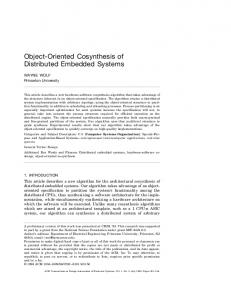
C. Related work Similar to our approach, Eles et al. [9] use a graph-based method to calculate schedules for a hardware architecture consisting of processors, ASICs, and shared buses. Their notion of a Conditional Process Graph is used for analyzing control and data-flow dependencies of tasks that were already assigned to processors. Similar to Pop et al. [10], their focus is on scheduling. In contrast, our method provides inter alia a basis for scheduling but focuses on the deployment of mode tasks extracted from COLA models. The graph structure we are presenting is generated in a fully automated way from our COLA model and fits perfectly into the overall MDD process. Moreover, it provides all necessary information to generate C code and configure the platform. A middleware for distributed real-time systems is used to map inter-task communication. D. Organization In the following section, we motivate the usage of socalled mode automata to express distinct system behaviors. This leads to a distinction between different types of COLA clusters which partition the system model. Section II introduces the notion of a Cluster Dependency Graph. Possible task orderings as well as logical addresses are calculated according to this data structure. A case study outlined in Section IV demonstrates our approach using an adaptive cruise control as example. We conclude with an outlook on possible extensions and current work. Throughout the paper we use parts of the model of the case study to illustrate the presented approach. II. S YSTEM O RGANIZATION U SING O PERATING M ODES During our work, it turned out to be very useful to have a way to formulate distinct system behaviors in terms of different operating modes. This prompted us to include a language construct in the Component Language which is commonly called mode automaton in the literature [1], [8], [11]. Fohler [12] describes issues of handling mode changes in the context of MARS [13]. In the case of COLA, the results present at the output ports of the unit which is realized by a mode automaton, depend on the automaton’s current state and the values at the output ports of the particular unit implementing that state. Figure 1 shows a COLA automaton which illustrates the principle of operating modes by means of a fictitious adaptive cruise control system (ACC) used in modern automobiles. Depending on whether the driver switches the ACC system on or off, the mode is altered. This design enables the developer to decouple the modeling process of the—in this case—two different behaviors. This caters for a reduction of system complexity and results in improved software quality. Moreover, the separation into different operating modes advances the reusability of COLA components and therefor contributes to saving development costs. To seize the given example, one can assume that most of the ACC functionality is not used in the mode net_acc_off, whereas in the mode net_acc_on a lot of sensor processing like velocimetry and distance measurement has to be done.

mode==1



mode acc_disp

s_user s_act

net_acc_on

net_acc_off s_mot

dist mode==1

Figure 1.

Operating modes in a fictional adaptive cruise control system.

A. COLA clusters In a tool-backed model-driven development process, not only the modeling of system behavior is in focus, but for the sake of clearness and maintainability different views onto the system at hand are defined and have to be distinguished. Following the nomenclature of Pretschner et al. [14] we distinguish between the logical architecture and technical architecture. The first one describes the functional system behavior whereas the latter contains target hardware platform information and other non-functional requirements. Operating modes are initially defined in the logical architecture. In order to clarify the transition from the logical to the technical architecture, we introduce the notion of a cluster in the following. In the course of advancing from the logical to the technical architecture, the question arises in which way COLA units have to be mapped onto tasks from the operating system’s point of view. Such a task is called cluster in the technical architecture. Actually the process of clustering a COLA system is done manually. Yet, in a future version, a fully automated workflow is intended for this activity. In the following, we are assuming the availability of such a clustered COLA system. No matter how we got the clustering—manually or fully automated—a valid one has to fulfill the clustering condition: the set of all clusters C has to cover the complete COLA system. More precise, a valid clustering of a system is given if and only if clustered(root) is satisfied. Here, root ∈ UI denotes the unique identifier of the top-most unit and UI is the set of all unique identifiers of a COLA system (see also [1] for more details). We distinguish the following two cases: 1) There exists exactly one cluster cl ∈ CL, where CL denotes the set of all clusters, which refers to the unit instance with unique identifier x. In the following, this relation is denoted by cl ∼ x. Furthermore, no sub-unit instances uniquely identified with x .y are allowed to be clustered separately. C1(x) ⇔

∃1 cl ∈ CL : cl ∼ x ∧ ∀x.y ∈ UI . ∄cl ′ ∈ CL : cl ′ ∼ x.y

2) There exists exactly one cluster cl which refers to a unit instance with unique identifier x implementing an automaton (denoted by is atm(x)). Its sub-unit instances

mode==1

net_acc_on

DEV_ROTATION

DEV_TIME

DEV_ULTRA

DEV_TOUCH

DEV_VIEW

DEV_PRGM

rot_sens

time_sens

ultra_sens

touch_sens

view_sens

prgm_sens



net_acc_off

Rotation

Radar

s_act

dist

UI

mode

s_user

mode==1 ACC

ACC_off

ACC_on

acc_disp

s_mot

DEV_DISPLAY

DEV_MOTOR

off

Figure 2. Port correlation: the signature of automata and that of the unit instances implementing the states is the same.

uniquely identified with x .y are clustered. C2(x)

⇔

∃1 cl ∈ CL : cl ∼ x ∧ is atm(x) ∧ ∀x.y ∈ UI : clustered(x.y)

The first-order predicate clustered(·) is defined as follows: clustered(x)

⇔

C1(x) ∨ C2(x)

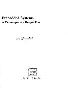
B. Relating mode- and working-clusters As mentioned in the previous section, the entire COLA system model has to be clustered. In this section, we introduce the distinction between different cluster types: mode clusters and working clusters. Mode clusters realize mode automata which are responsible to initiate further control- and data-flow, that is, the next operations to perform. In our terms, these next operations are a set of working or mode clusters. A mode cluster can either be the top-most cluster of a system or can be initiated by another mode cluster. Furthermore, there exists a very important correlation between these two cluster types: input and output ports of an automaton and those of the units realizing the automaton’s different states have the same ports, that is, these units have the same signature and therefor share the same input values. In Figure 2 the dashed lines indicate port correlations, which means that these ports share the same value and actually are identical. III. C LUSTER D EPENDENCY G RAPH Data dependencies which arise due to channels between interconnected units in COLA networks, lead to dependencies in COLA clusters, too. For more complex COLA systems it is administrable to have a clearer understanding of data dependencies which in the sequel will help us to generate schedule plans and C code (see also [15], [16]). Further the contained information serve for the configuration of the used middleware. This middleware will be subject to another paper and will only be roughly discussed where it is necessary for

Figure 3. Section IV.

Cluster dependency graph for the case study introduced in

a better understanding. We’ll give a short introduction into its functionality in Section III-C and IV. Definition 1 (Cluster Dependency Graph): A Cluster Dependency Graph (CDG) is a directed, acyclic graph G = (Vw , Vm , Vb , Ed , Em ) with three types of pairwise disjoint vertices: working cluster vertices Vw , buffer vertices Vb and so-called mode cluster vertices Vm . The set of directed edges is divided into data-flow edges Ed and mode edges Em with Ed ∩ Em = ∅. For the edges it holds: Ed = {(u, v) | u ∈ Vw , v ∈ Vb } ∪ {(u, v) | u ∈ Vb , v ∈ (Vw ∪ Vm )} and Em = {(u, v) | u ∈ Vm , v ∈ (Vw ∪ Vm )}. Solid data-flow edges going out of a working cluster vertex (visualized by a rectangle) and pointing into an octagon (buffer vertex) symbolize that the working cluster vertex writes data into a buffer, whereas an edge pointing from a buffer vertex to an working or mode cluster vertex (symbolized by a diamond) indicate the fact that they read from the buffer. In case of mode cluster vertices, only mode edges (drawn as dashed edges) can start here and the edges can only point to working and mode cluster vertices. This distinction is made in order to emphasize the different exclusive control- and data-flows depending on the current mode. Figure 3 shows an example for a cluster dependency graph of the case study explained in Section IV. A. Data dependencies Data dependencies arise when two or more COLA units are interconnected via channels. Data-flow is then given in the following three cases: 1) Data-flow from an input port of a network to either an input port of a connected sub-unit or to an output port of the network at hand, or 2) between sub-units of a network, that is, from a single output port to at least one input port of another sub-unit, and finally 3) between an output port of a sub-unit and an output port of the surrounding network. These data dependencies between COLA units in the logical architecture are reflected in the technical architecture, that is, dependencies between clusters. These dependencies on the

technical architecture are represented as edges in the CDG. We distinguish between two kinds of edges: solid data-flow and dashed mode edges, as introduced above. Before stating the accurate relation between the logical and technical architecture, let us first introduce necessary notations according to Kugele et al [1]. Let u1 = hn1 , σ1 , c1 , I1 i and u2 = hn2 , σ2 , c2 , I2 i be two units of the COLA system S = hu, U i with u1 , u2 ∈ U , being the set of all units, and u denoting the root unit of the COLA model. σ1 and σ2 are the signatures of both units, that is, the particular vectors of typed input and output ports (accessible using in(σ) and out(σ)). Furthermore, let ch = ha, s, {d1 , d2 , . . . , dk }i be a channel connecting a single source port s with at least one destination port di , with 1 ≤ i ≤ k. Then, two cluster vertices cl 1 (working cluster) and cl 2 (working or mode cluster), are connected by solid edges with a buffer vertex b in between (cl1 → b → cl2 ), if there exist two connected unit instances u1 and u2 (with unique identifiers x1 and x2 ) in the COLA system model, which are associated with these clusters: cl1 ∼ x1 and cl2 ∼ x2 . It holds ∀cl1 ∈ Vw , cl2 ∈ (Vw ∪ Vm ) ∀x1 , x2 ∈ UI : cl1 ∼ x1 ∧ cl2 ∼ x2 =⇒ [∃e1 , e2 ∈ Ed ∃b ∈ Vb : e1 = (cl1 , b) ∧ e2 = (b, cl2 ) ⇔ (∃ch ∈ C ∃x1 , x2 ∈ UI : s ∈ out(σ1 )∧ ∃di ∈ {d1 , . . . , dk } : di ∈ in(σ2 ))] whereas C is the set of all channels in the network containing u1 and u2 . In this scenario, we dictate that u2 is not a subunit of u1 since all sub-units of a network are automatically contained in the same cluster as u1 . But then, for dashed mode edges we have a different characteristics. Let cl 1 be a mode cluster vertex and cl 2 be either a working or a mode cluster vertex. Then, there is a dashed edge connecting these vertices (cl1 99K cl2 ) if u1 is an automaton with a set of states Q, and u2 is the instantiation of one of its states q ∈ Q, denoted by inst(q) = u2 . ∀cl1 ∈ Vm , cl2 ∈ (Vw ∪ Vm ) ∀x1 , x2 ∈ UI : cl1 ∼ x1 ∧ cl2 ∼ x2 =⇒ [∃e ∈ Em : e = (cl1 , cl2 ) ⇔ is atm(x1 ) ∧ ∃q ∈ Q : inst(q) = x2 ] B. Causality and task execution order The cluster dependency graph provides a basis for reasoning about causality and is appropriate to cover the execution order of tasks. In Figure 3 causality is given in the following way: the working clusters Rotation, Radar and UI have to be executed in order to write their results to the suitable buffers s_act, dist, mode, and s_user. In addition, these working clusters are again dependent on the values of their

2

1

6

4

5

9

7

3

8

6

1

5

2

4

3

9

7

8

1

2

7

3

4

8

6

5

9

1

2

3

4

5

6

7

8

9

10

12

11

13

14 15

t

Figure 4.

Examples for feasible task orders.

input buffers which are in turn set by the working clusters DEV_ROTATION, DEV_TIME, and so on. Once the buffers (s_act, dist, mode, and s_user) have been set, the mode cluster ACC can be executed using the data present at its connected buffer vertices. Depending on the active mode, either ACC_off or ACC_on will be executed afterwards and write its results to the respective buffers. Based on this causality, a possible execution order of clusters—tasks in the sense of operating systems—can be derived in a straightforward manner. We have to point out, that there can be a plethora of possible execution orders. The task of our offline-scheduler which is currently under development, is to select the best order with respect to a set of given constraints. In the example given in Figure 3, hundreds of possible execution orders can be found. Some of them are exemplarily presented in Figure 4. For the sake of clarity, cluster names are substituted by their logical addresses given in Figure 5. A very small extract of all possible orderings, the working clusters ACC relies on, is depicted in the gray box. These clusters can be placed in an arbitrary order with respect to the exception that clusters must not be executed before their input buffer(s) are set. Afterwards, the ACC mode cluster is run and finally one of the sequences 10, 12 or 11, 13 is chosen, depending on the result returned by the mode cluster. It is the job of our allocation procedure to assign each task to a specific procesor of a multi-processor platform. In this scenario communication over buses as well as processor capacity utilization with respect to memory and CPU usage has to be taken into account. We will elaborate on our allocation and scheduling procedure in a subsequent paper. Furthermore, regarding multi-core or multi-processor platforms we can state that some of the working cluster tasks can operate in parallel since they are independent from each other, such as DEV_ROTATION, DEV_TIME, DEV_ULTRA, and so forth. Hence, in the example given in Figure 3 there are several independent paths, that is, they do not share a common vertex, from a root vertex to the mode vertex ACC. Paths starting at a working cluster vertex passing different buffer vertices, each of them has to be a child of the starting vertex, and ending again in the same cluster vertex (working or mode) are count as one path. Hence all those sub-paths have a length of exactly two, such as the sub-path starting at UI and ending at ACC. Vertices on independent paths starting at root vertices and ending in ACC (excluded) could be deployed on different processors in order to make use of parallelism where possible

1

2

16

17 7 22

3

4

18

5

19

6

20

8 24

25

14 15

Figure 5.

view_sens

DEV_S_ TOUCH

touch_sens

DEV_S_ PRGM

prgm_sens

mode

net_ui

21

9

23



DEV_S_ VIEW

acc_disp s_user

net_ACC_on_off s_mot

s_act

DEV_S_ ROTATION

rot_sens

DEV_S_ SYSTIME

time_sens

DEV_S_ ULTRA

ultra_sens

DEV_A_ DISPLAY

DEV_A_ MOTOR

net_rotation

10

11

26

27

12

13

Logical addresses for the case study.

and beneficial. C. Logical address generation As mentioned before, the presented approach for a dependency graph is intended for use in a MDD process. Haberl et al. [15] presented an approach to generate code fully automatically, to minimize the possibility of programming faults. In order to use the process for development of distributed systems, it is necessary to allow for communication during runtime. Each channel between two clusters, which is transformed into C code and thus turn into tasks during runtime, indicates the need for a communication link at runtime. As described before, buffers are used for temporary storage of data sent from one cluster to another. These buffers correspond to memory allocated by the middleware used on the execution platform. It is, amongst others, the middleware’s task to enable for transparent and timely communication between the running tasks. The middleware can be managed using a configuration file which contains information about the sizes and addresses of local and remote buffers. The dependency graph provides assistance during construction of this configuration file as well as the correct addressing of middleware API calls while generating the C code for each cluster. Every buffer vertex in the graph is given a logical address, which will be used later on in the development process for middleware configuration and appropriate read and write calls by the connected clusters. Of course, the logical addresses of all buffer vertices have to be different to avoid race conditions. In addition to inter-cluster communication, there is a need for storing the state of each cluster. As the hypothesis of perfect synchrony assumes the periodic invocation of each unit, we use a time-triggered scheduling scheme. Thus each generated task is started over and over again. In order to keep the tasks’ states between invocations, the middleware saves their local variables. This state buffering is realized using a logical address, too. Each cluster vertex in the dependency graph is assigned its private logical address for this purpose. When executed, a task’s first job is to read its state using the assigned address. Accordingly, the last instruction before the task’s termination writes the actualized state back to the middleware. Figure 5 shows a possible addressing for the

dist

net_radar

Figure 6.

The ACC main diagram.

dependency graph introduced in Figure 3. As described, each buffer in this example is assigned an address pointing to an appropriately sized data buffer. The addresses reserved for the tasks’ state storage are enlisted as well. While the stated concept for saving states is true for both kinds of clusters, a mode cluster is given an additional address. As we explained in Section II-B, mode clusters decide on which clusters to be executed next. The information about their decision which state to execute is not depicted using a channel in the functional model, but by means of hierarchy. All working clusters contained in a unit implementing a state, form the active cluster set. But as there is no channel in the functional model, the cluster graph does not contain a buffer for filing this decision. That is the reason why mode clusters are given an additional address. Considering our example graph, this is true for the ACC mode cluster. Figure 5 states both addresses for that cluster. When being executed, the mode cluster stores a numeric value, which points to a mode, at that logical address. As the middleware is the first instance to see the decision about the active mode, it hands the tasks realizing the functionality of that mode over to the operating system’s dispatcher for execution. IV. C ASE S TUDY In the following we will exemplify the usage and the benefits of our dependency graph considering a model for a fictitious adaptive cruise control (ACC). This system is intended to keep an automobile’s velocity at a constant value, while maintaining a defined minimum distance to the car driving ahead. The top-level diagram of the according COLA model is shown in Figure 6. While this is a fictitious model and not derived from any real implementation, it is well suited to demonstrate our concepts in this paper. The COLA unit shown in this diagram is a network containing several sources, sinks (both are indicated by solid rectangles in the upper right corner) and other sub-units. Sources and sinks refer to sensors and actuators of the real system, while the rest of the shown sub-units implements the ACC’s behavior. In the following we will refer to this diagram in order to exemplify some concepts. The dependency graph for the ACC example has already been given in Figure 3. As can be seen in the figure, the



*

Figure 7. C code.

/

_

425

COLA network net_rotation which has been translated into

graph consists of a single mode cluster, namely ACC, 13 working clusters, 12 buffers and their respective connections. First we want to detail on the inter-cluster communication. In comparison to the examples presented by Haberl et al. [15], the code generation has been altered to interface the middleware mentioned before, inserting the logical addresses filed in the dependency graph. This enhancement allows for distributed execution of the ACC example code. An example for the altered code representing the working cluster net_rotation, which is depicted in Figure 7, can be seen in Listing 1. In lines 6, 7, and 10 data are read from or written to the buffers which are connected to the working cluster in Figure 5. This realizes the inter-cluster communication described before. The example also shows, how the task reads its actual state in line 5 and writes back the actualized state in line 11. 1 2 3 4 5 6 7 8 9 10 11 12

void net_rotation200399() { state_rotation200399 unit_state; int rotation_0, time_1, rotation_out_0; mw_restore_task_state(7, &unit_state); mw_read(16, &rotation_0); mw_read(17, &time_1); rotation_out_0 = ((rotation_0 * 425) / (time_1 - unit_state.delay200513)); unit_state.delay200513 = time_1; mw_write(22, &rotation_out_0); mw_save_task_state(7, &unit_state); }

Listing 1.

Code for net_rotation.

The code for the mode cluster looks a bit different. First of all mode clusters are, per definition, made up solely of automata. Unlike automata used in working clusters, those of mode clusters do not call a function realizing the states behavior, but write a numeric value to the designated middleware address. This can be seen in line 31 of Listing 2, which shows the generated code for the ACC mode cluster of Figure 1. The address is assigned during logical address generation, as described in Section III-C. The numeric value written by the mode cluster identifies the active mode. After execution of the mode cluster, the middleware checks the value stored at this address and initiates the execution of the appropriate working clusters. Another difference in comparison to working clusters is the absence of mw_write() statements for the automaton’s out ports. Only the input ports are read for computing the mode to activate, as depicted in lines 6 through 9. 1 2 3 4 5

void net_acc_on_off200244() { state_acc200244 unit_state; int decision, s_act, dist, mode, s_user; mw_restore_task_state(14, &unit_state);

6 7 8 9 10 11 12 13 14 15 16 17 18 19 20 21 22 23 24 25 26 27 28 29 30 31 32 33

mw_read(22, &s_act); mw_read(23, &dist); mw_read(24, &mode); mw_read(25, &s_user); switch(unit_state.atm_state) { case 0: if ((mode == 1)) { unit_state.atm_state = 1; decision = 1; break; } decision = 0; break; case 1: if ((mode == 1)) { unit_state.atm_state = 0; decision = 0; break; } decision = 1; break; } mw_write(15, &decision); mw_save_task_state(14, &unit_state); }

Listing 2.

Code for net_ACC_on_off.

V. C ONCLUSIONS In this paper we introduced the concept of a Cluster Dependency Graph. We showed that this formalism is well suited to capture the dependencies arising from data-flow models using COLA as an example language. We defined clusters as distributable entities which build up the partitioned system model. The definition of clusters together with the dependency graph enables for unattended generation of application code. This results in code including the functionality captured by the model as well as the communication needs imposed by the allocation of clusters onto a distributed system. Therefor, channels included in the data-flow model are mapped to logical addresses. These addresses are then attached to the corresponding vertices of the graph. Later on in the development process this information is used by the code generator when inserting communication calls to, and generating a configuration file for, the middleware. Additionally, the dependency graph forms a basis for automatic construction of feasible system schedules and provides a clue for distribution of tasks to the available system nodes. These extension are subject of current research and will be discussed in future work. R EFERENCES [1] S. Kugele, M. Tautschnig, A. Bauer, C. Schallhart, S. Merenda, W. Haberl, C. K¨uhnel, F. M¨uller, Z. Wang, D. Wild, S. Rittmann, and M. Wechs, “COLA – The component language,” Tech. Rep. TUM-I0714, Institut f¨ur Informatik, Technische Universit¨at M¨unchen, Sept. 2007. [2] The MathWorks Inc., Using Simulink, 2000. [3] A. Bauer, M. Broy, J. Romberg, B. Sch¨atz, P. Braun, U. Freund, N. Mata, R. Sandner, and D. Ziegenbein, “AutoMoDe — Notations, Methods, and Tools for Model-Based Development of Automotive Software,” in Proceedings of the SAE 2005 World Congress, (Detroit, MI), Society of Automotive Engineers, April 2005. [4] P. Caspi, A. Curic, A. Maignan, C. Sofronis, S. Tripakis, and P. Niebert, “From simulink to SCADE/lustre to TTA: a layered approach for distributed embedded applications.,” in LCTES, pp. 153–162, ACM, 2003. [5] G. Booch, J. Rumbaugh, and I. Jacobson, The Unified Modeling Language User Guide. Addison-Wesley, 1998. [6] N. Halbwachs, P. Caspi, P. Raymond, and D. Pilaud, “The synchronous data-flow programming language LUSTRE,” Proceedings of the IEEE, vol. 79, pp. 1305–1320, September 1991.

[7] IEEE Std 830-1998: IEEE Recommended Practice for Software Requirements Specifications. Institute of Electrical and Electronics Engineers, 1998. [8] F. Maraninchi and Y. R´emond, “Mode-automata: a new domain-specific construct for the development of safe critical systems,” Science of Computer Programming, vol. 46, no. 3, pp. 219–254, 2003. [9] P. Eles, K. Kuchcinski, Z. Peng, A. Doboli, and P. Pop, “Scheduling of conditional process graphs for the synthesis of embedded systems,” in DATE ’98: Proceedings of the conference on Design, automation and test in Europe, (Washington, DC, USA), pp. 132–139, IEEE Computer Society, 1998. [10] P. Pop, P. Eles, and Z. Peng, “Schedulability analysis for systems with data and control dependencies,” 2000. [11] F. Maraninchi and Y. Remond, “Mode-automata: About modes and states for reactive systems,” Programming Languages and Systems: 7th European Symposium on . . . , Jan 1998. [12] G. Fohler, “Realizing changes of operational modes with pre runtime scheduled hard real-time systems,” in Proceedings of the Second International Workshop on Responsive Computer Systems, (Saitama, Japan), 1992.

[13] H. Kopetz, A. Damm, C. Koza, M. Mulazzani, W. Schwabl, C. Senft, and R. Zainlinger, “Distributed fault-tolerant real-time systems: The mars approach,” IEEE Micro, vol. 09, no. 1, pp. 25–40, 1989. [14] A. Pretschner, W. Prenninger, S. Wagner, C. K¨uhnel, M. Baumgartner, B. Sostawa, R. Z¨olch, and T. Stauner, “One Evaluation of Model-Based Testing and its Automation,” in Proc. 27th International Conference on Software Engineering (A. Press, ed.), no. ICSE’05, (New York, Manhatten), ACM Press, 2005. [15] W. Haberl, M. Tautschnig, and U. Baumgarten, “Running COLA on Embedded Systems,” in Proceedings of The International MultiConference of Engineers and Computer Scientists 2008, March 2008. [16] I. St¨urmer, D. Weinberg, and M. Conrad, “Overview of existing safeguarding techniques for automatically generated code,” SIGSOFT Softw. Eng. Notes, vol. 30, no. 4, pp. 1–6, 2005.