t
Technical papers
Downloaded 01/12/15 to 143.224.253.234. Redistribution subject to SEG license or copyright; see Terms of Use at http://library.seg.org/
Mapping directional variations in seismic character using gray-level co-occurrence matrix-based attributes Christoph Georg Eichkitz1, Marcellus Gregor Schreilechner1, Paul de Groot2, and Johannes Amtmann1 Abstract Texture attributes describe the spatial arrangement of neighboring amplitudes values within a given analysis window. We chose a statistical texture classification method, the gray-level co-occurrence matrix (GLCM), and its derived attributes, to produce a semiautomated description of the spatial arrangement of seismic facies. The GLCM is a measure of how often different combinations of neighboring pixel values occur. We tested the application of directional GLCM-based attributes for the detection of seismic variability within paleoriver features. Calculation of 3D GLCM-based attributes can be done in 13 space directions. The results of GLCM-based attribute calculation differed depending on the chosen GLCM parameters (number of gray levels, analysis window, and direction of calculation). We specifically focused on how the direction of calculation influenced the computation of attributes, while keeping other parameters constant. We first tested the workflow on a 2D training image and later ran on a real seismic amplitude volume from the Vienna Basin. Based on the GLCM-based attributes, we could map the channel features and extract them as geobodies. Additionally, we generated a new set of directional GLCM-based attributes to detect spatial changes in the seismic facies. By comparing these directional attributes, we could determine areas within the channel features having higher directional variability. Areas with higher tendency to directional variations might be associated with changes in lithology, seismic facies, or with seismic anisotropy.
Introduction Common seismic attributes such as complex trace (Taner et al., 1979), coherence (Bahorich and Farmer, 1995), curvature (Marfurt and Kirlin, 2000), or spectral decomposition attributes (Partyka et al., 1999) use mathematical formulations to capture the geometry or physical properties of the subsurface and can be used to illuminate geologic features of interest. Texture is defined by the spatial configuration of rock units and is more diagnostic of and relevant to deformational fabrics, depositional facies, and reservoir properties than an averaged acoustic property (Gao, 2011). The methodology follows the way a seismic interpreter analyzes seismic amplitudes and waveforms. Among many methods available for texture analysis, we choose a statistical texture classification method known as the gray-level co-occurrence matrix (GLCM) (Haralick et al., 1973) and its derived attributes to produce a semiautomated description of the spatial arrangement of seismic amplitude values. The GLCM was primarily designed for texture classification of 2D images. It is a method widely used in many application domains, such as image classification of satellite imagery (e.g., Frank-
lin et al., 2001; Tsai et al., 2007), sea-ice images (e.g., Soh and Tsatsoulis, 1999; Maillard et al., 2005), magnetic resonance, or computed tomography images (e.g., Kovalev et al., 2001; Zizzari et al., 2011). This methodology has been applied to seismic data for the past 20 years (Vinther et al., 1996; Gao, 1999, 2003, 2007, 2008a, 2008b, 2009, 2011; West et al., 2002; Chopra and Alexeev, 2005, 2006a, 2006b; Yenugu et al., 2010; de Matos et al., 2011; Eichkitz et al., 2013). To calculate GLCMbased attributes on 3D seismic data, it is necessary to adapt the method to work in a 3D space. The number of possible directions increases in comparison with the 2D images. For this research project, we used four horizontal directions (0°, 45°, 90°, and 135°) to determine the directional behavior of seismic amplitude values. The workflow was tested on a data set from the Vienna Basin, Austria; the objective was to illuminate seismic character variability within channel features. Method The GLCM is a measure of how often different combinations of neighboring pixel values occur in an image. For a 2D image, the immediate neighboring pixels can
1 Joanneum Research, Geophysics and Geothermics, Leoben, Austria. E-mail:
[email protected]; marcellus.schreilechner@ joanneum.at;
[email protected]. 2 dGB Earth Sciences, Enschede, Netherlands. E-mail:
[email protected]. Manuscript received by the Editor 14 May 2014; revised manuscript received 30 July 2014; published online 30 December 2014. This paper appears in Interpretation, Vol. 3, No. 1 (February 2015); p. T13–T23, 9 FIGS.
http://dx.doi.org/10.1190/INT-2014-0099.1. © 2014 Society of Exploration Geophysicists and American Association of Petroleum Geologists. All rights reserved.
Interpretation / February 2015 T13
Downloaded 01/12/15 to 143.224.253.234. Redistribution subject to SEG license or copyright; see Terms of Use at http://library.seg.org/
Figure 1. (a) In a 3D case, the number of neighbors for one sample point can be best explained by examining a Rubik’s Cube. (b) The center of the Rubik’s Cube (the red box in panel [b]) has in total 26 neighboring boxes. The boxes are aligned in 13 directions. (c) Analogous to this, a sample point in a seismic volume has 26 neighbors aligned in 13 directions. In the developed workflow, it is possible to calculate GLCM-based attributes along a single direction, a combination of directions (e.g., inline direction, crossline direction, etc.), or all directions at once (after Eichkitz et al., 2013). T14 Interpretation / February 2015
be analyzed in four different directions (0°, 45°, 90°, and 135°). The four directions can also be combined to form an average GLCM. Such computation can eliminate the influences of bed dip and azimuth to a certain degree (Gao, 2007). In 3D data, the number of possible directions increases to thirteen. To illustrate this case, the Rubik’s cube is used (Figure 1a–1c), which is built of 27 smaller cubes. The cube in the center, the turning point in a Rubik’s Cube, is the reference point for which the calculations are performed (Figure 1b). The center point is surrounded by 26 neighboring cubes. If we take the center point and draw lines from it to all neighboring cubes, we get 13 directions (see Figure 1c). As in the 2D case, it is possible to calculate the GLCM in single directions, combine several directions, or calculate an average GLCM. Additionally, our algorithm integrates apparent local structural dip of the data (dip steering, e.g., de Rooij and Tingdahl, 2002). With dip steering, the GLCM input volume is warped along the seismic stratigraphy by following a precalculated 3D dip field. One advantage of dip steering is that the input volume for the GLCM computation does not mix signals from different seismic packages, leading to sharper images that are easier to interpret. For further information on the most common methods to estimate structural dip, we recommend the original works by Barnes (1996), Luo et al. (1996), Marfurt et al. (1998), Bakker (2002), Hoecker and Fehmers (2002), and Tingdahl and de Groot (2003). The first step in GLCM calculation is the transformation of the seismic amplitude volume (usually stored in 32 bit floating point) into a gray-level cube. For seismic data, 16 (4 bit) or 32 (5 bit) gray levels are usually regarded as sufficient. Calculations with a greater number of gray levels do not result in any significant differences in the computed attributes (Chopra and Alexeev, 2006a; Gao, 2007). Calculations with more gray levels result in only minor improvements in resulting images and are costly because of long computation times. Despite these issues, we believe that a higher number of gray levels are important to improve the signal-to-noise ratio (S/N), offering a better delineation of the seismic facies. Enhancement of the S/N can be observed up to approximately 512 (9 bit) gray levels. After that point, only minor changes are observable. We integrate a linked-list approach (Clausi and Jernigan, 1998; Clausi and Zhao, 2002; Clausi and Zhao, 2003) to overcome computational performance issues. A linked list is a sequence of nodes in which each node consists of a data part and a reference to the next node. Using this approach, nonzero matrix entries are skipped and calculation time is no longer a function of the number of gray levels. Only the size of the analysis window affects computation times. From the GLCM, a series of textural attributes can be derived. Haralick et al. (1973) originally introduce 14 attributes. Since then, a few more attributes have been developed and published (e.g., Soh and Tsatsoulis, 1999; Wang et al., 2010). Prior to computing any GLCM-based attributes, the GLCM is transformed by
Downloaded 01/12/15 to 143.224.253.234. Redistribution subject to SEG license or copyright; see Terms of Use at http://library.seg.org/
dividing each entry by the sum of all entries, expressing it as a kind of probability matrix. The GLCM-based attributes can be divided into three general groups. First, the contrast group includes attributes such as contrast, homogeneity, and cluster tendency (Haralick et al., 1973; Wang et al., 2010). The attributes in this group are basically a function of the probability of each matrix entry and the difference between gray levels (i and j). Therefore, these contrast group attributes are related to the distance from the GLCM diagonal. Values close to the diagonal (where i and j are the same) result in lower contrast, whereas the contrast increases as the distance from the diagonal increases. In the sample image (Figure 2), contrast is lower for the 135° direction (Figure 2g) than in the 45° direction (Figure 2f). For the 135° direc-
tion, the matrix entries are aligned around the diagonal where i and j are the same. Second, the orderliness group includes attributes such as energy and entropy (Haralick et al., 1973). Attributes in the orderliness group measure how regularly gray-level values are distributed within a given search window. Unlike the contrast group, attributes in the orderliness group are solely a function of the GLCM probability entries. Third, the statistics group includes attributes such as mean and variance (Haralick et al., 1973). These are the common mean and variance calculated from the GLCM probabilities. We generated a small 2D sample image to demonstrate the GLCM calculation along different directions (Figure 2a). In this example, a northwest–southeast-trending feature was modeled. Gray levels along the main feature
Figure 2. (a) Example for the calculation of GLCM-based attributes using eight gray levels from a synthetic 2D gray-scale image. (b) The gray-scales of the image correspond to discrete values. (c) The number of co-occurrences of pixel pairs for a given search window is counted and a GLCM is generated. In this synthetic case, the analysis window is 7 × 7 and attribute response would be assigned to the center image point. Based on this co-occurrence matrix, several attributes can be calculated. In this example, the GLCM are determined for the (d) 0°, (e) 90°, (f) 45°, and (g) 135° directions and (h) for all directions at once. The first step in calculation is the determination of co-occurrences (figure parts in the middle). Zero entries are marked in gray, and the highest value of each matrix is marked in dark green. It is evident that calculations in single directions lead to sparse matrices. The GLCM is normalized by the sum of the entries to get a kind of probability matrix (figures on the right). Finally, the probabilities are used for the calculation of the GLCM-based attributes. In the column labeled “attribute response,” the results for entropy, contrast, homogeneity, entropy, and cluster tendency are shown.
Interpretation / February 2015 T15
Downloaded 01/12/15 to 143.224.253.234. Redistribution subject to SEG license or copyright; see Terms of Use at http://library.seg.org/
are similar, and the largest variation occurs perpendicular to the main feature. Eight gray levels (3 bit) were used (Figure 2b). The number of gray levels (N g ) defines the rank of the square matrix (Figure 2c). In the example, the GLCM is a square matrix of rank eight. In Figure 2d–2g, the results for GLCM calculations for four directions are shown. Additionally, the results of the combined GLCM calculation in all four possible directions are shown in Figure 2h. Note the high number of zero values inside the matrix, which heavily influences computation times. With the use of a linked-list approach, we can overcome this problem. The calculated GLCM-based attributes energy, homogeneity, and cluster tendency are highest when the calculation is done parallel (135° direction) to the main feature in the tested image. Contrast gives the highest values perpendicular to the main feature. Entropy is smallest in the strike (45°) direction, whereas in other directions, entropy values are higher but similar to each other. From these results, we can see that the attribute response is dependent on the strike of the main feature. The directional behavior of the GLCM-based attributes
Figure 3. The workflow for seismic amplitude variability detection by using GLCMbased attributes is divided into four parts. (a) The first part is the calculation of each GLCM-based attribute in four space directions (in this example, only the four horizontal directions are used). (b) The second step is the determination of minima and maxima values and their direction for each GLCM-based attribute. (c) In step 3, the ratio between maximum and minimum is calculated. The ratio is used to determine a threshold value. (d) The threshold value is applied in step 4 to identify areas with higher directional variability and to visualize only these directions of minima and maxima.
T16 Interpretation / February 2015
can thus be used to estimate variability of the seismic amplitude responses. The input to generate GLCM-based attributes can be seismic amplitude volumes, or any derived seismic attribute volume (coherence, curvature, spectral decomposition). Against this background, we developed a workflow composed of four steps (Figure 3). Currently, the workflow for mapping directional variations operates in 4 directions only, but we intend to extend this to a full analysis of all 13 possible space directions. The first step is the calculation of GLCM-based attributes in four separate space directions (0°, 45°, 90°, and 135°). By integrating dip steering methodology into GLCM calculation, we can increase the S/N. In the second step, we determine for each sample point and each GLCM-based attribute the maximum and minimum values. Additionally, we store the direction in which maximum and minimum values occur for each attribute. Information of maximum and minimum values and their directions are stored in separate cubes. Subsequently, we use this information to identify the direction of high-
Downloaded 01/12/15 to 143.224.253.234. Redistribution subject to SEG license or copyright; see Terms of Use at http://library.seg.org/
est variation in the seismic data. Rarely do we get the same attribute response in all directions, although minimum and maximum values sometimes are very close to each other. In these areas, we would overestimate the directional variability in our seismic data. Therefore, it is necessary to condition the output data to distinguish between areas with high-directional variability and areas with low directional variability. This is done in steps three and four of the workflow. In step 3, we calculate the ratio between maximum and minimum values and set a manually determined threshold value for each attribute. The threshold value is then used in step 4 to set all areas with a ratio below the threshold value to have no directional variability. In areas above the threshold, the minimum and maximum directions are determined. By combining the calculated GLCM-based attributes, we are able to determine areas that tend to have lower directional variability from those areas prone to have more directional variability. Application to a channel system within the Vienna Basin We apply the workflow to a 3D seismic data set from the Vienna Basin (close to the border between Austria and Slovakia). The bin size of the cube is 25 × 25 m (82 × 82 ft). At a depth of approximately 1000 ms, a meandering channel system was interpreted. The channel deposits are most probably of Sarmatian or Pannonian age (Middle to Upper Miocene), and have a width of 130–300 m (426–984 ft) and an average thickness of 70 ms. Strauss et al. (2006) describe similar features in the southern Vienna Basin. The channel system is clearly identified with the help of the coherence attribute (Eichkitz et al., 2012). We interpret the edges of the channel as lineaments on several time slices (Figure 4) and use the interpreted lineaments as guidance for the interpretation of the GLCM-based attribute displays. For comparison, the GLCM-based attributes (energy, homogeneity, contrast, entropy, and homogeneity) were computed in four directions (0°, 45°, 90°, and 135°) with and without dip steering applied to the input seismic amplitude volume. Sixty-four gray levels were used for GLCM-based calculation. In the energy and cluster tendency attributes, the channel system is well imaged (Figure 5) because the surrounding rocks show very low, uniform values and the channel filling has high values in both attributes. In the homogeneity and entropy attributes, the channel system is still visible, but it is more difficult to differentiate the channel from the surrounding strata. The homogeneity attribute is more difficult to interpret because the surrounding areas have many spots with responses similar to that inside the channel system. For the contrast attribute, the interpretation of the channel system is very difficult. No real differentiation between the channel and the surrounding rocks is possible. As noted, all attributes were calculated in four horizontal space directions with and without dip steering. In general, the results using dip steering have a higher
S/N (Figure 6), so we decided to use the results with dip steering for the determination of spatial variation in seismic data. In the energy attribute display, large variations are observed in all four space directions. Visual
Figure 4. In the tested data set, multiple channel features are observed. To visualize these channel features and to interpret the channel edges, coherence time slices were used (Eichkitz et al., 2012). In panel (a) is a time slice of the amplitude and in panel (b) is a time slice of semblance-based coherence. The interpretation of the channel edges is displayed in panel (c). Coherence interpretation is overlain on all GLCM-based attribute plots. Interpretation / February 2015 T17
Downloaded 01/12/15 to 143.224.253.234. Redistribution subject to SEG license or copyright; see Terms of Use at http://library.seg.org/
analysis of these four different images (Figure 7) leads to the conclusion that calculation in the inline direction gives the highest values for this attribute. According to theory and supported by the test image (Figure 2), highenergy values can be interpreted as the direction in which the least variation occurs. The 135° direction (northwest–southwest) generally shows the lowest energy response. This can be interpreted as the direction
in which the highest variation in seismic data response is present. Ratio cubes for each attribute volume were generated in the next step. For each GLCM-based attribute, the maximum value is divided by the minimum value. Based on these ratio cubes, we manually set the threshold values. For energy and entropy, a threshold value of 1.2 is best for illuminating the channel interior. For
Figure 5. GLCM-based attributes calculated along 0° direction (east–west): (a) Energy, (b) contrast, (c) homogeneity, (d) entropy, and (e) cluster tendency. The channel structure can clearly be seen in the energy and cluster tendency attribute. The contrast attribute in this direction reveals little information about the channel structure. In panel (f) , the coherence time slice is shown once more for comparison reasons. T18 Interpretation / February 2015
Downloaded 01/12/15 to 143.224.253.234. Redistribution subject to SEG license or copyright; see Terms of Use at http://library.seg.org/
homogeneity and cluster tendency, a threshold value of 1.1 was used. Using these values, we produce the final images of direction of maximum and minimum GLCM-
based attribute values. Figure 8 shows the direction of maximum values. Within the channel features, the maximum values mostly occur in the 0° and 90° direc-
Figure 6. An important step in seismic attribute calculation is to take the structural dip into account. For this purpose, we determine the structural dip by using a complex trace analysis, a discrete scan, or a gradient structure tensor approach. In this work, the discrete scan was found to produce best results. In panels (a and c), the images represent the calculation without using the structural dip. In panels (a and b), several seismic traces are shown. Clearly, one can see that the vertical positions of peak amplitudes are not aligned in one single horizontal line. By neglecting the structural dip of the data, the center of our analysis window would fall at the dark gray line in panel (a) and our analysis window would be a perfect cube. Calculation of GLCM-based energy in the 0° direction (c) without steering and (d) with steering. In the steered computation, the S/N is higher and certain features can better be imaged (see the gray arrows).
Figure 7. GLCM-based energy attribute calculated in four different space directions. In panel (a), the zero direction (east–west), in (b), the 90° direction (north–south), in (c), the 45° direction (northeast–southwest), and in (d), the 135° direction (northwest–southeast) are shown.
Interpretation / February 2015 T19
Downloaded 01/12/15 to 143.224.253.234. Redistribution subject to SEG license or copyright; see Terms of Use at http://library.seg.org/
Figure 8. Direction of maximum values for four GLCM-based attributes: (a) energy, (b) homogeneity, (c) entropy, and (d) cluster tendency. Additionally, in panel (e), an amplitude time slice is shown. T20 Interpretation / February 2015
Figure 9. Direction of minimum values for four GLCM-based attributes. (a) energy, (b) homogeneity, (c) entropy, and (d) cluster tendency. Additionally, in panel (e), an amplitude time slice is shown.
Downloaded 01/12/15 to 143.224.253.234. Redistribution subject to SEG license or copyright; see Terms of Use at http://library.seg.org/
tions. Only in a few spots, especially in the western area, does the 135° direction (northwest–southeast) dominate. In Figure 9, the directions of minimum values are shown. In the minimum value cubes, the 45° direction (northeast–southwest) dominates over the entire image and the 135° direction is present only in a few parts of the image. The 0° and 90° directions rarely occur in the minor direction cubes. Based on Figures 8 and 9, most spatial variation in seismic character within the channel features can be found in the 45° direction (northeast–southwest). In contrast, we see the lowest spatial variations in the 90° direction. Within the project area, no well log information is available, so it is not possible to directly verify the interpretation. Conclusions The results of GLCM-based attribute calculations may differ depending on the GLCM parameters (the number of gray levels, analysis window, and direction of calculation) chosen. In this study, we fix the number of gray levels at 64, the analysis window for all calculations at 3 × 3 × 11, and only varied the direction of calculation (0°, 45°, 90°, and 135°). By using this approach, we obtain a set of cubes containing direction-dependent values for each attribute. Based on these directional attributes, it is possible to determine directions in which the specific attribute exhibits maximum or minimum values. Maxima and minimums are correlated with directions in which the seismic response shows the highest and lowest variations. The workflow was applied to a data set from the Vienna Basin with the objective of illuminating river/channel features. In this case study, the channel features can clearly be identified with the help of the GLCM-based attributes. By applying directional GLCM calculation, it is possible to map areas with higher and lower tendencies to have directional variability in attribute response. These attribute responses may be correlated with anisotropy in the channel fillings. Acknowledgments We thank OMV Exploration & Production for providing the data set and funding this research project, as well as for giving permission to publish the data. We would like to give special thanks to N. Bird and J. Davies for improving our use of English and organization of the text. Constructive reviews by I. Marroquín, D. Gao, and one anonymous reviewer helped to improve an early version of this paper. References Bahorich, M., and S. Farmer, 1995, 3D seismic discontinuity for faults and stratigraphic features: The coherence cube: The Leading Edge, 14, 1053–1058, doi: 10.1190/1 .1437077. Bakker, P., 2002, Image structure analysis for seismic interpretation: Ph.D. dissertation, Technische Universiteit Delft. Barnes, A. E., 1996, Theory of 2D complex seismic trace analysis: Geophysics, 61, 264–272, doi: 10.1190/1.1443947.
Chopra, S., and V. Alexeev, 2005, Application of texture attribute analysis to 3D seismic data: 75th Annual International Meeting, SEG, Expanded Abstracts, 767–770. Chopra, S., and V. Alexeev, 2006a, Application of texture attribute analysis to 3D seismic data: The Leading Edge, 25, 934–940, doi: 10.1190/1.2335155. Chopra, S., and V. Alexeev, 2006b, Texture attribute application to 3D seismic data: 6th Annual International Conference and Exposition on Petroleum Geophysics, SEG, Expanded Abstracts, 874–879. Clausi, D. A., and M. E. Jernigan, 1998, A fast method to determine co-occurrence texture features: IEEE Transactions on Geoscience and Remote Sensing, 36, 298– 300, doi: 10.1109/36.655338. Clausi, D. A., and Y. Zhao, 2002, Rapid extraction of image texture by co-occurrence using a hybrid data structure: Computers and Geosciences, 28, 763–774, doi: 10.1016/ S0098-3004(01)00108-X. Clausi, D. A., and Y. Zhao, 2003, Grey level co-occurrence integrated algorithm (GLCIA): A superior computational method to rapidly determine co-occurrence probability texture features: Computers and Geosciences, 29, 837–850, doi: 10.1016/S0098-3004(03)00089-X. de Matos, M. C., M. Yenugu, S. M. Angelo, and K. J. Marfurt, 2011, Integrated seismic texture segmentation and cluster analysis applied to channel delineation and chert reservoir characterization: Geophysics, 76, no. 5, P11– P21, doi: 10.1190/geo2010-0150.1. de Rooij, M., and K. Tingdahl, 2002, Meta-attributes — The key to multivolume, multiattribute interpretation: The Leading Edge, 21, 1050–1053, doi: 10.1190/1.1518445. Eichkitz, C. G., J. Amtmann, and M. G. Schreilechner, 2012, Enhanced coherence attribute imaging by structural oriented filtering: First Break, 30, 75–81. Eichkitz, C. G., J. Amtmann, and M. G. Schreilechner, 2013, Calculation of grey level co-occurrence matrix-based seismic attributes in three dimensions: Computers and Geosciences, 60, 176–183, doi: 10.1016/j.cageo .2013.07.006. Franklin, S. E., A. J. Maudie, and M. B. Lavigne, 2001, Using spatial co-occurrence texture to increase forest structure and species composition classification accuracy: Photogrammetric Engineering and Remote Sensing, 67, 849–855. Gao, D., 1999, 3D VCM seismic textures: A new technology to quantify seismic interpretation: 69th Annual International Meeting, SEG, Expanded Abstracts, 1037–1039. Gao, D., 2003, Volume texture extraction for 3D seismic visualization and interpretation: Geophysics, 68, 1294– 1302, doi: 10.1190/1.1598122. Gao, D., 2007, Application of three-dimensional seismic texture analysis with special reference to deep-marine facies discrimination and interpretation: Offshore Angola, West Africa: AAPG Bulletin, 91, 1665–1683, doi: 10.1306/08020706101.
Interpretation / February 2015 T21
Downloaded 01/12/15 to 143.224.253.234. Redistribution subject to SEG license or copyright; see Terms of Use at http://library.seg.org/
Gao, D., 2008a, Adaptive seismic texture model regression for subsurface characterization: Oil & Gas Review, 6, 83–86. Gao, D., 2008b, Application of seismic texture model regression to seismic facies characterization and interpretation: The Leading Edge, 27, 394–397, doi: 10.1190/1.2896632. Gao, D., 2009, 3D seismic volume visualization and interpretation: An integrated workflow with case studies: Geophysics, 74, no. 1, W1–W12, doi: 10.1190/1.3002915. Gao, D., 2011, Latest developments in seismic texture analysis for subsurface structure, facies, and reservoir characterization: A review: Geophysics, 76, no. 2, W1– W13, doi: 10.1190/1.3553479. Haralick, R. M., K. Shanmugam, and I. Dinstein, 1973, Textural features for image classification: IEEE Transactions on Systems, Man, and Cybernetics, 3, 610–621, doi: 10.1109/TSMC.1973.4309314. Hoecker, C., and G. Fehmers, 2002, Fast structural interpretation with structure-oriented filtering: The Leading Edge, 21, 238–243, doi: 10.1190/1.1463775. Kovalev, V. A., F. Kruggel, H.-J. Gertz, and D.Y. von Cramon, 2001, Three-dimensional texture analysis of MRI brain datasets: IEEE Transactions on Medical Imaging, 20, 424–433, doi: 10.1109/42.925295. Luo, Y., W. G. Higgs, and W. S. Kowalik, 1996, Edge detection and stratigraphic analysis using 3D seismic data: 66th Annual International Meeting, SEG, Expanded Abstracts, 324–327. Maillard, P., D. A. Clausi, and H. Deng, 2005, Operational map-guided classification of SAR sea ice imagery: IEEE Transactions on Geoscience and Remote Sensing, 43, 2940–2951, doi: 10.1109/TGRS.2005.857897. Marfurt, K. J., and R. L. Kirlin, 2000, 3D broad band estimates of reflector dip and amplitude: Geophysics, 65, 304–320, doi: 10.1190/1.1444721. Marfurt, K. J., R. L. Kirlin, S. L. Farmer, and M. S. Bahorich, 1998, 3-D seismic attributes using a semblance-based coherency algorithm: Geophysics, 63, 1150–1165, doi: 10.1190/1.1444721. Partyka, G., J. Gridley, and J. Lopez, 1999, Interpretational applications of spectral decomposition in reservoir characterization: The Leading Edge, 18, 353–360, doi: 10.1190/1.1438295. Soh, L.-K., and C. Tsatsoulis, 1999, Texture analysis of SAR sea ice imagery using gray level co-occurrence matrices: IEEE Transactions on Geoscience and Remote Sensing, 37, 780–795, doi: 10.1109/36.752194. Strauss, P., M. Harzhauser, R. Hinsch, and M. Wagreich, 2006, Sequence stratigraphy in a classic pull-apart basin (Neogene, Vienna Basin): A 3D seismic based integrated approach: Geological Carpathica, 57, 185–197. Taner, M. T., F. Koehler, and R. E. Sheriff, 1979, Complex seismic trace analysis: Geophysics, 44, 1041–1063, doi: 10.1190/1.1440994. Tingdahl, K. M., and P. F. M. de Groot, 2003, Post-stack dip- and azimuth processing: Journal of Seismic Exploration, 12, 113–126.
T22 Interpretation / February 2015
Tsai, F., C.-T. Chang, J.-Y. Rau, T.-H. Lin, and G.-R. Liu, 2007, 3D computation of gray level co-occurrence in hyperspectral image cubes, in A. F. Yuille, S.-C. Zhu, D. Cremers, and Y. Wang, eds., Energy minimization methods in computer vision and pattern recognition: Springer, 429–440. Vinther, R., K. Mosegaar, K. Kierkegaard, I. Abatzi, C. Andersen, O. V. Vejbaek, F. If, and P. H. Nielsen, 1996, Seismic texture classification: A computer-aided approach to stratigraphic analysis: 65th Annual International Meeting, SEG, Expanded Abstracts, 153–155. Wang, H., X.-H. Guo, Z.-W. Jia, H.-K. Li, Z.-G. Liang, K.-C. Li, and Q. He, 2010, Multilevel binomial logistic prediction model for malignant pulmonary nodules based on texture features of CT image: European Journal of Radiology, 74, 124–129, doi: 10.1016/j.ejrad.2009.01.024. West, B. P., S. R. May, J. E. Eastwood, and C. Rossen, 2002, Interactive seismic facies classification using textural attributes and neural networks: The Leading Edge, 21, 1042–1049, doi: 10.1190/1.1518444. Yenugu, M., K. J. Marfurt, and S. Matson, 2010, Seismic texture analysis for reservoir prediction and characterization: The Leading Edge, 29, 1116–1121, doi: 10.1190/1 .3485772. Zizzari, A., U. Seiffert, B. Michaelis, G. Gademann, and S. Swiderski, 2001, Detection of tumor in digital images of the brain: in M. H. Hamza, ed., Proceedings of the IASTED International Conference Signal Processing, Pattern Recognition and Applications, IASTED/ACTA Press, 132–137.
Christoph Georg Eichkitz received an M.S. (2005) in applied geophysics from the Montanuniversitaet Leoben, Austria, where his research was focused on modeling of microgravity data. He joined Joanneum Research, Institute of Geophysics and Geothermics, in 2007, where he is responsible for seismic interpretation, attribute calculation, and structural modeling. His main interest is application of seismic attributes for reservoir characterization. He is finishing his Ph.D. study on the application of textural attributes for seismic interpretation at the Montanuniversitaet Leoben.
Marcellus Gregor Schreilechner received an M.S. (1996) and Ph.D. (2007) in applied geosciences from the Montanuniversitaet Leoben, Austria, where he is also a lecturer for applied geophysics. He is the head of the Institute of Geophysics and Geothermics at Joanneum Research, the second largest nonuniversity research organization in Austria. His main interests are the sequence
Downloaded 01/12/15 to 143.224.253.234. Redistribution subject to SEG license or copyright; see Terms of Use at http://library.seg.org/
stratigraphic interpretation of seismic reflection data, interpretation of well log data, and application of seismic attributes for reservoir characterization.
cal topics and coauthored a patent on seismic object detection. Together with F. Aminzadeh, he wrote a book on soft computing techniques in the oil industry.
Paul de Groot is the president of dGB. He received M.S. and Ph.D. degrees in geophysics from Delft University of Technology. He worked for 10 years at Shell, where he served in various technical and management positions. He subsequently worked for four years as a senior research geophysicist for TNO Institute of Applied Geosciences before cofounding dGB in 1995. He has authored many papers covering a wide range of geophysi-
Johannes Amtmann received a B.S. (2007) and an M.S. (2009) in applied geosciences from the Montanuniversitaet Leoben, Austria. For the past seven years, he has been working at Joanneum Research, Institute of Geophysics and Geothermics, where he is responsible for acquisition and interpretation of well log data. His main interests are interpretation of image logs and application of seismic attributes for reservoir characterization.
Interpretation / February 2015 T23