and acts as a resampling filter: all the intersection points between the input .... The entry (i, j) of the 2D pointers data structure XY , for example, points to the list of ...
Marching Intersections: an Efficient Resampling Algorithm for Surface Management C. Rocchini, P. Cignoni, F. Ganovelli, C. Montani, P. Pingi, R. Scopigno Istituto di Scienza e Tecnologie dell’Informazione Consiglio Nazionale delle Ricerche Loc. San Cataldo, Pisa - Italy frocchini j cignoni j ganovelli j montani j pingig@iei:pi:cnr:it r:scopigno
@
cnuce:pi:cnr:it
Abstract
remove small imperfections due to the acquisition process (small holes corresponding to parts of the object unseen by the input device) or high frequency details often due to acquisition noise. In this paper we present a resampling filter which transforms a complex surface presenting small topological imperfections and/or high frequency details into a new, watertight, valid triangulated surface in which approximation error is a user controlled parameter. The filter operates by firstly transforming the input surface into a new simple representation scheme in which only the intersections between the surface and the lines of a user-selected regular grid are represented; then a new, approximated boundary model is reconstructed from these intersections. For a simpler exposition, we refer our method in the paper by using the terms filter and filtering: it has to be underlined that the algorithm is actually based on a surface resampling approach rather than on a classical vertex smoothing [28]. Our method is called Marching Intersections (MI). Marching Intersections actually indicates the original algorithm for the surface reconstruction phase and the name has been clearly borrowed from the well-known Marching Cubes (MC) [18] algorithm for the extraction of isosurfaces from scalar volume datasets. MI and its main characteristics (simplicity and speed of the discretization step, compactness of the representation per intersections, efficiency of the reconstruction and quality of the output surfaces) are presented in detail in Section 2. Besides being a simple and efficient surface resampling filter, MI gives also good results when used in other applications. The method can be used, for example, for the conversion between different geometric representation schemes, for the topological simplification of complex models, for the geometric simplification of huge meshes (i.e. meshes
The paper presents a simple and efficient algorithm for the removal of small topological inconsistencies and high frequency details from surface models. The method, called Marching Intersections (MI), adopts a volumetric approach and acts as a resampling filter: all the intersection points between the input model and the lines of a user selected 3D reference grid are located and then, beginning from these intersections, an output surface is reconstructed. MI, which presents good characteristics in terms of efficiency, compactness, and quality of the output models, can be also used: for the conversion between different representation schemes; to perform logical operations on geometric models; for the topological simplification of surfaces; and for the simplification of huge meshes, i.e. meshes too large to be allocated in main memory during the simplification process. All these aspects are discussed in the paper and timing and graphic results are presented.
1 Introduction Thanks to the great diffusion of devices for the acquisition of the shape of 3D objects and to the constant improvement of the performances (and prices) of graphic cards, the use of 3D digital freeform geometric models is rapidly increasing in many applications, ranging from the reverse engineering to the authoring of 3D virtual worlds. In most cases, the 3D models are represented by the description of their boundary surfaces and these surfaces are very often represented by means of triangles. When the number of triangles is high (as, for example, in the case of automatic acquisition through range scanning) we can have not only rendering problems, but also problems connected to the editing and manipulation of the surfaces in order to 1
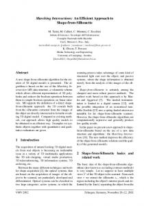
Figure 1. The MI algorithm in a 2D example: (top-left) the curve to be processed and the two data structures collecting the intersections between the input curve and the vertical (top-center) and horizontal (top-right) lines of the user selected grid; (bottom-left) based on the horizontal and vertical intersections, an MC look up table entry code is located for each not empty (virtual) cell; (bottomright) the reconstructed curve. It has to be noted that the vertical intersections inside the small dotted box are collected and then deleted from the algorithm because belonging to the same virtual cell and this leads to the removal of high frequency details.
too large to be loaded in core memory), for the evaluation of logical operations between models (carving, sculpting). We briefly present some of these applications in Section 3 and show some of the results we got. Moreover, a modified version of MI has been used for merging multiple range maps in 3D scanning applications; a detailed description of this method has been presented in [23]. Conclusions are outlined in Section 4. We do not provide an all-inclusive state of the art Section: references to the related works are distributed on the different applications of the method.
lines of the grid are stored in proper data structures (discretization step); from these structures the redundant intersections are then removed (top-middle and top-right images in the Figure) and, finally, the output surface is reconstructed by means of a technique which reminds the MC algorithm and makes use of the MC’s look up table for the triangulation of each active (virtual) cell. The details of the method are given in the following Sections 2.1-2.3.
2.1 Surface Discretization The discretization step consists in detecting all the intersections between the input surface and the reference grid. To simplify the computations, all the geometric coordinates of the input data are immersed in the space of the selected grid; the goal of this scaling transformation is to have all the grid lines lying on integer values; this improves the efficiency of the computations and the management of the intersections between the input meshes and the grid edges. The discretization of the input mesh occurs on a per-face basis. For each input triangle, its axis-aligned bounding box is determined and then three different 2D conversion steps
2 The Marching Intersections Algorithm As briefly summarized in the Introduction, the method presented in this paper is a resampling filter for the removal of small topological anomalies and high frequency details from a surface. A 2D example of the different steps of the algorithm is shown in Figure 1: given the curve to be processed, the user chooses the reference grid which meets her/his approximation requirements (top-left); all the intersections of the input curve with the horizontal and vertical 2
Figure 2. An example of the Removal of two discordant intersections belonging to the same virtual cell.
are performed. For each scan conversion step, we compute the intersections between the triangle and the orthogonal set of grid lines. This process leads to the construction of the 2D dynamic data structures XY , XZ , and ZY containing the intersections between all the input faces and the corresponding grid lines (the top-middle and top-right images in the 2D example of Figure 1).
Figure 3. Reconstruction of a virtual cell and of the corresponding triangular patch performed by the MI method (from left to right, top to bottom), starting from a signed intersection on an edge.
The entry (i; j ) of the 2D pointers data structure XY , for example, points to the list of intersections between the input surface and the grid line parallel to the Z axis and passing through the point [i; j; 0].
2.2 Surface Reconstruction The basic idea of the (MI) reconstruction method is very simple: the reconstruction of a 3D surface is completely defined if all the signed intersections of the surface with the lines of a regular grid are known. The main steps of MI are shown in Figure 3: the reconstruction of the surface parcel contained in a virtual cell of the reference grid. As described in the previous Section, the initial scale transformation performed on the input data allows the nodes of the grid to lie on integer coordinates (i, j , k , . . . ); given a virtual grid cell it is therefore easy to find the intersections lying on its edges. The MC-like classification of the vertices of a virtual cell can be obtained easily from the analysis of the intersections existing on its edges. If an edge contains an intersection, than the classification of its vertices depends on the orientation of the intersection, i.e. the value of the sign field sg (see Figure 3). For each classified (i.e. interior/exterior) cell vertex v , the classification of the adjacent vertex v 0 on an incident edges e is concordant with v if no intersections exist on e, or discordant if a single intersection exists with direction compatible with the class of vertex v . If the intersections configuration along the current cell edges are MC-compatible, then we return the corresponding 8-bit binary code. This code allows to access the standard MC look-up table and to reconstruct the encoded triangular patch. In our algorithm, we use a MC look up table which solves the problem of the ambiguity in the reconstruction of the triangular patch internal to a grid cell [19]. Different traversal strategies have been proposed for visiting the cell grid in surface fitting. The classic MC approach is in general implemented by adopting an iterative
Each intersection is represented in the dynamic data structures by means of the numeric value (ic) of the intersection (for the XY data structure, for example, the field holds the z component of the intersection) and by the sign (sg) of the observation (if we suppose to walk along the grid line onto which the intersection has been located, a ”+” sign means that we are entering the object, a ”-” means we are leaving it). At the end of the scan conversion process, each list is sorted with respect to the intersection value. Sorting ensures fast detection of nearby intersections and fast search for specific intervals. The only geometric operation the intersections undergo is the removal: each pair of consecutive intersections i1 and i2 which lie on the same cell edge (that is, bici1 c = bici2 c) and have discordant signs (sg i1 6= sgi2 ) is removed from the structure it belongs to. As shown in Figure 2, this operation corresponds to a resampling which implies the removal of high frequency details and has the effect to get an arrangement of the intersections data structures in a MC-compliant manner, i.e. in such a way that a MC-like surface reconstruction algorithm could be successfully applied. Even though the intersection data structures do not explicitly represent a 3D grid, it is quite easy to reconstruct the virtual cells of the grid by simply locating the corresponding edges in the XY , XZ , and Y Z data structures. Arranging the data structures in a MC-compliant way means, for example, to ensure the existence of no more than one intersection on each virtual cell edge. 3
slice-based visit of all the cells of the volume. Another solution visits the cells following a propagation approach [15], tracking the surface from an initial seed cell. This solution has advantages (e.g. allows to produce output encoded in triangle strips), but implies the handling of a huge stack for the addresses of the active cells to be visited (with impact on space and time efficiency). Moreover, a propagation approach is more effective if the output surface is ensured to consist of just one component. The algorithm we designed performs an iterative visit of the intersection lists, which presents the efficiency of the propagation methods because only the active cells are analyzed and the simplicity of the slice-based MC visit because a stack to remember the visited cells is not needed. We visit, in sequence, the three data structures XY , XZ , Y Z ; for each structure, we analyze the entries from left to right and from bottom to top. We do not have to maintain trace of the processed cells because we adopt the following visiting strategy:
is intersected by one or more grid lines, then some notcanonical cells configurations can be produced in the reconstruction phase of MI. MI code is designed to detect these not-canonical cells and to manage them appropriately. All the virtual cells which contain intersections and have not been safely reconstructed by MI are considered to cover part of a hole on the object surface; all the edges of the triangles generated in neighbor cells which lie onto faces of the current cell are inserted into an auxiliary edge list which encodes the boundaries of the holes; these edges are then analyzed: starting from a seed edge, the boundary of a hole is reconstructed by simply connecting edges with compatible extremes. The hole is then triangulated by means of a simple 3D extension of a 2D triangulation algorithm [21]. The only hypothesis is that the boundary of the hole is simple and not self-intersecting.
2.4 Evaluation
� XY
Marching Intersections turned out to be efficient both in the discretization step (because the location of the intersections model-grid is computationally cheaper than the computation of the 3D primitive to voxel distances which is typical of the approaches based on distance volumes) and in the reconstruction step (the algorithm moves on the intersections and therefore on the active cells of the virtual grid. The compactness of the method comes from the compactness of the data structures for the representation of the intersections; the total memory occupancy depends on the (user driven) quality and resolution of the output rather than on the size of the input. In the following Sections we will discuss about the theoretical and experimental error MI introduces on the models.
data structure: for each intersection of the XY structure, the four virtual cells sharing the edge the intersection belongs to are analyzed. The cells presenting other XY intersections, besides the one under examination, already considered by the algorithm (i.e. already analyzed in the left-to-right, bottom-to-top visit of the structure) are discarded because the internal triangular patch has already been produced. In our implementation, the analysis of the four cells exploits the coherence of the common cell faces;
� XZ data structure: in an analogous way, for each inter-
section of the XZ structure the four cells sharing the edge the intersection belongs to are analyzed. Here, the cells discarded are those presenting already visited XZ intersections as well as XY intersections;
3 Applying the Marching Intersections Algorithm
� YZ
data structure: for each intersection of the Y Z structure the four corresponding cells are analyzed. We discard the cells presenting already visited Y Z intersections as well as the XY and XZ intersections.
As stated in the Introduction, we basically propose MI as a filter for freeform triangulated surfaces. In this Section we analyze the results obtained in filtering meshes but we also report some possible applications of the method: the evaluation of implicit models, the realization of logical operations between3D objects, the topological simplification of complex models, the geometric simplification of huge meshes.
When the surface fitting process fails on some cells (see next subsection), MI stores the addresses of these cells in an auxiliary structure for further processing.
2.3 Locating and Closing Holes
3.1 Filtering Surfaces and Removing High Frequency Details
Our resampling filter permits to remove small holes from the input surfaces. Small surface holes which are completely contained in the interior of a single grid cell are, by construction, automatically removed from the output mesh. If, conversely, the ideal surface patch which fills the hole
We are not aware of many papers specifically dealing with the problem of filtering surfaces. For a long time, this 4
Table 1. Results obtained running MI on a set of input models. Times are comprehensive of the I/O times. I/O times actually represent most of time spent for processing the St. Matthew (more than 90 millions of faces) dataset. Input Data name St. Matthew
Vase
Bunny
size (# triangles) 90,731,545
2,104,096
69,451
grid (# virtual cells) �10M �1M �100K �10M �1M �100k �500k �100k �10k
time (mm:ss.t) 21:11.0 21:01.0 21:00.0 0:24.3 0:17.5 0:16.2 0:2.4 0:1.9 0:1.7
Michelangelo Project 1 ;
problem has been under-estimated because most of the geometric models originated from CAD systems and these systems generally contain automatic tools for avoiding anomalies. However, Barequet et al. [2] presented a system, called RSVP, for repairing the boundary representation of CAD models. Two types of errors are considered: topological errors (aggregate errors, like zero-volume parts, duplicate or missing parts, etc.) and geometric errors due to numerical inaccuracy errors (like cracks or overlaps of geometry). The output of the system describes clean and consistent twomanifolds (possibly with boundaries) with derived adjacencies. RSVP is powerful but mainly addressed to CAD models. With the large diffusion of devices for the automatic acquisition of the shape of objects, filtering surfaces for removing little inconsistencies or noise is a common need. With reference to the geometric representation schemes based on regular grids, a number of different proposals have been presented, based on the use of octrees or regular grid to encode distance fields (scalar fields that specify the minimum distance to a shape [7, 10]) or simple grids whose data values are obtained by filtering and sampling techniques [14]. However, we do not want to deepen this aspect because we are not proposing a new representation scheme (in this sense, for example, distance fields offer a greater completeness): we propose MI as a simple surface-to-surface filter based on resampling. In this sense our solution does not assure, at least from a theoretic point of view, that all the high frequency details are removed from the input model. Table 1 reports some of the results we obtained testing MIon three sample datasets:
�
MI Output size (# triangles) 435,844 89,670 18,083 523,052 109,912 22,782 48,746 16,187 3,201
� �
Vase: a laser-scanned vase, represented by a fairly big mesh (2,104,096 triangular faces); Figure 7 shows the filtered meshes; Bunny: the Stanford Bunny mesh (35,947 vertices, 69,451 triangular faces), courtesy of the Stanford Computer Graphics Laboratory 2.
Times are comprehensive of the I/O times. We are not interested here in stressing the ability of our method to perform geometric simplification; we want simply underline the high efficiency of the algorithm (the hardware used for the experiments was a 350Mhz Pentium2 with 256MB of main memory), its compactness (no need to explicitly represent grids or cells), and the high quality of the output surface with respect to the adopted grid (all the vertices of the output mesh belong to the input surface). Removing high frequency details introduces an approximation error in the output surfaces. From a theoretical point of view the largest error that can be introduced is equal to the diagonal of the cell of the user selected reference grid. We compared a number of input models with the corresponding output surfaces by means of the METRO tool [5]: the average error introduced is � 1=10:000 of the diagonal of the virtual cell.
3.2 Representation Scheme Boolean Operations
Conversion
and
Due to the simplicity and efficiency of the conversion processes, MI can be used in the conversion of geometric
St. Matthew: a model of Michelangelo’s St. Matthew statue, laser-scanned by Marc Levoy et al., Digital
1 http://graphics.stanford.edu/projects/mich/ 2 http://www-graphics.stanford.edu/
5
inside1 = inside2 = false; last_op = OPRT(inside1,inside2); i1 = list1.begin(); i2 = list2.begin(); while(i1 != list1.end() || i2 != list2.end()) {if(i2 == list2.end() || i1->ic < i2->ic) {last_ic = i1->ic; inside1 = (i1->sg < 0); ++i1; } else {last_ic = i2->ic; inside2 = (i2->sg < 0); ++i2; } op = OPRT(inside1,inside2); if(op != last_op) {list3.push( Insert(last_ic, op?1:-1) ); last_op = op; } }
// // // // // //
initialize the inside/outside status evaluate the binary operator on void i1,i2 are the iterators of the two intersections lists while not end lists... if intersection i1 is lower than i2
// compute new inside/outside status and // go to the next list element
// compute new inside/outside status and // go to the next list element // evaluate the current binary operator // if the inside/outside status changes // we insert a new intercept
Figure 4. The "C" code for the generic logical operation OPRT between the two models list1 and list2. ic and sg represent intercept and sign of the generic intersection.
models between different representation schemes: models represented in a spatial-partitioning or constructive solid geometric, volumetric or mathematical (parametric) schemes, formed by just one connected component or more components, can all be converted into triangulated surfaces by adopting MI. Many papers in the literature faced the problem of the conversion between different representation schemes. Kaufman [16], for example, proposed algorithms to convert surfaces into volumes; Montani and Scopigno [20] dealt with the conversion between octrees and surfaces. With respect to other techniques, MI presents a wider applicability. Likewise to the ray tracing technique [13], MI requires only the definition of a ray intersection function in order to be used on a generic data representation scheme. When the representation scheme is implicit (for example a CSG model) it needs an explicit evaluation step in the conversion process, or when boolean operations between distinct surfaces have to be performed, then MI can be efficiently used. The complex problem of implementing logical operations between surfaces reduces to simple operations on intervals. Figure 4 shows, in ”C” language, the few steps needed for the generic boolean operator OP RT . In order to perform a boolean operation the MI algorithm moves on couples of corresponding lists (list1 and list2 in the example) in the representation structures of the two input models. For each list the intersections are analyzed in geometric order. The resulting intersections (collected in list3) are those causing a change of state (inside/outside the model) on the base of the current position and of the boolean operation performed. Figure 5 shows the results of some logical operations between a sphere and a cube. The operations have been performed in the space of the intersections, after the discretiza-
Figure 5. Three simple logical operations between a Sphere (A) and a Cube (B). A \ B on the left, A [ B in the center, and B A on the right.
tion of the two input parametric models.
3.3 Topological Simplification Most of the papers dealing with object simplification refers to geometrical simplification. Numerous are the algorithms belonging to this class and many are the approaches adopted. In-depth and exhaustive surveys of the algorithms for the reduction of geometric primitives can be found in [11] or [22]. In this section we restrict ourselves to the analysis of the algorithms which allow the modification (and reduction) of mesh topology. The algorithm proposed by Schroeder [25] extends a previous topology preserving solution [27]. The vertices of the input mesh are first classified according to their local topology and geometry, and an error is assigned to them. The vertices are then inserted into a priority queue in which high priority means small error introduced. The decimation is performed by eliminating vertices and the incident triangles. With respect to the geometry simplification algorithm, the re-triangulation is performed by collapsing one edge and this can imply topology modifications (closing of holes or 6
Figure 6. MI in the topological simplification. Upper row: the simple Temple dataset (first image), the MI output (second image) and the resulting model simplified by means of QSlim (third image); the results obtained by running QSlim directly on the Temple dataset (fourth image). Lower row: the simple Cubes dataset (first image), the MI output (second image) and the resulting model simplified by means of QSlim (third image); the results obtained by running QSlim directly on the Cubes dataset (fourth image).
creation of non-manifold parts). The algorithm by El-Sana and Varshney [9] identifies and removes holes, protuberances or cavities by means of �-hulls, a concept very similar to the concept of �shapes [8] in the reconstruction of surfaces from unorganized points. The algorithm is used together with a method (Simplification Envelopes [6]) for the reduction of the geometric primitives. Rossignac and Borrell [24] use a uniform grid to facilitate the clustering of the vertices of the input model. The vertices belonging to a cell of the grid are combined and replaced with a new vertex. The topology of the affected triangles is updated and this implies the elimination of triangles or the updating of their connectivity lists. As a general statement we can observe that previous methods are efficient but can return not-valid surfaces and can present a limited control over the topological reduction. Andujar et al. [1] propose a method based on the space decomposition approach. The data structure used is a version of the well-known octree and the reconstruction of the surface is performed by a MC like algorithm. The MC does not need to compute intersections by means of linear interpolations because the discretization step leads to a binary model. Filters are finally used to smooth the returned surfaces and a classic algorithm for geometrical simplification
is applied. The algorithm proposed by He et al. [14] uses a voxel model for the discretization of the input model and then applies a MC like algorithm to reconstruct the surface. The authors use an adaptive MC in order to get a reduction of the returned geometric primitives. The value assigned to each voxel node is the signed distance between the node and the input surface. Fitting a surface means to extract the isosurface at threshold zero. The methods based on a space decomposition approach generally present a low efficiency, due to the representation conversion, but ensure a good control over the topology reduction rate and the geometric validity of the returned surfaces. The space decomposition methods do not work in an incremental way and this implies that the applications requiring many levels of detail (LOD), for example interactive rendering or transmission, cannot obtain LODs as partial results of a single simplification process. Apart from the special cases in which a coarser LOD is obtained by grouping together eight adjacent voxels, each LOD requires a new discretization and surface fitting process. MI shows some similarities with the algorithm proposed by He et al. [14]. However, MI makes use of resampling rather than filtering; it does not assign signed distance values to the nodes of the grid and the nodes themselves are 7
not explicitly represented. The points computed in the discretization step belong to the input model and they are the only vertices of the output surfaces. These characteristics make our algorithm very attractive and more efficient, more accurate and more thrifty in the use of memory than the existing space decomposition methods. MI’s efficiency and speed justifies its iterative use with different grid sizes when multiple LODs are required. However, it has to be noted that MI shares with other methods based on space decomposition some characteristic disadvantages: topological features reduction depends on the size and the placement of the grid in the 3D space with respect to the input mesh; long and thin objects (a knife blade, for example) could be undesirably removed. Two simple examples of the use of MI in the topological simplification are shown in Figure 6: the two models (Temple and Cubes, both formed by 16 parallelepipeds/cubes, 192 triangles) have been first simplified by using MI (second image of each row) and then geometrically simplified by means of a public domain geometric simplifier (QSlim [12], third image of each row). The direct use of a topology not-preserving simplifier on the input dataset could produce topological errors; see, for example, the results obtained by QSlim when it is applied to the original datasets (rightmost images in Figure 6).
The hierarchical structure proposed in [4] is a very general OOC data representation structure and it easily supports high quality simplification; the drawback is represented by the higher execution times and the complex implementation (at least, if compared to the straightforward implementation of clustering). On the other hand, the accuracy of the mesh produced by a clustering approach is very low if compared with the accuracy of methods based on edge collapse. Running times of clustering solutions are obviously impressive, but the quality of the results produced is directly dependent on the regular sub-sampling operated on the mesh (to reach a drastic simplification of a 3D scanned mesh the cluster cell size is generally set much larger than the mean face size). Moreover, clustering produces meshes with a high number of complex (i.e. non 2-manifold) vertices, and this can be a problem in many applications. When a time-efficient removal of high frequency details or small features on a huge mesh is requested, then a possible alternative to the use of standard simplification tools (in case, OOC-oriented) could be to adopt the MI algorithm. Analogously to the clustering approach, MI is an on-line solution (each face is considered only once), has an empirical complexity linear to the mesh size and the cardinality of the output can be easily controlled by an appropriate sizing of the reference grid. Moreover, the removal operations over nearby intersections can be directly performed during the discretization process. Conversely, an important difference with respect to clustering method is that MI produces topologically clean, 2-manifold meshes. Improved results, in term of simplified mesh accuracy, can be obtained by using the MI algorithm in pipeline with one of the existing in-core high-quality simplification algorithms. MI can reduce the complexity of a huge mesh down to the largest size tractable by an in-core simplifier (e.g. a few million faces), and then the in-core simplifier can reduce further the mesh under a more sophisticated control of geometric accuracy. Fig. 7 shows three different decimation levels of the Vase model obtained by adopting three different sizes of the grid reference cell.
3.4 Simplifying Huge Meshes Very large triangle meshes, i.e. meshes composed by millions of faces, are becoming common in many applications. Obviously, these complex meshes introduce severe overhead in transmission, rendering, processing and archival. Mesh simplification and LOD management have become a mature technology that in most cases can efficiently reduce the above overhead. Unfortunately, most of the more recent and efficient geometric simplification tools as, for example, QSlim [12], VTK [26], and Jade [3], require the whole mesh to be loaded in main memory (and use also auxiliary data structures). The RAM size often represents the real bottleneck of the whole process. Only a few algorithms have been recently proposed which solve this problem by means of an Out-Of-Core (OOC) approach to geometric simplification. Among them, Lindstrom [17] proposed an OOC simplification approach, based on vertex clustering, which is efficient in time and space. Cignoni et al. [4] represent the input meshes by means of a hierarchical octree-like data structure which allows to maintain the data on external memory and to load dynamically into main memory only selected sections while preserving data consistency during local updates. They adopt a classical edge-collapse approach, which becomes slightly slower in their OOC implementation if compared to standard RAM-based implementations.
4 Concluding Remarks A new method, called Marching Intersections, for the removal of small topological anomalies and high frequency details from 3D surfaces has been presented. MI can be efficiently used in the conversion between different geometric schemes for the representation of 3D models and for the execution of boolean operations between models, for the topological (as well as geometric) simplification of complex models, and for the geometric simplification of huge meshes (i.e. meshes too large to be allocated in main memory). 8
Figure 7. Three decimated levels of the Vase model (originally, 2,104,096 triangles): 523,052, 109,912, and 22,782 triangles for the left, center, and right image, respectively.
References
In our opinion, the most relevant aspects of the MI method can be summarized as follows:
�
�
�
[1] C. Andujar, D. Ayala, and P. Brunet. Validity preserving simplification of very complex polyhedral models. In Michael Gervaut, Dieter Schmalstieg, and Axel Hildebrand, editors, Proceedings of 5TH Eurographics Workshop on Virtual Environments, pages 1–10. SpringerVerlag Wien, 1999.
efficiency: MI locates the intersections between the input model and the lines of the user selected grid, rather than the distances of the input surfaces from the nodes of the grid; in the surface reconstruction step, the algorithm moves on the intersections and therefore only the active cells are visited, without the need to store the addresses of the already visited cells;
[2] G. Barequet, C.A. Duncan, and S. Kumar. RSVP: A geometric toolkit for controlled repair of solid models. IEEE Transactions on Visualization and Computer Graphics, 4(2):162–177, April 1998.
compactness: though the method adopts a volumetric approach, the discretized volume is not explicitly represented; each intersection simply requires a floating point intercept value (ic) and a bit for the sign (sg ); the memory required is proportional to the number of output vertices (the topology of the output faces is implicit) and it does not depend on the complexity and size of the input model.
[3] A. Ciampalini, P. Cignoni, C. Montani, and R. Scopigno. Jade v.2: a Multiresolution Decimation Tool. Visual Computing Group, CNR-CNUCE, Pisa (ITALY), URL http://vcg.iei.pi.cnr.it/enhadecimation.html, 1997. [4] P. Cignoni, C. Montani, C. Rocchini, and R. Scopigno. External memory management and simplification of huge meshes. Technical Report B4-02-03, I.E.I. – C.N.R., Pisa, Italy, Nov 2000.
quality: all the vertices of the output model belong to the input surface; though the maximum theoretical error introduced by the method is equal to the diagonal of the cell of the user-selected reference grid, our tests demonstrated that the practical error is � 1=10:000 of the cell diagonal.
[5] P. Cignoni, C. Rocchini, and R. Scopigno. Metro: measuring error on simplified surfaces. Computer Graphics Forum, 17(2):167–174, June 1998.
Acknowledgements
[6] J. Cohen, A. Varshney, D. Manocha, G. Turk, H. Weber, P. Agarwal, F. Brooks, and W. Wright. Simplification envelopes. In Computer Graphics Proc., Annual Conf. Series (Siggraph ’96), ACM Press, pages 119– 128, Aug. 6-8 1996.
We acknowledge the financial support of the Progetto Finalizzato Beni Culturali of the Italian National Research Council (CNR). 9
[7] B. Curless and M. Levoy. A volumetric method for building complex models from range images. In Comp. Graph. Proc., Annual Conf. Series (Siggraph ’96), pages 303–312. ACM Press, 1996.
[19] C. Montani, R. Scateni, and R. Scopigno. A modified look-up table for implicit disambiguation of Marching Cubes. The Visual Computer, 10(6):353–355, 1994. [20] C. Montani and R. Scopigno. Quadtree/octree to boundary conversion. In J. Arvo, editor, Graphics Gems II, pages 202–218. Academic Press, 1991.
[8] Herbert Edelsbrunner and Ernst P. M¨ucke. ThreeDimensional alpha shapes. ACM Transactions on Graphics, 13(1):43–72, January 1994. ISSN 07300301.
[21] A. Narkhede and D. Manocha. Fast polygon triangulation based on seidel’s algorithm. In A. W. Paeth, editor, Graphics Gems V, pages 394–397. Academic Press, 1995.
[9] Jihad El-Sana and Amitabh Varshney. Topology simplification for polygonal virtual environments. IEEE Transactions on Visualization and Computer Graphics, 4(2):133–144, April 1998.
[22] E. Puppo and R. Scopigno. Simplification, LOD, and Multiresolution - Principles and Applications. In EUROGRAPHICS’97 Tutorial Notes (ISSN 1017-4656). Eurographics Association, Aire-la-Ville (CH), 1997 (PS97 TN4).
[10] S. F. Frisken, R. N. Perry, A. P. Rockwood, and T. R. Jones. Adaptively Sampled Distance Fields: A general representation of shape for computer graphics. In Computer Graphics Proc., Annual Conf. Series (Siggraph ’00), pages 249–254. ACM Press, 2000.
[23] C. Rocchini, P. Cignoni, C. Montani, and R. Scopigno. The Marching Intersections algorithm for merging range images. Technical Report B4-61-00, I.E.I. C.N.R., Pisa, Italy, June 2000.
[11] M. Garland. Multiresolution modeling: Survey & future opportunities. In EUROGRAPHICS’99, State of the Art Report (STAR). Eurographics Association, Aire-la-Ville (CH), 1999.
[24] J. Rossignac and P. Borrel. Multi-resolution 3D approximation for rendering complex scenes. In B. Falcidieno and T.L. Kunii, editors, Geometric Modeling in Computer Graphics, pages 455–465. Springer Verlag, 1993.
[12] M. Garland and P.S. Heckbert. QSlim v.2 Simplification Software. School of Computer Sciences, Carnegie Mellon University, URL: http://www.cs.cmu.edu/˜garland/quadrics/qslim.html, 1999.
[25] W. J. Schroeder. A topology modifying progressive decimation algorithm. In Roni Yagel and Hans Hagen, ´ pages 205–212. IEEE, editors, IEEE Visualization 97, November 1997.
[13] A.S. Glassner. An Introduction to Ray Tracing. Academic Press, 1989.
[26] W.J. Schroeder, K. Martin, and W. Lorensen. The Visualization Toolkit: an Object Oriented approach to 3D graphics. Prentice Hall, URL http://www.kitware.com/vtk.html, 1995.
[14] T. He, L. Hong, A. Varshney, and S. Wang. Controlled topology simplification. IEEE Trans. on Visualization & Computer Graphics, 2(2):171–183, 1996. [15] C.T. Howie and E.H. Blake. The mesh propagation algorithm for isosurface construction. Computer Graphics Forum (Proc. of Eurographics ’94), 13(3):65–74, 1994.
[27] W.J. Schroeder, J.A. Zarge, and W.E. Lorensen. Decimation of triangle meshes. In Edwin E. Catmull, editor, ACM Computer Graphics (SIGGRAPH ’92 Proceedings), volume 26, pages 65–70, July 1992.
[16] A. Kaufman. Efficient algorithms of 3d scanconversion algorithms of polygons. Computers and Graphics, 12:213–219, 1988.
[28] J. Vollmer, R. Mencl, and H. M¨uller. Improved Laplacian smoothing of noisy surface meshes. Computer Graphics Forum, 18(3):131–138, 1999.
[17] P. Lindstrom. Out-of-core simplification of large polygonal models. In Comp. Graph. Proc., Annual Conf. Series (Siggraph 2000), ACM Press, pages 259– 262. Addison Wesley, July 22-28 2000. [18] W. E. Lorensen and H. E. Cline. Marching cubes: A high resolution 3D surface construction algorithm. In ACM Computer Graphics (SIGGRAPH ’87 Proceedings), volume 21, pages 163–170, 1987. 10