J M ( â ) was one of the most eminent figures in Polish mathematics and together with StanisÅaw Zaremba, Leon Licht-.
Wiad. Mat. 48 (2) 2012, 157–171 © 2012 Polskie Towarzystwo Matematyczne
Lech Maligranda (Luleå)
Marcinkiewicz Interpolation eorem and Marcinkiewicz Spaces
J
M (–) was one of the most eminent figures in Polish mathematics and together with Stanisław Zaremba, Leon Lichtenstein, Juliusz Schauder and Antoni Zygmund, the most prominent in analysis. Zygmund considered him as his best pupil, although he had many students in Poland and the USA. We must also remember that it is because of the Master, who was Zygmund, Marcinkiewicz also became a known mathematician. Marcinkiewicz wrote scientific papers in six years (–) and his name in mathematics is connected with the Marcinkiewicz interpolation theorem, Marcinkiewicz spaces, the Marcinkiewicz integral and Marcinkiewicz function, the Marcinkiewicz multiplier theorem, the Jessen–Marcinkiewicz–Zygmund strong differentiation theorem, Marcinkiewicz–Zygmund vector-valued inequalities, Marcinkiewicz– Zygmund inequalities in probability, the Marcinkiewicz–Zygmund strong law of large numbers, Marcinkiewicz–Zygmund inequalities for trigonometric functions and polynomials, the Grünwald–Marcinkiewicz interpolation theorem, the Marcinkiewicz–Salem conjecture, the Marcinkiewicz theorem on the characteristic function, the Marcinkiewicz test for pointwise convergence of Fourier series, the Marcinkiewicz theorem on the Haar system, the Marcinkiewicz theorem on universal primitive functions and the Marcinkiewicz theorem on the Perron integral. I will present the first two parts from these achievements and the description of other parts can be found in my recent paper [31]. Finally, in the third part, the life, scientific career, work and tragic end of Józef Marcinkiewicz is presented.
L. Maligranda
1. e Marcinkiewicz interpolation theorem (1939) e Riesz–orin convexity theorem (, ) and the Kolmogorov result () showing that the conjugate-function operator is of weak type (1, 1) and of strong type (p, p) for 1 < p < ∞ were known for Marcinkiewicz. He tried to prove a theorem containing both these theorems. One of the simple cases of the Marcinkiewicz interpolation theorem is the following result. eorem. If a linear or sublinear mapping T is of weak type (1, 1) and strong type (∞, ∞), that is, satisfies the estimates ∫ λm({x ∈ I : |T f (x)| > λ}) ≤ A | f (x)| dx for any λ > 0, (1) I
ess sup |T f (x)| ≤ B ess sup | f (x)|, x∈I
(2)
x∈I
then T is of strong type (p, p) for 1 < p ≤ ∞, i.e., we have estimate ∫ ∫ 2 1/p p | f (x)|p dx, CA,B ≤ |T f (x)| dx ≤ CA,B A1/p B1−1/p. (3) (p − 1)1/p I
I
e importance of the Marcinkiewicz interpolation theorem is also connected with the so-called weak-Lp spaces. e Lebesgue spaces Lp on the measure space (Ω, Σ, µ) were investigated already in the thirties by F. Riesz for Ω = [a, b] and Ω = Rn . To prove boundedness of several operators it was needed, in the target, to have larger spaces than Lp . Marcinkiewicz observed that the so-called weak-Lp spaces denoted by Lp,∞ (1 ≤ p < ∞) are good candidates and now these spaces are also called Marcinkiewicz spaces. ey are given by one of two quasi-norms: ∥ f ∥p,∞ = sup t1/p f ∗ (t) = sup λµ({x ∈ Ω : | f (x)| > λ})1/p. t>0
λ>0
Note that these spaces are really larger than Lp , since ∫ ∫ | f (x)|p dµ ≥ | f (x)|p dµ ≥ λp µ({x ∈ Ω : | f (x)| > λ}) {x∈Ω:| f (x)|>λ}
Ω
for any λ > 0, that is, ∥ f ∥p,∞ = sup λµ({x ∈ Ω : | f (x)| > λ})
1/p
λ>0
e
weak-L∞
space is here by definition the
≤
(∫
| f (x)|p dµ
Ω
L∞
space.
)1/p = ∥ f ∥p .
Marcinkiewicz interpolation theorem and Marcinkiewicz spaces
Marcinkiewicz published in a two-pages paper [33] and formulated three theorems without proofs. Moreover, he sent a leer, including the proof of the main theorem for p0 = q0 = 1 and p1 = q1 = 2, to Zygmund who aer the war reconstructed all the proofs and published them in (see [48]). is is the reason why Marcinkiewicz interpolation theorem is sometimes called Marcinkiewicz–Zygmund interpolation theorem. Note that in Zygmund presented all the proofs at his Chicago seminar informing that he was only developing Marcinkiewicz’s ideas (cf. [36], p. ). A proof was also given by the PhD students of Zygmund: Mischa Cotlar for p0 = q0 and p1 = q1 (PhD , published in in [12]) and William J. Riordan for 1 ≤ pi ≤ qi ≤ ∞, i = 0, 1, (PhD , unpublished). Marcinkiewicz was probably the first who used the word “interpolation of operators”. Riesz and orin spoke on “convexity theorems” (cf. Peetre [36], p. and Horwath [20], p. ). eorem 1.1 (Marcinkiewicz , Zygmund ). Let 1 ≤ p0 , p1 , q0 , q1 ≤ ∞ and for 0 < θ < 1 define p, q by the equalities 1 1−θ θ = + , p p0 p1
1 1−θ θ = + . q q0 q1
(4)
If p0 ≤ q0 and p1 ≤ q1 (lower triangle) with q0 , q1 , then from boundedness of any linear or sublinear operator T : Lp0 → Lq0 ,∞ and T : Lp1 → Lq1 ,∞ – i.e., T is of weak type (p0 , q0 ) and of weak type (p1 , q1 ) – follows boundedness of T : Lp → Lq (that is, T is of strong type (p, q)) and θ ∥T∥Lp →Lq ≤ C∥T∥1−θ Lp0 →Lq0 ,∞ ∥T∥Lp1 →Lq1 ,∞ ,
(5)
where C = C(θ, p0 , p1 , q0 , q1 ) → ∞ as θ → 0+ or θ → 1− . e Marcinkiewicz interpolation theorem was proved even for pointwise quasi-additive operators, that is, there exists a constant γ ≥ 1 such that for any measurable functions f, g we have the following inequality µ-almost everywhere on Ω: ( ) T( f + g)(x) ≤ γ |T f (x)| + |Tg(x)| .
e Marcinkiewicz interpolation theorem is true if p ≤ q and q0 , q1 , that is, if one point can be in the upper triangle but the point S must appear in the lower triangle. Proof of this theorem was given by: Calderón (), Lions– Peetre (), O’Neil (), Hunt () and Krée (). Berenstein–Cotlar– Kerzman–Krée () proved that if for the segment W0 W1 Marcinkiewicz
L. Maligranda
interpolation theorem is true, then it also holds for another segment obtained from the rotation of W0 W1 around the point S (except horizontal and vertical segments). 1 q
1 W0
0
.
W1
S 1
1 2
1 p
1. Marcinkiewicz interpolation theorem is true in lower triangle: W0 = ( p10 , q10 ), W1 = ( p11 , q11 ), S = ( 1p , 1q ) and q0 , q1 (except horizontal segments)
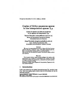
e Marcinkiewicz interpolation theorem is not true in the upper triangle, that is, if p0 > q0 and p1 > q1 . A counter-example is due to Hunt (). He also observed that eorem 1.1 is true in the extended range 0 < p0 , p1 , q0 , q1 ≤ ∞ provided p ≤ q and q0 , q1 (cf. Hunt [21], p. ). 1 q
1 W0 S
0
. W1 1 2
1
1 p
2. Marcinkiewicz interpolation theorem (diagonal case): W0 = ( p10 , p10 ), W1 = ( p11 , p11 ), S = ( 1p , 1p ).
Particular cases of eorem 1.1 have the following form (cf. [19], p. ). eorem (Marcinkiewicz interpolation theorem – diagonal case). If 1 ≤ p0 < p1 ≤ ∞ and T is an arbitrary linear or sublinear operator of weak type (p0 , p0 ) and of weak type (p1 , p1 ), that is, T : Lp0 → Lp0 ,∞ and T : Lp1 → Lp1 ,∞ is
Marcinkiewicz interpolation theorem and Marcinkiewicz spaces
bounded, then it is of strong type (p, p), i.e, T : Lp → Lp is bounded for any θ p0 < p < p1 . Moreover, if 1p = 1−θ p0 + p1 for some 0 < θ < 1, then ∥T∥Lp →Lp ≤ 2
(
p p )1/p 1−θ + ∥T∥Lp0 →Lp0 ,∞ ∥T∥θLp1 →Lp1 ,∞ . p − p0 p1 − p
(6)
eorem (Lile Marcinkiewicz interpolation theorem). If 1 < p ≤ ∞ and T is an arbitrary linear or sublinear operator of weak type (1, 1) and strong type (∞, ∞), that is, T : L1 → L1,∞ and T : L∞ → L∞ is bounded, then it is of strong type (p, p), i.e., T : Lp → Lp is bounded and ( p )1/p 1/p 1−1/p ∥T∥Lp →Lp ≤ 2 ∥T∥L1 →L1,∞ ∥T∥L∞ →L∞ . (7) p−1 In connection to the Marcinkiewicz interpolation theorem we formulate several remarks: 1. Marcinkiewicz’s proof is based on an idea of decomposition of a function which generates later on the concept of the K-functional playing a central role in modern interpolation theory. 2. It is not true, as some authors write, that Marcinkiewicz obtained in his short paper the result related only to the diagonal case. Marcinkiewicz had the theorem in the general case and equations (4) were wrien by q−q q p p−p formulas p0 < p < p1 and q1 −q0 = p00 q11 · p1 −p0 . Moreover, Marcinkiewicz’s second theorem was formulated even for Orlicz spaces in the thesis (in this case it was indeed the diagonal case): if a linear or sublinear operator is bounded T : Lp0 → Lp0 ,∞ and T : Lp1 → Lp1 ,∞, and a function φ : [0, ∞) → [0, ∞) is continuous, (increasing, ) ∫ u vanishing at zero (and satisfy) ing three conditions φ(2u) = O φ(u) , 1 t−p0 −1 φ(t) dt = O u−p0 φ(u) ( ) ∫∞ and u tp1 −1 φ(t) dt = O u−p1 φ(u) as u → ∞, then for f such that ∫1 ∫1 φ(| f |) ∈ L1 [0, 1] we obtain 0 φ(|T f (x)|) dx ≤ C 0 φ(| f (x)|) dx + C, where C is independent of f (see Zygmund [48, m 2] and [49, XII. m 4.22]). 3. E. Stein and G. Weiss () generalized the Marcinkiewicz interpolation theorem replacing the spaces Lpi in the domain of an operator by the smaller Lorentz spaces Lpi ,1 , i = 0, 1 (in fact, they have in the assumption of the Marcinkiewicz theorem only estimates for characteristic functions of measurable sets). Hence, if pi ≤ qi , pi , ∞, i = 0, 1 and q0 , q1 , then the boundedness of T : Lp0 ,1 → Lq0 ,∞ and T : Lp1 ,1 → Lq1 ,∞ implies the boundedness T : Lp → Lq .
L. Maligranda
4. Using reiteration theorems for the real method of interpolation we are geing a generalized Marcinkiewicz interpolation theorem: Suppose 1 ≤ p0 , p1 < ∞, 1 ≤ q0 , q1 ≤ ∞ with q0 , q1 . If a quasi-linear operator T : Lp0 ,1 → Lq0 ,∞ and T : Lp1 ,1 → Lq1 ,∞ is bounded, then T : Lp,r → Lq,r is bounded for any 1 ≤ r ≤ ∞. In particular, T : Lp → Lq,p is bounded. Note that if we have, as in Marcinkiewicz interpolation theorem, p0 ≤ q0 and p1 ≤ q1 , then Lq,p ,→ Lq . 5. A very important progression to a generalization of the Marcinkiewicz interpolation theorem was done by Calderón (), who found the maximal operator in the sense that if an operator T : Lp0 ,1 → Lq0 ,∞ and T : Lp1 ,1 → Lq1 ,∞ is bounded, then (T f )∗ (t) ≤ CSσ ( f ∗ )(t) for all t > 0, where Sσ is the maximal Calderón operator: Sσ f (t) =
∫∞ 0
{
} s1/p0 s1/p1 ds f (s) min 1/q , 1/q t 0 t 1 s ∫tm
= t−1/q0
s1/p0 −1 f (s) ds + t−1/q1
∫∞
s1/p1 −1 f (s) ds,
tm
0
with m = (1/q0 − 1/q1 )/(1/p0 − 1/p1 ). To get Marcinkiewicz interpolation theorem it is enough to investigate boundedness of the last two operators of Hardy type. 6. e Marcinkiewicz interpolation theorem was proved for symmetric spaces by Boyd ( ⇒, ⇔): if 1 ≤ p0 < p1 < ∞, E is a symmetric space with the Fatou property of the norm on either I = (0, 1) or I = (0, ∞) and every linear operator T : Lp0 ,1 → Lp0 ,∞ and T : Lp1 ,1 → Lp1 ,∞ is bounded, then it yields that T : E → E is bounded if and only if 1/p1 < αE ≤ βE < 1/p0 , where the numbers αE , βE are the so-called Boyd indices of the space E defined by ln ∥σa ∥E→E , ln a a→0+
αE = lim
ln ∥σa ∥E→E a→∞ ln a
βE = lim
and σa f (x) = f (x/a)χI (x/a). Krein–Petunin–Semenov () proved that Boyd’s theorem is true for arbitrary symmetric spaces (even without the Fatou property of the norm). In particular, E is an interpolation space between Lp0 and Lp1 . If p1 = ∞, a one-sided estimate for a symmetric space E, βE < 1/p0 , 1 ≤ p0 < ∞, implies that E is an interpolation space between Lp0 and L∞ (see [28, eorem 4.6], where it is proved even for
Marcinkiewicz interpolation theorem and Marcinkiewicz spaces
Lipschitz operators). Moreover, Astashkin and Maligranda [1] proved the following one-sided Boyd theorem: if a symmetric space E has either the Fatou property or it is separable and αE > 1/p1 , 1 < p1 < ∞, then E is an interpolation space between L1 and Lp1 . 7. e Marcinkiewicz interpolation theorem is not true for bilinear operators without additional assumptions.∫ In fact, Strichartz () proved the ∞ following: the operator S( f, g)(x) = 0 f (xt)g(t)dt is bounded S : L1 × L∞ → L1,∞ and S : L2 × L2 → L2,∞ , but it is not bounded S : Lp × ′ Lp → Lp , and Maligranda () proved that the operator T( f, g)(x) = ∫ 1∫ 1 f (s)g(t) min( st1 , 1x ) dsdt is bounded T : L1 × L1 → L1,∞ and T : L2 × 0 0 2 L → L2,∞ , but it is not bounded T : Lp × Lp → Lp for 1 < p ≤ 2. J. L. Lions and J. Peetre () proved that for the real method of interpolation we have the following interpolation theorem for bilinear operators: if a bilinear operator T : Lp0 ×Lq0 → Lr0 ,∞ and T : Lp1 ×Lq1 → Lr1 ,∞ is bounded, then T : Lp × Lq → Lr is bounded, if besides the natural interpolation equality ( ) ( ) ( ) 1 1 1 1 1 1 1 1 1 , , = (1 − θ) , , + θ , , p q r p0 q0 r0 p1 q1 r1 we have also 1/r ≤ 1/p + 1/q − 1. More theorems of this type can be found in papers by Sharpley (), Zafran (), Janson () and Grafakos– Kalton (). 8. e Marcinkiewicz interpolation theorem for spaces of sequences (and some of its analogues) was given by Sargent in . 9. In Y. Sagher introduced the notion of a Marcinkiewicz quasi-cone. If (A0 , A1 ) is a pair of quasi-normed spaces, then a subset Q of A0 + A1 is called a quasi-cone if Q + Q ⊂ Q. Q is a cone if we also have λQ ⊂ Q for all λ > 0. A quasi-cone Q is called Marcinkiewicz quasi-cone in (A0 , A1 ) if (A0 ∩ Q, A1 ∩ Q)θ,p = (A0 , A1 )θ,p ∩ Q
for all 0 < θ < 1, 0 < p ≤ ∞,
where (·, ·)θ,p means the real K-method of interpolation of Lions–Peetre. For : xk ↓ 0} is a Marcinkiewicz quasi-cone in (lp , l∞ ). example, Q = {(xk )∞ k=1 10. In Dmitriev and Krein [13] extended Marcinkiewicz interpolation theorem to operators mapping a couple of Banach spaces (A0 , A1 ) into a couple of Marcinkiewicz spaces (M∗φ0 , M∗φ1 ). e Marcinkiewicz interpolation theorem is cited in several classical books on analysis, harmonic analysis and interpolation theory as, for example, in books mentioned in chronological order in [31].
L. Maligranda
2. Marcinkiewicz spaces Marcinkiewicz investigated three types of spaces: two symmetric spaces and one space of another type, which will be considered in the next part. All are called now Marcinkiewicz spaces. 2.1. Marcinkiewicz function and sequence spaces (). Earlier we informed about the weak-Lp space Lp,∞ (1 ≤ p < ∞) or Marcinkiewicz space given by one of the quasi-norms: ∥ f ∥p,∞ = sup t1/p f ∗ (t) = sup λµ({x ∈ Ω : | f (x)| > λ})1/p, t>0
λ>0
f∗
where denotes the decreasing rearrangement of | f |. e above type of space can be easily generalized. Let I = (0, 1) or I = (0, ∞) and let φ : I ∪ {0} → [0, ∞) be an arbitrary concave function on I such that φ(0) = 0 (it is also possible to take as φ only a quasi-concave function, that is, a function for which the inequality φ(s) ≤ max(1, s/t) φ(t) is true for all s, t ∈ I). e Marcinkiewicz function space M∗φ on I consists of classes of measurable functions given by the quasi-norm ∥ f ∥∗φ = sup φ(t) f ∗ (t) < ∞. t∈I
Another (smaller) Marcinkiewicz function space Mφ on I is generated by the norm ∫t ∗∗ ∗∗ 1 ∥ f ∥φ = sup φ(t) f (t), where f (t) = t f ∗ (s) ds. t∈I
0
In the case where φ(t) = t1/p , 1 < p < ∞ we have M∗φ = Mφ = Lp,∞, but for φ(t) = t we get M∗φ = L1,∞ (weak-L1 space is a quasi-Banach space but not a Banach space, since the triangle inequality holds only with constant 2) and Mφ = L1 . Of course, Mφ ⊂ M∗φ and ∥ f ∥∗φ ≤ ∥ f ∥φ for f ∈ Mφ . e Marcinkiewicz function space Mφ on I is a symmetric Banach space and for an arbitrary symmetric space X on I with the fundamental function φ(t) := ∥χ(0,t) ∥X , Mφ is the largest symmetric space containing X with the same fundamental function, i.e, ∥χ(0,t) ∥X = ∥χ(0,t) ∥Mφ = φ(t) for any t ∈ I. is follows from ∫t t ∥ f ∗ χ(0,t) ∥X for f ∈ X. the fact that 0 f ∗ (s) ds ≤ φ(t) Let us recall that a symmetric space X on I is an ideal Banach space on I (the assumption | f (t)| ≤ |g(t)| almost everywhere on I, g ∈ X and f is
Marcinkiewicz interpolation theorem and Marcinkiewicz spaces
measurable on I implies that f ∈ X and ∥ f ∥X ≤ ∥g∥X ) with the additional property that two arbitrary equimeasurable functions f and g, i.e. satisfying m({x ∈ I : | f (x)| > λ}) = m({x ∈ I : |g(x)| > λ}) for any λ > 0, with f ∈ X and g measurable on I implies that g ∈ X and ∥ f ∥X = ∥g∥X . In particular, ∥ f ∥X = ∥ f ∗ ∥X . Note that when we investigate the Marcinkiewicz spaces Lp,∞ or operators with values in this space, then the so-called Kolmogorov–Cotlar equivalence is important (cf. [17, pp. 485–486]): if 0 < q < p < ∞ and f ∈ Lp,∞, then (∫ )1/q ∥ f ∥p,∞ ≈ sup µ(A)1/p−1/q | f (x)|q dµ . (8) A⊂I 0