69
Marginalizing in Undirected Graph and Hypergraph Models
Enrique F. Castillo
Juan Ferrandiz
Dept. of Applied Mathematics and Computational Sciences. University of Cantabria 39005 Santander, Spain e-mail: castie@ccaix3. unican.es
Department of Statistics and Operations Research, University of Valencia, Dr. Moliner 50, E-46100, SPAIN e-mail:
[email protected]
Abstract
Given an undirected graph g or hypergraph 'H model for a given set of variables V , we introduce two marginalization operators for obtaining the undirected graph YA or hy pergraph 'HA associated with a given subset A c V such that the marginal distribution of A factorizes according to YA or 'HA, respec tively. Finally, we illustrate the method by its application to some practical examples. With them we show that hypergraph models allow defining a finer factorization or performing a more precise conditional independence anal ysis than undirected graph models. 1
INTRODUCTION
In many practical situations the structural relation ship among a set of variables V { V1, . . . , Vn} can be represented as an undirected graph g (V, E) , where E is the set of edges of g. If two variables are indepen dent, the corresponding nodes should not be connected by a path. =
=
Similarly, if the independence between variables X and is indirect and mediated by a third variable Z (that is, if X and Y are conditionally independent given Z), we display Z as a node that intersects the path between X and Y, i. e. , Z is a cutset separating X and Y. This correspondence between conditional in dependence and cutset separation in undirected graphs forms the basis of the theory of Markov fields (Isham [5], Lauritzen [6], Wermuth and Lauritzen [10]) , and has been given axiomatic characterizations (Pearl and Paz [11] ) . Y
However, in many practical cases we can be interested not in the whole set of variables V but in a subset A of them. In this case the initial graph model is not the most appropriate to work with and we are interested in the graph model induced by the initial graph in A. The independence graph of marginal probability distri butions for a subset of the considered variables was un-
Pilar Sanmartin
Department of Mathematics, Jaume I University Castellon, SPAIN e-mail:
[email protected]. es
dertaken in Frydenberg (1990), after Asmussen (1983). There, he stated the collapsibility condition for the corresponding subgraph to be the independence graph of the marginal probability distribution. Unfortunately, not all probabilistic models can be rep resented by undirected perfect maps. Pearl and Paz [11] characterize the dependency models represented by undirected perfect maps. The theorem refers not only to probabilistic but to general dependency mod els. Since the resulting independence graph reveals this lack of sensitivity to detect all independence properties and lack identification of missing n-th (n > 2) order in teractions when second order interactions are present, as an alternative, we use hypergraph models (see Rose [12], Tarjan and Yannakakis [13] , Mellouli [9] , Studeny [16] and Shafer and Shenoy [15] for related problems) . In this paper, based on the factorization properties, we give an algorithm for obtaining the marginal indepen dence graph under general conditions. To illustrate these concepts, we use some examples in which this lack of sensitivity and the characteristic contribution of hypergraph models become apparent. In Section 2 we introduce the main concepts to be used in the rest of the paper with a distinction between those required for the case of graphs and those for hy pergraphs. In particular, we introduce the hypergraph models based on Gibbs distributions. In Section 3 we introduce a marginalization operator for the case of undirected graphs that allows obtaining such a graph in the sense of the marginal model to satisfy the cor responding factorization properties. We also give an algorithm to implement this operator. In Section 4 we follow exactly the same process for the case of hyper graphs. In both sections we illustrate the methods by means of practical examples. Finally, we make some comparisons, and in Section 6 we give some conclu sions and recommendations. 2
BACKGROUND
We divide this section in two parts. The first is devoted to undirected graphs, and the second to Gibbs distri-
70
Castillo, Fernindiz, and Sanmartin
butions and hypergraphs. We assume that the range of every variable is a real set containing the zero. 2.1
UNDIRECTED GRAPHS
The main theorem to be given in Section 3 requires several concepts of undirected graphs which are given below. We illustrate them with some examples. Definition 1 (Path).
Given a graph g a path of length n between nodes Vr and V8 is a sequence of nodes Vo, ..., Vn such that (Vi, Vi+ I); i 0, . . . , n - 1 are edges ofQ and Vo Vr and Vn Vs. =
=
and it contains the only four complete sets of three elements. The remaining complete sets contain one or two elements. Clique: The sets {V1, V3, V4, V5}, {V4, V2}, {V4, V6}, {V7, Vg}, {V7, Vw} , {Vs, Vw} are the cliques ofQ. Boundary Set: The boundary of the set {V1, V3, V4, %} is the set {V2, V6}· The connectivity compo
Connectivity components: nents of the graph g are Tl
{Vl, V2, v3, v4, v5, V6} and T2
=
=
{V7, Vs, Vg , Vw}.
=
Definition 2 (Connected Nodes). Given a graph Q (V, E), two nodes Vr, V8 E V are said to be con nected if there is a path from Vr to Vs. They are said to be directly connected iff the path is of length 1. =
Definition 3 (Complete Set).
Given a graph g
=
(V, E), a set A s:;;: V is said to be complete if all nodes
in A are mutually and directly connected by edges in E. Definition 4 (Clique).
A maximal complete set of
Figure
nodes is called a clique. Definition 5 (Boundary).
Given a graph g
=
(V, E) and a subset A c V the boundary bd(A) of A is the set of nodes Vr tf. A such that they are directly
connected to an element of A, i. e. ,
1:
Undirected graph.
Definition 7 (Completed Edge Set).
Given a graph g (V, E) and a subset A c V, the completed edge sets E * (A) of A is the set of all possible edges between nodes in A. =
Definition 8 (Subgraph). Definition 6 (Connectivity Components).
Given a graph g (V, E) its set of nodes V can be partitioned in maximal subsets of nodes which are mu tually connected (see Lauritzen {1996}, page 6}. These sets are called connectivity components of g. =
Example 1
Consider the set of variables V (V, E) shown in Figure 1, where
{V1, V2, ... , V10} and the graph Q
=
=
Definition 9 (Factorization Property).
A prob ability distribution P on V, is said to factorize ac cording to an undirected graph g (UDC), if for all complete set, C , of vertices there exist non-negative functions '1/Jc such that p(v)
=
Some illustrative examples of the above definitions are: Path: The sequence of nodes {V1, V4, V5, V3} is a path of length 3 between vl and v3, as it is the sequence {V1, V3}, which has length 1. Connected nodes: The nodes V8 and Vg are connected nodes because there is a path {Vs, Vw, V7, Vg} joining VB and Vg. Directly connected nodes: Nodes V7 and Vw are di rectly connected nodes because the path {V7, V1o} join ing them has length l. Complete Sets: The only complete set of four elements in g is {V1, V3, V4, V5} (all pairs of nodes are directly connected). Obviously, all its subsets are also complete
=
graph 9A (A, EIA) , that is, the graph defined over A and containing the edges of E connecting nodes in A.
{(V1, V3), (V1, V4), (V1, V5), (V2, V4), (%, V4), (V3, V5), (V5, V4), (V6, V4), (V7, Vg), (V7, Vw), (Vs, Vw)}.
E
Given a graph g
(V, E) and a subset A C V , the subgraph gA is the
=
IJ
CcV complete
'1/Jc(c)
The above factorization can be done using only cliques. However, this leads to a coarser factorization. Example 2
Consider again the graph in Example
1.
Completed edge set: The completed edge set of the set {V7, Vs, Vg} is {(V7, Vs), (V7, Vg), (Vs, Vg)}. Subgraph:
The subgraph associated with the set
{V2, V4, V5, V6} is {{V2, V4, V5, V6} , {(V2, V4), (V4, V5), (V4, V6)}.
Factorization: A possible factorization of p(v) is p(v)
'1/J(vl, v3, V4, v5)'lj;(v2, V4)'1jJ(v4, v6)'1jJ(v7, vg) 'lj;(v7, vw)'l/J(vs, vlo).
71
Marginalizing in Undirected Graph and Hypergraph Models
2.2
Example 3
Consider the set of variables V {V1,V2,V3, V4,Vs,V6} and the graph 9 (V, E ) , where
GIBBS DISTRIBUTIONS AND HYPERGRAPHS
=
As it is well known undirected graphs do not lead to the finest possible factorization in probabilistic mod els. This justifies the use of the Gibbs and hypergraph models to be given below. Definition 10 (Gibbs Model).
Given a graph 9 (V,E), the set of random variables V is said to follow a Gibbs model according to the graph 9 if its associated probability density function (pdf) can be written in the form
p(v)
=
(
exp -
) / K,
L Uc(c)
CEC
-
=
(1)
=
K
{(1/1, V2),(V1,V3),(V 2,V3),(V4,Vs),(Vs,V6)}
Gibbs Model:
p(v)
ex
II
=
CEC
K
rr
CEC
where the factors in {7/Jc(c)IC E C} are positive. The above interpretation of the joint density in terms of the interaction functions is not unique. However, we are interested in the simplest possible representa tion, which is given by the normalized potential. In it an interaction function Uc(c) appears iff it cannot be written in terms of a sum of functions with less arguments.
A poten tial U such that Uc(c) 0 whenever some component of c is null is called a normalized potential.
Definition 11 (Normalized Potential). =
It can be shown that this potential is unique ( see Win kler (1995) ) . In addition, any given potential U0 can be normalized in the sense of leading to the same joint distribution for V , by means of ( -1)lC\Blujj(b, OD\B) Uc(c) (3) =
L
Definition 12 (Potential Restricted to a Set).
Given a potential U on the set V and a subset A the potential UIA restricted to A is the set UIA {Uc I Uc E U and C c A}. =
c
V
exp(-B12(1+vl)v2 - B13v1v3 -e23V2V3 - e45V4V5 - Bs6VsV6)'
(4)
{6112(1 +vl)V2,813V1V3,823V2V3,845V4V5,856V5V6}· where eij are constants. Normalized Potential:
potential U becomes:
The corresponding normalized
{812V2,812V1V2,813V1V3,823V2V3,845V4V5,856V5V6}· (5) Given the set A {V1,V3, Vs}, the potential restricted to A is:
Potential Restricted to a Set:
UIA
=
=
{B13v1v3}.
Given a set V, an hypergraph is a subset of parts of V.
Definition 13 (Hypergraph).
Definition 14 (Hypergraph asso ciated with a family of potentials. Hypergraph Models).
Given a parametric family of potentials, the hypergraph associated with its normalized potential ue is defined as the class of all sets of V with non-null interaction function ug for at least one element in the family, i. e.: 1{
=
{C c;;; vI ug :j. 0 for some B}.
(6)
The corresponding model is called an interaction junc tions hypergraph or simply hypergraph model. Note that hypergraph models are more capable to dis tinguish models than undirected graph models. For example, the last models cannot distinguish between the hypergraph model with potential (5) and the hy pergraph model with potential
U1
{ 812V2,812V1V2,813V1V3,8123V1V2V3,823V2V3, e45V4Vs,Bs6VsV6}· (7)
Every hypergraph H on V induces in V the graph 9(1-i) (V,E), where =
E
This last equation makes evident that the normalized potential produces a finer factorization (2) of the pdf, because for every non-null interaction function Uc(c) of the normalized potential there is at least one non null interaction function Ujj (d) involving a bigger set of variables.
Let us assume the following density:
with associated potential U0:
{Uc(c)IC E C} in {1} is called a potential.
Note that Expression (1) shows a characteristic factor ization property of the corresponding Gibbs model. In fact the density in ( 1) factorizes as 1 1 exp (-Uc(c)) p(v) 7/Jc(c), (2) =
=
=
where K is a normalizing constant and C is the class of all complete sets of V with respect to 9. The func tions Uc are called interaction functions and some of them can be null. {In order to avoid trivial undeter minations we will assume hereafter u(/J ( ) 0). The set U
E
=
{(Vn Vs) I {Vr, Vs} c;;; A E 7-i}.
The graph 9(1-i) associated with the hypergraph of a family of potentials verifies the factorization property with every probability distribution induced by these potentials. Definition 15 (Hypergraph Partial Ordering).
Given two hypergraphs 1i 1 and 1{2 on V, we say that 1i1 precedes H2 iff every element of 1i1 is contained in an element oj1i2, that is, 1i1 ::5 1i2 q.I::/H1 E H1 3H2 E 1i2 with H1 c;;;
H2
72
Castillo, Ferrandiz, and Sanmartin
Comparing again the potentials in (5) and (7), we can say that the hypergraph associated with (5) precedes the hypergraph associated with (7) , but not conversely.
sets C, we get:
Now we can state the property of normalized poten tials producing finer factorizations in the more pre cise terms of partial ordering of the associated hyper graphs. The hypergraph associated with the normal ized potential precedes the hypergraph associated with any other potential leading to the same probability dis tribution.
c
Let H be the hypergraph and A C V . The boundary hyper graph HA of V \ A is the hypergraph of all subsets of A which are the boundary of some connectivity com ponent of 9v\A in 9(1-l).
Definition 16 (Boundary Hypergraph).
Example 4
The hypergraph associated with the potential U is
{ {V2}, {VI, V2}, {VI, %}, {V2, V3}, {V4, Vs }, {Vs, V6}} .
Graph associated with a hypergrapll.·
ciated with hypergraph H is
j II 1/Jc(c) II 1/Jc(c)dz C