Markov Chain Monte Carlo Computation of Confidence Intervals for ...

Pacific Symposium on Biocomputing 6:203-214 (2001)

MARKOV CHAIN MONTE CARLO COMPUTATION OF CONFIDENCE INTERVALS FOR SUBSTITUTION-RATE VARIATION IN PROTEINS ANDREY RZHETSKY1,2 AND PAVEL MOROZOV1 IColumbia Genome Center, and 2Department of Medical Informatics, Columbia University, 1050 St. Nicholas Avenue, Unit 109, New York, NY 10032, USA {ar345, [email protected]} We suggest a method implemented in a computer program, immodestly dubbed TSUNAMI, that allows us to compare two homologous protein subfamilies with respect to the distribution of substitution rates along sequences. This study furthers our earlier work on a wavelet model of rate variation (1). The current approach allows sensitive detection of subtle discordances in the selection patterns between two protein subfamilies. In addition to performing fast computation of the maximum posterior probability estimates of the relative substitution rates, the method can select the most appropriate number of wavelet parameters for a particular dataset. TSUNAMI is based on a Markov chain Monte Carlo technique, and appears to be more applicable to larger datasets than is the full likelihood-based approach.

1. Introduction Amino-acid sites in real protein sequences differ in their degree of reluctance to accept an amino-acid substitution; furthermore, a particular site’s degree of conservation is usually correlated with its functional importance. Therefore, analysis of relative rates of amino-acid substitution along a protein sequence is essential to our understanding of the evolution of protein function and to our ability to reconstruct phylogenetic trees. Numerous mathematical models have been suggested to describe substitution rate variation (e.g., Durbin and colleagues (2) and the currently popular gamma-model (3, 4)). In a recent paper (1), we presented two alternative models — a wavelet and a Fourier model — that have the attractive property of flexibility in the number of parameters required to describe the rate variation across sites in a particular dataset. Here, we suggest a few enhancements that speed up computation under these models. We also demonstrate how to implement a Bayesian model-selection approach with regard to the wavelet model. We use Markov chain Monte Carlo (MCMC) simulation to compute the posterior distributions of parameter estimates, the posterior-probability confidence intervals for substitution rates, and the maximum posterior density estimates of the parameter values. We speed-up the MCMC computation by fitting the estimates of posterior density to a three-parameter gamma distribution for each rate parameter separately. We implement an MCMC model-selection procedure and apply it to analysis of real sequence data.

Pacific Symposium on Biocomputing 6:203-214 (2001)

2. Trees, likelihood, and pseudolikelihood Before we specify the proposed modifications, we outline the conserved core of the accepted mathematical model of protein evolution. Each set of truly homologous present-day sequences is a product of whole-gene duplications of a whole ancestral gene and local amino-acid substitutions, deletions, and insertions. For many reasons, deletion and insertion events are often excluded from the inference of a phylogeny for a set of homologous proteins, and the statistical modeling and data analyses both concentrate on only substitution events. In practice, the result is that the sites of a multiple alignment that contain at least one deletion character are excluded from analysis, so that the remaining differences among sequences can be explained completely by amino-acid substitution alone. Researchers usually assume that amino acid substitution at each site of a protein sequence follows a Poisson process, whereas the rate of this process varies from site to site. For mathematical description, it is convenient to work with the relative substitution rates for sites, rather than with the absolute rate. The relative rates are simpler because the absolute expected number of amino substitutions per given protein site varies from one branch of the tree to another, whereas the relative substitution rate at each site can be conveniently assumed constant for all branches of the tree. The relative substitution rates for a dataset are usually defined such that the average relative substitution rate over all sites of each dataset is equal to 1. Then, the expected number of substitutions per a unit time at each individual site of the dataset is equal to the product of the relative rate for this site and to the average number of substitutions per site per unit time over all sites. In a typical model, the substitution process is assumed to be homogeneous over time; that is, the intensity matrix, Q, is postulated to be the same for all branches of the true evolutionary tree. Traditionally, the branch lengths of a tree are measured in terms of the number of amino-acid substitutions per site. As long as Q remains constant, the expected lengths of edges are allowed to deviate from the molecular-clock behavior (when all expected root-to-tip distances are equal). The matrix of probabilities of substituting any amino acid for another amino acid over a time interval t at the ith site of protein alignment is computed as a matrix exponential of the product Q t ri, where ri is the relative substitution rate at the ith site. Since Q and t appear in the likelihood equation as an inseparable product, it is convenient to scale Q such that the mean number of substitution per a unit of time is equal to 1 (e.g., see ref. 4). We compute the full likelihood of a tree as a conditional probability of the data given the model and a set of parameter values. In the case of just two sequences, 1 and 2, we compute the likelihood for the xth site as

Lx =

∑ π i P ( i → s1 ( x ), t1 rx )P ( i → s2 ( x ), t2 rx ) i

In this equation, π i is the expected frequency of ith amino acid in the common ancestor of sequences 1 and 2, respectively; s1(x) and s2(x) are the integers (with

Pacific Symposium on Biocomputing 6:203-214 (2001)

value between 1 and 20) corresponding to amino acids at the xth site of sequences 1 and 2, respectively, and notation i → j indicates substitution of amino acid with label i with amino acid with label j. P ( i → s1 ( x ), t 1 r x ) is the probability of observing the ancestral amino acid i substituted with amino acid s1 after time t; and rx is the relative substitution rate at the xth site. Under a time-reversible model equation for likelihood over all sites simplifies to L = P ( s 1 ( x ) → s 2 ( x ), ( t 1 + t2 )r x ) . When we consider more than two sequence simultaneously, the equation for the likelihood function follows the tree topology. We must compute and multiply the probabilities of transitions along each branch of the tree, and then sum such products over all possible values of the unknown amino acids that belong to unobservable ancestral sequences in the interior nodes of the tree. There is a simple and elegant mapping from a ‘parentheses’ encoding of a tree to the matrix equation for Lx. For example, for a hypothetical tree with just four pending vertices - 1, 2, 3, and 4, (6) (5 ) (1) (2) (3 ) (4 ) ( ( ( 1, 2 ), 3 ), 4 ) - we obtain L x = π x × ( Px × ( P x × ( p S ( x ) • p S ( x ) ) • p S ( x ) ) • p S ( x ) ) , 1 2 3 4 where px is a row vector of expected frequencies of amino acids at the root of the tree, (i ) P x = exp ( Qr x t i ) is 20-by-20 matrix of transition probabilities corresponding to the (i) ith branch of the tree, p j is the jth column of this matrix, A × B indicates a regular matrix product, and A • B indicates an elementwise product of two matrices of equal dimensionality, A • B = ( a ij × b ij ) . In complex expressions, operators of elementwise multiplication have a precedence higher than that of operators of the regular matrix multiplication. Clearly, the parentheses pattern is the same in both expressions, commas in tree expression are mapped to pairwise multiplication operators, numerals that represent pending vertices are mapped into corresponding column vectors, and empty spaces between parentheses are mapped to operators of multiplication followed by a full transition probability matrix corresponding to an interior branch. (Matrix notation for likelihood computation comes in handy in MatLab programming, since MatLab computes matrix expressions much faster than it does equivalent scalar expressions.) For a more advanced description of maximum-likelihood analyses in phylogenetics and of the substitution models, please refer to other sources (e.g., ref. 2, pp.192-232: refs. 5, 6). 3. Wavelets and the wavelet model A wavelet decomposition of a discrete function is a mathematical procedure that is used frequently in signal processing and statistical modeling. In addition to their abstract beauty, wavelets have the attractive property of allowing us to compress data by identifying and setting to zero most of the wavelet coefficients that make only small contributions to the signal (7). We briefly introduce wavelets for readers new to this subject. Wavevelets are local discrete functions. They are “local” in that each function has a well-defined domain, and outside of each wavelet, there is a contiguous subset of sites that have zero values. We chose for this study the simplest Haar wavelet, which has value of +1 at the

Pacific Symposium on Biocomputing 6:203-214 (2001)

first half and a value of -1 in the second half of its domain. A wavelet domain length is always a power of 2 (2, 4,..., full sequence) - which is why we had to extend the actual protein sequences in this analysis to the nearest power of 2 by adding dummy unvaried sites. Denoting by the l the sequence length, a complete set of wavelets in our analysis contains l/2 wavelets with domain length 2, which cover the sequences without overlapping way; l/4 wavelets with domain length 4, which again cover complete sequence but do not overlap each other; and so on, until we reach two wavelets with domain length l/2 and a single wavelet with domain length l. In our previously described wavelet model (1), relative substitution rates, {rx}, where x indicates the site number, are assumed to be the following function of wavelet parameters, {ai}:

r x =  1 + ∑ a y ψ ( x, y ) ÷  1 + ∑ ∑ a i ψ ( i, j )     y

i

j

In the present study, we change this definition slightly by dropping the normalization:

r x = 1 + ∑ a y ψ ( x, y ) y

We can make this change because, when all wavelet parameters, {aj}, are equal to zero, the average relative rate for all sites is equal to 1, as required. Further, by adding a padding of constant sites to the dataset to increase the total number of homologous sites to the nearest power of 2, and by forbidding combinations of wavelet parameters that produce negative relative rates, we can modify {aj} while still preserving the normalization of the relative rates. (Do not worry about the dummy sites; at the end of the analysis, they are discarded, and the relative rates for remaining true sites are properly renormalized.) The possibility of avoiding renormalization speeds up the probability computation significantly. We obtain this speedup because, in the absence of renormalization, we have to recompute site likelihoods only for those sites that have their rates changed and, due to local nature of wavelets, the number of such sites is on average small. Renormalization of relative rates would force us to recompute all site likelihoods. In addition to computing the honest likelihood function, we will analyze another objective function, pseudolikelihood (PL), which we define as follows: PL =

∏ ( Lij ) i min(∆i+, δa/∆i), where the values of ∆i+ and δa/∆i are defined for each rate parameter as described previously. If we are allowed to switch off a parameter, we do switch it off with probability poff (usually set to 0.5). We denote by qon the probability of switching parameter on. We set q(X|Y) / q(Y|X) = (qon/min(δa/∆i, ∆- + aold)) /poff. If the parameter is switched off, we switch it on with probability qon (usually also 0.5). Further, we sample a new parameter value from interval [0, min(δa/∆i, ∆i-)] and set q(X|Y) / q(Y|X) = poff/(qon/ min(δa/∆i, ∆i-)). To test the described methodology, we applied it to the data that we used in our earlier study (1). 6. Data analysis Being a bit unimaginative, we applied the new tools to exactly the same data that we used in our earlier work (1). Here, space permits us to describe the analysis of only one of the datasets in detail. Curious readers will find in our earlier paper (1) a detailed discussion of the origins and genesis of the datasets. We implement the MCMC with true likelihood and pseudolikelihood calculation, as well as the model selection, in a set of programs - collectively dubbed TSUNAMI (a name inspired by the association with the wavelet models). TSUNAMI is written for MatLab 5.3.1 (R11) and is available on request from the authors. 6.1. Immunoglobulin datasets Originally, we selected the immunoglobulin variable regions datasets for κ and λ subfamilies of light chains for two reasons (1). The first reason is that such variable regions of immunoglobulins are notorious for extreme variation in substitution rates.

Pacific Symposium on Biocomputing 6:203-214 (2001)

All sites in the variable regions are classified into two major groups: the hypervariable sites that define the specificity of the antibody, and the framework-region sites that bear responsibility for maintaining the basic structure of the variable domain. AS their name suggests, hypervariable sites are expected to have an extremely high relative substitution rate, whereas framework-region sites are expected to have, on average, a low rate. The second reason for our choice is that we hoped to show a significant difference between substitution rates distribution in k and λ subfamilies of immunoglobulins. In the previous study (1), although we demonstrated the first point successfully, we were not able to show a significant difference between two datasets. To our delight, the pseudolikelihood rate-variation plots for the immunoglobulin subfamilies κ and l were remarkably similar to those that we obtained with the honest likelihood-based MCMC. 6.2. Confidence intervals for relative rates obtained with the pseudolikelihood are narrower than those computed with the full likelihood In contrast to our original results, which we obtained with the full likelihood-based MCMC, pseudolikelihood-based confidence intervals for the relative substitution rates in the κ and l immunoglobulin datasets indicated a significant difference between two datasets. Direct comparison demonstrated that the posterior maximum density confidence intervals are significantly narrower for the pseudolikelihood function. As we explained earlier, the pseudolikelihood computation implicitly assumes an improbable mathematical model, so the confidence intervals computed with the pseudolikelihood are misleading and should not be used for dataset comparison. 6.3. Marginal posterior distributions appear to be gamma-distributions Using pseudolikelihood MCMC estimates of marginal posterior distributions for both relative substitution rates and tree branch lengths we could afford the computation of many thousands of MCMC iterations, and thus obtained very smooth estimates of probability-density functions. We tried fitting these estimated density functions to several potentially suitable density functions: lognormal, Weibull, extreme value, and gamma. The three-parameter gamma density α–1

exp ( – ( x – γ ) ⁄ β ) (x – γ) p ( x ) = -----------------------------------------------------------------α Γ ( α )β

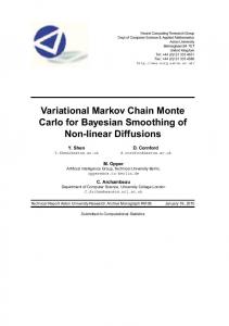
gave a perfect fit to the posterior distributions for both types of parameter estimates . Posterior distributions obtained with the full likelihood were similar to their pseudolikelihood-generated counterparts and also appeared to be perfect gamma-distributions, although they were based on an order of magnitude smaller number of MCMC iterations and therefore were not as smooth (see Figure 1A-D). The main use of the posterior distributions in our applications is for determining

Pacific Symposium on Biocomputing 6:203-214 (2001)

the maximum posterior-probability estimates of parameters (each estimate of this kind corresponds to the mode of a marginal posterior distribution) and for inferring the maximum posterior density confidence intervals. Both inferences can be done with far greater precision when results of MCMC computations are fitted to an analytically defined density function (see Figure 1E). This is especially important for the inference of confidence intervals, because in the absence of an analytical function an accurate analysis of the tails of posterior distributions requires an enormous number of MCMC iterations.

(A)

(B)

Average error of estimation of confidence intervals (for upper bound, Vk dataset).

(E) Error

MCMC estimation

Gamma approximation

Number of iterations

(C)

(D)

(F)

47

Figure 1. Full likelihood MCMC-estimated marginal posterior density functions (shown with continuous lines) (A and B) for relative rate variation parameters and C and D for the branch-length parameters. The dotted lines show the fitted gamma-densities functions. (E) Average error of estimation of maximum posterior density confidence intervals with (dotted line) and without (solid line) gamma-density approximation. Gamma-approximation significantly improved the precision of the estimates for the same number of MCMC iterations. (F) Distribution of wavelet parameter number in model selection with pseudolikelihood function; 19,000 MCMC iterations were used for computing this distribution.

6.4. Model selection The MCMC program designed for model selection behaved in a similar way with all analyzed datasets. We describe in detail only the analysis of immunoglobulin κ

Pacific Symposium on Biocomputing 6:203-214 (2001)

sequences. Pseudolikelihood-based MCMC iteration started with a large number of model parameters (> 65 - for a set of sequences where only 57 sites were variable!). After about a thousand burn-in iterations, the random walk reached what appeared to be an equilibrium state. The mode of the rate parameter number distribution (see Figure 1F) was equal to 47, which is intuitively a reasonable value. A few thousands more MCMC iterations showed that the average pseudolikelihood slowly increased and that the mode of the rate parameter number distribution moved steadily towards the smaller values. Therefore, we concluded that we are looking at an example of pathologically slow convergence of an MCMC random walk. Full likelihood-based model selection showed similar tendencies - it started with large number of parameters (about 70) that, after approximately 500 iterations, dropped below 57. We were not able to study full likelihood model selection for as many iterations as we completed with the pseudolikelihood version, but we could see that it would take hundreds, if not thousands, of additional iterations for the MCMC random walk to reach equilibrium. Although we are currently unable to prove this conjecture generally, we suspect that the wavelet-model selection with pseudolikelihood-based MCMC gives results similar to those of MCMC model selection with the full likelihood. We expect that the pseudolikelihood version of model selection is slightly more conservative - that is, it favors more parameter-rich models - than the full-likelihood version of the same procedure. We expect it to be more conservative because the pseudolikelihood function corresponds to the assumption that data contain much more information than they do under the full likelihood model. Therefore, we conjecture that it is acceptable to use the pseudolikelihood function for the wavelet-model selection. 6.5. MCMC with jumps among alternative trees. For all datasets that we analyzed with MCMC that involved jumps between phylogenetic trees, the optimal tree was reached surprisingly fast (usually in fewer than 100 MCMC iterations, even when the starting tree was different from the optimum tree at every partition). After reaching the optimum tree, the MCMC process was always trapped there permanently. There must exist datasets that contain little information about the correct tree, however; for them, the MCMC process should switch indecisively among alternative trees until the end of simulation.) Therefore, the results that we obtained earlier (1) using MCMC with a fixed (optimum) tree should be identical to the results obtained with full MCMC.

7. Conclusion We developed and implemented a new computational tool that raises our hopes that

Pacific Symposium on Biocomputing 6:203-214 (2001)

we can make useful the wavelet model of rate variation. Although we displayed an apparent obsession with the analysis of proteins in this study, the method presented here is also applicable to evaluation of rate variation in nucleotide sequences. In the future we could modify the model-selection routine to include reversible jumps from a wavelet model to a gamma-model (15) and back. Such jumps should make possible model selection in a more general framework. The exercises that we performed in this study with the wavelet model should be completely reproducible with a Fourier model (1), although the computational price would be higher due to the non-local nature of the discrete Fourier decomposition. The statistical comparison of rate variations in two homologous protein subfamilies appears to have been almost completely overlooked (one exception is Gu’s method (16)) by other published mathematical approaches. Thus, our algorithm is an important addition to the current arsenal of research tools in genomics and evolutionary biology. 8. References 1. Morozov, P., Sitnikova, T., Churchill, G., Ayala, F. J. & Rzhetsky, A. (2000) Genetics 154, 381-395. 2. Durbin, R., Eddy, E., Krogh, A. & Mitchison, G. (1998) Biological Sequence Analysis. (Cambridge University Press, Cambridge). 3. Golding, G. B. (1983) Mol Biol Evol 1, 125-142. 4. Yang, Z., Goldman, N. & Friday, A. E. (1995) Systematic Biology 44, 384-399. 5. Felsenstein, J. (1981) J Mol Evol 17, 368-376. 6. Tavare, S. (1986) Lectures in Mathematics in the Life Sciences 17, 57-86. 7. Daubechies, I. (1988) Wavelets (S.I.A.M., Philadelphia). 8. Metropolis, S. C., Rosenbluth, A., Rosenbluth, M., Teller, A. & Teller, E. (1953) J Chem Phys 21, 1087-1092. 9. Hastings, W. K. (1970) Biometrika 57, 97-109. 10. Kirkpatrick, S., Gelatt, C. D. & Vecchi, M. P. (1983) Science 220, 671-680. 11. Gilks, W. R., Richardson, S. & Spiegelhalter, D. J. (1996), (Chapman & Hall/ CRC, New York). 12. Zuckerkandl, E. & Pauling, L. (1965) in Evolving Genes and Proteins, eds. Bryson, V. & Vogel, H. J. (Academic Press, New York), pp. 97-166. 13. Mau, R., Newton, M.A., & Larget, B. (1996) Technical Report #961. Department of Statistics, University of Wisconsin at-Madison, Madison, OH. 14. Green, P. J. (1994), (Dept. of Matematics, University of Bristol., Bristol, Geat Britain). 15. Yang, Z. (1993) Mol Biol Evol 10, 1396-1402. 16. Gu, X. (1999) Mol Biol Evol 16, 1664-1674.