Markov Decision Processes for Optimizing Human Workflows

Espinosa, Frausto, and Rivera: Markov Decision Processes for Optimizing Human Workflows Service Science 2(4), pp. 245-269, © 2010 SSG

Markov Decision Processes for Optimizing Human Workflows Enrique D. Espinosa University of Waterloo 295 Hagey Blvd., Suite 240, Waterloo, Ontario, Canada, N2L 6R5 [email protected]

Juan Frausto Instituto Tecnológico y de Estudios Superiores de Monterrey Campus Cuernavaca Autopista del Sol km. 104, Colonia Real del Puente, Xochitepec, Morelos, México, 62790 [email protected]

Ernesto J. Rivera Instituto Tecnológico y de Estudios Superiores de Monterrey Campus Cuernavaca Autopista del Sol km. 104, Colonia Real del Puente, Xochitepec, Morelos, México, 62790 [email protected]

W

orkflows are used by domain analysts as a tool to describe the synchronization of activities in a business domain. The Business Process Management Notation (BPMN) has become a standard to characterize Workflows. Nevertheless, BPMN alone does not provide tools for aligning business models and IT architectures. Currently, there is not a method which promotes making decisions based on a technique with a probabilistic basis for providing financial value to a [human] workflow. If such method could exist, it would help the domain analyst to understand what sections of the business and IT architecture could be re-engineered for adding value. Markov Decision Processes (MDP’s) can be the centerpiece of such a method. MDP’s are introduced as a means to pinpoint assets to be designed, managed, and continuously improved, while enhancing business agility and operational performance.

Key words: workflow; human workflow; optimization; business process; BPMN; Markov; decision making History: Received Feb. 5, 2010; Received in revised form Apr. 26, 2010; Accepted Apr. 27, 2010; Online first publication Sept. 07, 2010

1. Introduction A Workflow can be defined as a collection of ordered activities to accomplish some business process (Georgakopoulos et al 1995). It is a tool to integrate the supply chain, and it can act as a bridge between two or more organizations (Cardoso et al 2004). It involves “the movement of documents and tasks through a automated work process in order to achieve certain goals” (Tsai et al 2007). Workflows help to model the behavior of diverse processes, characterized as a sequence of activities. Therefore they can be seen as a decision-making problemsolver, where material plus human and machine resources should be optimized. Workflows were used to model supply chains all throughout the 20th century. However, the formal name “workflow” was coined in 1985 at Filenet, a provider of Enterprise Content Management and Business Process Management solutions. Domain Analysts model business units using a process-oriented approach, which can be expressed by a ubiquitous description language. Business Process Management Notation (BPMN) (OMG 2008, White 2004, Ouyang et al 2006) has become a common representational device for this purpose. Nevertheless, the alignment between business objectives and IT architectures is still hard to achieve. BPMN per se cannot model goals, objectives, strategies or tactics (common assets in business models). Added value is a desired item on any enterprise architecture, but it is typically hard to devise by IT staff. Structured methods for finding 245


value, such as balanced scorecards, aren’t still widely used (Malinverno and Hill 2007). In any BPM project, management needs a clear idea of what performance element will improve as a result of the BPM effort (Rosser 2007). For this to happen, strategies must be filtered down as goals of the marketing, development, R&D operations, IT organization and IT infrastructure. Most of the organizations have already detected these operational inefficiencies and are taking aware of process modeling in order to get certain level of Maturity in BPM (Melenovsky 2006). IT would help that humans be a part of the assessment, that is, human workflows appear in the overall design. Assessing the impact of human behavior on the overall business model, based on a probabilistic method could provide a financial benefit, since it would make use of statistical data to support decision-making. In order to optimize business processes, several efforts have been done from different areas: Business Process Management (BPM), Business Intelligence (BI) and Business Rules (BR) have already done approaches to the desired optimization. Nevertheless Forrester Research Inc strongly suggests the combination of the adequate foundations from these three areas in order to find a definitive solution to this challenge (Evelson et al 2008). Markov Decision Processes (MDP’s) are commonly used in BI as a tool for Decision Support and have been widely used to model systems which require decision making. For example, they are used in queue theory for evaluating performance, and for improving system operation while optimizing its performance (Hillier and Lieberman 2004). In this paper, we propose modeling business processes using BPMN Workflows and MDP’s. The goal is to provide mathematical support to decisions in which human behavior plays a role. These decisions are often made in an empirical fashion. In contrast, a method for computing the maximum net gain obtained from the evaluation of employee’s performance is introduced. Based on these calculations, several workflows can be executed until the optimum is obtained. Therefore, time and money can be saved by applying this model. Section two gives a general view about relevant works involved with this field of study. Section three presents the proposal of modeling Workflows with MDPs. Section four shows the results of some preliminary implementations comparing the efficiency of workflows analyzed by MDP’s. Section Five introduces a second scenario in order to test the method with different data. Finally, section six gives an overview for future work and section seven presents the conclusions.

2. Related Work Several research teams have aimed at improving workflows through MDP’s. Doshi et.al. (2004) present an approach to a model for launching Web Services based on policies. Through this work, researchers try to build an “abstract workflow” avoiding implementation details. The authors associate a quality index to each workflow in order to select the best one. This approach leads to a specific objective: they select a Web Service through the use of MDP’s, in order to make the workflow orchestration faster and more efficient (Estublier and Anlaville 2005, Shing 2006, Digiampietri et al 2005). An orchestration is defined as “an executable business process from the perspective and under the control of one single end-point” (Shing 2006). This endingpoint coordinates Web Services in order to define the business process (Digiampietri et al 2005). Magnani and Montesi report (Magnani and Montesi 2007) that they can associate a “cost” to the elements of BPMN notation, which allows them to apply Markov Decision Processes in order to obtain a policy based on the total minimum computed cost of executing a business process. From this angle, they try to implement a mechanism which allows them to choose the workflow that implies the minimum computational cost. This process can be linked with the general mechanism for the execution of the workflow. Van der Aalst and Van Hee (2002) have also applied Markov techniques in order to establish what the chances are of a case taking a particular route through a process. In this sense, the developed models by the aforementioned authors try to evaluate the best workflow in terms of computational effort (or cost) and efficiency and help to choose the “fastest” workflow. In order to accomplish this objective, they [generally] assign certain cost of execution to each of the elements of the workflow. Later, when they have different alternatives for execution, they apply MDP’s in order to obtain the actions’ sequence (i.e. policy) which allows them to choose the shortest workflow among a group of candidates (Doshi et al 2004, Magnani et al 2007). These investigations attempt to minimize the computational cost of workflow execution. In the other hand, a new approach of obtaining Workflow by an MDP which seeks to minimize the financial cost of executing an entire workflow is proposed in this paper. In our research, we optimize the workflow design in order to obtain a financial advantage, based on human behavior and/or capacities. 246


The proposed contribution focuses in providing a strategic boost to the enactment of a workflow that includes MDP’s. Its components can be differentiated by exhibiting different levels of performance and different maintenance costs. An action will be defined as the execution of a task under the constraint imposed by their own differentiation. As an example, in a stock exchange transaction, a task (e.g. a stock quotation) may be executed by a rookie, or we can hire a more specialized professional with a higher academic level and experience. Similarly, the job may be assigned to two assistant brokers, or perhaps one assistant broker plus one specialized staff. This will result in different costs of execution, due to the salary gap between diverse employee profiles, as well as in different performance effectively solving tasks, not to mention quality discrepancies among them. The strategic challenge is to choose the form of execution which gives the best cost/benefit ratio. The decision will be probabilistic, as output by executing an MDP.

3. Modeling MDP’s + BPMN As mentioned before, BPMN is a notation used for representing workflows in a graphical way. BPMN gives a view of workflows presumably understood by business and IT professionals alike. An example of this notation is presented on Figure 1. This workflow represents the process to be enacted by a stock exchange broker. The process starts when the stock exchange issues quotes. The bids reach the brokers on the trading floor. The broker calculates the future market value based on the opening price, volume and statistical data. The auction session then starts. Once the stockholder decides which shares to acquire, he notifies the broker, who in turn makes an offer to the auction. If he is successful, then he is awarded the stock. The notification and purchased titles are transferred to the stockholder. Witness Figure 1. BPMN consists of symbols that represent the different elements (processes, states, decisions, resources, etc.). The Boolean operator XOR does not include a mechanism for taking the best action for the decision. Besides, the current modeling technique does not have a mechanism to optimize resources. Figure 2 is a fragment from Figure 1. In it, there is only one way to execute the task: use a “default” staff selection , which may have been overlooked at this point in the Domain Analysis (for this example, we assume that the staff includes only one assistant). Nevertheless, people with different profiles could be hired in order to quote the stocks: then a new possibility could be added: to hire a new person with a higher degree of competence. This would presumably optimize the “quote stocks” process. Whether this actually triggers a decision, at this moment three (or more) possible actions can be taken: a) To execute the process with a default staff (one assistant). b) To hire a new broker with more capabilities (higher profile). c) To hire a new broker and one more assistant. There is a significant difference between an assistant and a broker: the broker will have more formal studies (for example a college degree). As a consequence, he will have more competences and will be able to handle larger responsibilities. Because of this, he will receive a higher salary with respect to the assistant option. This may be a drawback on operation costs, especially if these added skills may be spared from the process. His assets would also be larger: a better capacity for finishing his tasks, which will result in more stock quotes per day. So, which is the better staff selection? A basis and a mechanism are needed to make the decision. The proposed mechanism is a Markov Decision Processes (MDP) driven by a human workflow. We represent the MDP as an addition to the current BPMN notation without drastically changing it. Meanwhile, the MDP representation could be graphically seen as the addition of a sub-process with the legend “[MDP]” included in the name. Inside the sub-process specification, a flow split with a distinctive icon with two arrows ( ) pinpointing different roads to take as shown on Figures 3 and 4.

247


Figure 1 BPMN Workflow for a Stock Exchange

Figure 2. Fragment of the Workflow: Quoting Stocks

248


Figure 3 New BPMN Diagram with MDP Sub-process Specification

Figure 4 MDP Sub-process Specification with Added Flow Split and Proposed Notation

In order to use an MDP, it is necessary to provide it with information like transition probabilities and the cost/reward matrix. The information needed to supply to the MDP can be found in a well known, but not fully utilized, administrative tool: the Balanced Scorecard (Kaplan and Norton 1996). The Scorecard provides a measurement tool for staff performance. It allows to see what would the difference in performance be (plus the resulting economical benefit/cost) between employees with different profiles. A simple Scorecard looks similar to Figure 5. It is the basis for obtaining the aforementioned information after a mapping process. Figure 5 shows two different profile evaluations: current staff and broker skills. Three main skills are characterized: formal studies, competences and responsibilities. A weight is given, to estimate the impact of each skill in the overall qualification. Column punctuation shows the skill performance level for the described profile. For this example, levels are given according to the next scale: 1 = poor 2 = marginal 3 = average 4 = good 5 = excellent Figure 5 An Example of a Simple Scorecard Actor #1 Profile: stock exchange staff member current Weight Punctuation Formal studies 0.4 2 Competences 0.4 3 Responsibilities 0.2 3 Total Score Base salary Weighted salary

Score broker 0.8 1.2 0.6 2.6

$ 12,500.00

Weight Punctuation Score 0.4 4 1.6 0.4 4 1.6 0.2 3 0.6 3.8 $ 12,500.00

$ 12,825.00

$ 12,975.00

249


Punctuation describes an employee’s performance level. As bigger the number is, better the performance is. Finally a score is calculated for each skill by multiplying weight and punctuation columns. The scores are summed and the result is multiplied by the base salary in order to obtain a weighted salary, according to the skills levels. As a first step, the Markovian states are determined. This is an intuitive process which requires a sound analysis. For the example above, the markovian states are set according to the quantity of stock quotes the staff may produce in a given mainframe: • • •

Low quotation capacity Average quotation capacity High quotation capacity

Next, we need to represent a transit schema between Markovian States. For this purpose, we use a Transition Matrix. In MDP’s, a Transition Matrix is calculated based on statistical data. Its structure is obtained from the Scorecard. The transition probabilities for each of the states are thus obtained. For this example some values have been mapped from the Balanced Scorecard and have been used in order to propose a method for their conversion to probabilistic values. It is necessary to establish “ideal values”. These ideal values are the expected values for the current employees’ performance. In other words, they are the quantity of stocks quoted in a day for the different productivity levels. For this example, 15 Stocks Quoted (SQ) have been assigned for low performance level; 50 SQ for the average performance level and 90 SQ for high performance level as ideal values. Then the [real] number of quotes that the employees quote in a day is obtained. It is assumed that the employee has [actually] quoted 16 Stocks per Day (SPD) while having a low performance, 24 SPD while having an average performance and 32 SPD while having a high performance. Next, the difference between the ideal values and the real values for each performance level of the different profiles is calculated. Following the example, when the employee makes a transition from low performance to high performance, the difference between the ideal and the real (90-16=74) is obtained. Once the calculations are made, the values shown on Table 1 are obtained. Values are normalized for a percentile probability. The procedure is explained next. The absolute value for the numbers on each obtained row is added. For the case ‘low’, the result is 109. Now each absolute value is substracted to the previously calculated sum (109-1=108, 10934=75, 109-74=35). Results are shown on Table 2.

Table 1 Differences Between Ideal and Real Values for State ‘low’ Case1: Low

Low

Average -1

High 34

74

Table 2 Preprocessed Values Low Low

Average 108

High 75

35

Finally, the preprocessed values are converted to percentile probability. Percentile probability is obtained by summing the values in the corresponding row, and then each cell’s value is divided by the obtained sum. For example the percentile value for cell (low, low) is 108/(108+75+35)=0.4954. The final value is then rounded to 0.5 for easy handling. The final Transition Matrix with values formatted to probabilities for this example is shown on Table 3.

250


Table 3 Example Transition Action 1: Current Staff Action: Current staff Low

Avg

High

0.50

Low

0.34

0.16

Average

Low

High

Action 3: hire 1 broker & 1

Action 2: hire 1 broker Action: Hire 1 broker Low

Low

Low

0.35

Avg

High

0.44

0.21

Average

Action: Hire 1 broker assistant & 1 assistant

High Low

Low

Avg Low High Average

0.25

0.46

Low

0.50 Average

0.34 0.46

0.16 0.17 Low Average 0.35 0.37 0.25

Low0.19 0.460.44 0.29 0.21 Average

Average

0.46High

0.41 0.37

0.40 High 0.17 0.19 Average

0.330.46 0.49

High

0.41

0.40

0.18 0.25

0.19 High

0.18

0.33

HighAverage 0.25 0.29

0.49 High

0.29

High

0.25 0.45 0.36

0.46

0.29

0.33 0.19 0.42

0.36

0.45

0.33

0.42

0.25

The Cost/reward matrix (See Table 4) is calculated based on the differential between financial revenue provided by each of the proposed actions. In turn, this differential is provided by strategic alignment with company goals using scorecards. The Balanced Scorecard provides weights given to individual competences as referred to by the [personal] evaluation of his credentials. In order to obtain these data, it is necessary to calculate the time per unit (of work) that each type of employee needs for completing the task while having a low, average and high productivity. Cost per day is then obtained, as long as the net income. The difference between cost and income gives the net gain. The difference between net gains of the states is then placed in the cost/reward matrix at the corresponding state transition. This calculus is realized because the change from one state to other implies the need of calculate the difference between the obtained gain at the different cases. Values for this matrix are divided by 1,000,000 [Mexican pesos (MXN)]. Once all the necessary data for the Markov Decision Process have been determined, one of the methods for solving MDP’s: complete enumeration, dynamic programming, policy iteration, etc. Besides, it is possible to plan at a finite or infinite horizon. Table 4 Example Cost/Reward Action 1: Current Action:Staff Current staff Low Low

Low

Average 0

Low

0 Average

Average

-0.48High

High

-0.96

0.48 -0.48 -0.96 0

-0.48

Avg

High 0.48

Low

High 0.96

0.96 Low 0 0.48 -0.48 0.48

Action 3: hire 1 broker & 1

Action 2: Hire hire1 1broker broker Action: Low

0 High

High

Low 0 Average High 0.96 3.12

Average

High 0 Average

Avg

Action: Hire 1 broker & 1 assistantassistant

0 -0.96

-3.12 -0.96

-3.12

Low Low

0

Low-1.44 0 0.962.16 3.12 Average -2.16

00

-2.16

-4.08 2.16HighAverage

0

High

Avg Low

High Average

1.44

4.08

0

0 2.64

-2.64 -1.44 0

-4.08

High

1.44

4.08

0

2.64

-2.64

0

For this problem we have experimented with all the available techniques for solving MDP’s. We have found that some techniques perform better than others. Results about it are shown on Section 4. The next step is to implement a DSS using the Markovian Transition and Cost/Reward Matrixes, in order to allow decision making (with MDP support) while modeling BPMN Workflows.

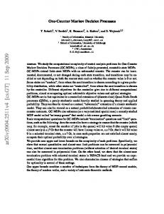
4. Implementing the Markov Decision Process We now introduce software solutions for solving MDP’s applied to business process, using several markovian techniques. These applications are programmed in Java. The algorithms are implemented following specific methodologies. In order to evaluate their relevance for optimizing the employee’s performance, the example in Section 3 has been used. The comparison parameter is the quality of the solution. It was measured comparing the reward (maximum income) calculated through the MDP methods. The higher value obtained is taken as a reference. A graph for this parameter is shown at figure 6. Some abbreviators have been used: CE-F is the equivalent for Complete Enumeration for Finite horizon, DP-F is the abbreviation for Dynamic Programming for Finite horizon, CE-I, PI-I, PID-I are the equivalent for Complete Enumeration, Politic Iteration and Politic Iteration with Discount factor.

251


Figure 6. Maximum Income Obtained with MDP Methods

Maximum income 7 x 1,000,000 pesos

6 5 4 3 2 1 0 CE-F

DP-F

CE-I

PI-I

PID-I

The method that presented a higher maximum income is Policy Iteration with Discount Factor for infinite horizon. On the other hand, Complete Enumeration for infinite horizon predicted the lower income. Notice that these methods have been provided with the information about [efficiency] benefit and cost (Table 4), as long as the probabilities for state change (Table 3). These data describe the individual performance (and cost) of each employee. As a consequence the MDP methods select the best action sequence to optimize benefits, getting the maximum income based on data from the Balanced Scorecard (Figure 5). Providing these data, the best policy for each possible decision is obtained. Figure 7 Dynamic Programming Algorithm Inputs: actions, policies_numb, m, trans_mat, costRew_mat, epochs Begin k=1, i=1 do vi=accumulateIncome(trans_mat, costRew_mat) k++ while(k0) i-while(i>0) End Outputs: fn, optimal_policy

The DP algorithm (see figure 7) delivers the expected optimum income (fn) and the optimal policy for finite horizon. The algorithm first calculates the vi vector which contains the cumulative income. Then the Bellman Equation (1) is recursively applied in order to obtain the optimal policy and the expected optimum income (Hillier and Lieberman 2004, Taha 2007, Winston 2004). m

f n (i ) = máx{v + ∑ pijk f n+1 ( j )} k

k i

(1)

j =1

252


The algorithm for Policy Iteration with discount factor (PID) is shown on figure 8. It turned out to be the best method for solving MDP’s with finite horizon in small BPMN workflows. Figure 8 Policy Iteration Algorithm Inputs: actions, policies_numb, m, trans_mat, costRew_mat, discount_factor Begin k=random_select_policy() do vi=accumulateIncomeFor Policy(trans_mat, costRew_mat, po) π=iterationEquations(trans_mat, discount_factor, po) m

f (i ) = v ik + ∑ p ijk f ( j ) j =1

newPolicy=obtainPolicy(fn) while(newPolicy!=k) optimal_policy=newPolicy End Outputs: expected_optimum_income,

A random policy ‘k’ is chosen by PID algorithm. Then the accumulate income vector (vi) for the selected policy is calculated (Taha 2007). This method needs (but we don’t know them) the transition probabilities for the state n, so it is necessary to calculate them. Because of that reason, it calculates the transition probabilities in the equilibrium through the Chapman Kolmogorov equations (Hillier and Lieberman 2004, Taha 2007).

E + f ( policy ) + f ( s ) P s = π s

(2)

Once the transition probabilities in the equilibrium have been determined, policy iteration is performed, based on a modified Bellman equation (3). m

f (i ) = v + ∑ pijk f ( j ) k i

(3)

j =1

Finally the new policy is compared to the policy k. If both policies are not identical, the new policy is selected as the policy k and the process is performed again, else the new policy is declared as the optimal and process is over (Hillier and Lieberman 2004, Taha 2007, Winston 2004). The application of MDP’s to the workflow reflects a more efficient process as long as how obtained policy is applied. The results of the finite horizon algorithm (DP) applied to the example from Section 3 are resumed on Table 5 with an optimum income of 5.468 million MXN. The PID algorithm points out that a broker and an assistant should be hired while the state is low or average. On the other hand, when the state is high, the current staff should be enough. This algorithm determines a maximum income of 5.79 million MXN. Table 5 Results from DP algorithm State

Epoch 1

Epoch 2

Epoch 3

Low Average High

Hire broker & assist. Hire broker & assist. Current staff

Hire broker & assist. Current staff Current staff

Hire broker & assist. Hire broker & assist. Hire broker & assist.

253


The goal of this method comparison is to determine the method with better performance applied to BPM Workflows. Then they can be combined with the proposed model from section 3. This combination allows aligning the MDP for decision making and BPMN for workflow modeling with one of every organization’s objectives: the enterprise growth through a bigger economical benefit (Rosser 2007). In other words, money is saved as much as possible by optimizing the decisions taken through the complete workflow.

5.

A Second Scenario

In order to test the effectiveness of the method, a second scenario has been proposed. Based on the workflow in Figure 1, the fragment shown on figure 9 is focused. This figure shows the initial process in the stockbrokerage. This process starts when a quote is received and it is necessary to calculate the future market value. Another Markov Decision Process has been implemented, since it can help to decide what type of broker to hire, in order to maximize the maximum expected income. Figure 9 Fragment of the Original BPMN workflow

This time it is necessary to know what type of employee will be in charge of calculating the future market value (we will for sure hire him/her). Brokers ready to work with different skills can be found, even with different skills levels. A broker needs according to (HowToAll 2006) four elemental skills: communication, Mathematics skills, Mathematics + statistics skills and Portfolio handling experience. These skills will determine the type of broker is needed to optimize the expected benefit from the transaction, because, as long as they get a different pay, they also have a different level of quality at their evaluations, besides, the different skills can influence the time they need to develop their job. According to this and Section 3, the resulting model for the MDP sub-process can be seen as a four flow division (witness figure 10). The reason for this division is that an employee who has all the four skills (probably at different level [determined by the MDP]) is required. In order to find the adequate profile, four Markovian Processes will be built (one for each skill). In order to implement the MDP’s we need to obtain certain data that help us to make the different matrixes needed for the Markovian Process. First we need again to work with the Balanced Scorecard (see Section 2). At this part of the process, we need to take a look at the Scorecard for this employee, shown on figure 11.

254


Figure 10 MDP added to the Original BPMN Workflow

Figure 11 Balanced Scorecard for Broker in Stockbrokerage Profile: stockbrokerage staff member skill Weight Communication Math skills Math+statistics Portfolio handling experience Total Score Base salary

0.3 0.2 0.4 0.1

$

12,500.00

The necessary skills for a broker can be seen at the Scorecard (figure 11), as long as the weight of each of them for the profile. Also a table (derived from the scorecard book) can be calculated showing the cost related to each of these skills. In other words, it is necessary to know how expensive is to obtain each skill in an employee. For this example, tables shown on figure 12 have been built.

255


Figure 12 Costs of the Different Skill Levels. Cost Proactivity High Medium Low Cost Proactivity High Medium Low

Communication Good Average Low 0.6 0.3 0.3 0.4 0.1 0.3 Mathematics skills Good Average Low 0.6 0.3 0.3 0.4 0.1 0.3

0.1 0.3 0.1

0.1 0.3 0.1

Cost Proactivity High Medium Low Cost Proactivity High Medium Low

Mathematics + statistics skills Good Average Low 0.6 0.3 0.1 0.3 0.4 0.3 0.1 0.3 0.1 Portfolio handling experience Good Average Low 0.45 0.45 0.1 0.28 0.4 0.32 0.27 0.15 0.58

These tables show the relation between the skill level and its impact over the final employee performance, as long as the cost of this relation. At these tables a value closer to one, means a higher pay. On the other hand, a value closer to zero means a lower pay. Besides, it is necessary to obtain other values in order to determine the cost/reward matrix. These values include the cost of the stock (c) (a cost of 50,000 MXN Pesos is supposed) and an estimated profit (p) from buying the stock. This profit has been estimated in three scenarios: good, average and low. These scenarios are directly related with the degree of confidence that the broker exhibits when making quotes to the client (which can also be high, medium and low). It is also needed to know the base salary (b) and the weight (w) of the analyzed skill. These last two values are easily obtained from the Scorecard for the employee’s profile (see figure 11). It is necessary to remember that one MDP for each employee’s skill is going to be designed. As a consequence four different transition matrixes and four different cost/reward matrixes are built. The states of the MDP correspond to the performance of the broker. For this example high, medium and low [performance] states have been stated. In order to obtain all the positions of each cost/reward matrix (M), skills costs (S) tables are used (witness figure 12), applying the equation (4).

M ij = ( pa − ( Sij * b * w + c)) / factor

(4)

Where: • • • • • • • •

M=Cost/reward matrix S = Skill cost matrix i, j = matrixes indexes pa = profit in the corresponding scenario b =base salary w = skill weight c =cost of the stock factor= factor to make it easier calculus (1000)

Finally transition matrixes are built. Once more, these transition matrixes should be based on statistical data about the performance of the employee based on the different skills. The transition matrixes for the Markovian Process corresponding to the communication skill are shown on table 6. The corresponding cost/reward matrixes are shown on table 7. Tables 8 and 9 show the transition matrixes as long as cost/reward matrixes for Mathematics skill. Tables 10 and 11 show the corresponding matrixes for Math+statistics skill. Finally, tables 12 and 13 show the skill ‘portfolio handling experience’. Table 6 Transition Matrixes for Communication Skill Action 2: Hire an average Action 1: Hire a good communication communication broker broker High Medium Low High Medium Low High 0.6 0.3 0.1 High 0.55 0.3 Medium 0.3 0.65 0.05 Medium 0.25 0.4 Low 0.1 0.1 0.8 Low 0.05 0.3

256

Action 3: Hire a low communication broker High Medium Low 0.15 High 0.2 0.4 0.4 0.35 Medium 0.1 0.3 0.6 0.65 Low 0.01 0.09 0.9


Once necessary data have been obtained, software tools are used, in order to solve the MDP’s, as described in Section 4. As a result the more beneficial policy is obtained. This policy states the type of employee to hire. Again, we have experimented by running the Decision Process for finite horizon with 3 stages and infinite horizon. Table 7 Cost/Reward Matrixes for Communication Skill Action 3: Hire a low communication Action 2: Hire an average Action 1: Hire a good communication broker communication broker broker High Medium Low High Medium Low High Medium Low High 12.25 -11.125 -10.375 17.75 18.875 19.625 High 47.75 48.875 49.625 High -11.125 -11.5 -11.125 18.875 18.5 18.875 Medium Medium 48.875 48.5 48.875 Medium -10.375 -11.125 -10.375 19.625 18.875 19.625 Low Low 49.625 48.875 49.625 Low

Table 8 Transition Matrixes for Mathematics Skills Action 1: Hire a good Mathematics skills broker

High High Medium Low

Medium Low 0.44 0.33 0.32 0.54 0.24 0.34

Action 2: Hire an average Mathematics skills broker

High 0.23High 0.14Medium 0.42Low

Action 3: Hire a low Mathematics skills broker

High

Medium Low 0.51 0.38 0.35 0.35 0.08 0.27

0.11 High 0.3 Medium 0.65 Low

Medium Low 0.2 0.42 0.1 0.27 0.24 0.38

0.38 0.63 0.38

Table 9 Cost/Reward matrixes for Mathematics Skills Action 1: Hire a good Mathematics skills broker


48.5 49.25 49.75

Action 2: Hire an average Mathematics skills broker

Action 3: Hire a low Mathematics skills broker

Medium Low High Medium Low High Medium Low - 11.5 - 10.75 - 10.25 49.25 49.75 High 18.5 19.25 19.75 High - 10.75 - 11 - 10.75 49 49.25 Medium 19.25 19 19.25 Medium - 10.25 - 10.75 - 10.25 49.25 49.75 Low 19.75 19.25 19.75 Low

Table 10 Transition Matrixes for Math+Statistics Skills Action 1: Hire a good Mathematics + statistics skills broker

High Medium Low

High

Medium Low 0.9 0.09 0.8 0.1 0.35 0.34

Action 2: Hire an average Mathematics + statistics skills broker

0.01High 0.1 Medium 0.31Low

High

0.49 0.35 0.08

Medium Low 0.5 0.5 0.55

Action 3: Hire a low Mathematics + statistics skills broker

High 0.01 High 0.15 Medium 0.37 Low

0.2 0.1 0.05

Medium Low 0.4 0.5 0.55

0.4 0.4 0.4

Table 11 Cost/Reward Matrixes for Math+Statistics Skills Action 1: Hire a good Mathematics + statistics skills broker


47 48.5 49.5

Action 2: Hire an average Mathematics + statistics skills broker

Action 3: Hire a low Mathematics + statistics skills broker

High Medium Low Medium Low High Medium Low - 13 - 11.5 17 18.5 19.5 High 48.5 49.5 High - 11.5 - 12 18.5 18 18.5 Medium 48 48.5 Medium - 10.5 - 11.5 19.5 18.5 19.5 Low 48.5 49.5 Low

- 10.5 - 11.5 - 10.5

Table 12 Transition Matrixes for Portfolio Handling Experience Skill Action 1: Hire a good Portofolio handling

Action 2: Hire an average Portofolio

Action 3: Hire a low Portofolio handling

handling skills broker skills broker skills broker High Medium Low High Medium Low High Medium Low High 0.9 0.09 0.01 High 0.49 0.5 0.01 High 0.2 0.4 Medium 0.8 0.1 0.1 Medium 0.35 0.5 0.15 Medium 0.1 0.5 Low 0.35 0.34 0.31 Low 0.08 0.55 0.37 Low 0.05 0.55

257

0.4 0.4 0.4


Table 13 Cost/Reward Matrixes for Portfolio Handling Experience Action 1: Hire a good Portofolio handling skills broker

High Medium Low

Action 2: Hire an average Portofolio handling skills broker

Action 3: Hire a low Portofolio handling skills broker

High Medium Low High Medium Low High Medium Low - 10.5625 - 10.5625 - 10.125 49.4375 49.4375 49.875 High 19.4375 19.4375 19.875 High - 10.35 - 10.5 - 10.4 49.65 49.5 49.6 Medium 19.65 19.5 19.6 Medium - 10.3375 - 10.1875 - 10.725 49.6625 49.8125 49.275 Low 19.6625 19.8125 19.275 Low

The resulting policy is resumed on table 14. Notice that obtained policy with infinite horizon is exactly the same than that obtained with finite horizon and it recommends hiring an employee good at the four necessary skills. The maximum expected income obtained in the finite horizon is resumed in the graphic at figure 13. From these results can concluded that (because of the low ratio in the cost/proactivity) it is necessary to hire a good employee in all the skills, but we can have a bigger profit if we don’t give him too many responsibilities, if he has a low performance his salary will decrease helping to have a big margin of profit. By the way, the results from infinite horizon (see figure 14), confirm the same tendency, showing similar curves to those obtained in finite horizon. The new conclusion from these last results is that while longer time planning; the bigger profit can be obtained. Table 14 Resulting Policy from the MDP for Finite Horizon and Infinite Com munication State Stage 1 Stage 2 Stage 3 H igh Good Goo d Go od Average Good Goo d Go od L ow Good Goo d Go od Mathematics+statistics skills State Stage 1 Stage 2 Stage 3 High Go od Good Goo d Average Go od Good Goo d Lo w Go od Good Goo d

Mathematics skills State Stage 1 Stage 2 Stage 3 High Go od G ood Good Average Go od G ood Good Low Go od G ood Good Portf olio h andling experience State Stage 1 Stage 2 Stage 3 High Goo d G ood G ood Average Goo d G ood G ood Low Goo d G ood G ood

It can be noticed at these results a singular phenomenon. From the policy obtained, it can be seen a tendency to hire an “ideal employee”. This is because the data used on this case are based on experimental data. The same example has been tested, using variations of the data, which results in different policies and expected values. The mentioned variations include a bigger base salary for the employee and a smaller future stock value (smaller profit); besides variations to the transition matrixes have been made. Resulting profiles and expected values are shown next. Figure 13 Maximum Expected Income Obtained with Finite Horizon 50 49 Communication 48

x1,000

Mathematics skill 47 46

Math+statistics skill

45

Portfolio handling experience

44 High

Average

Low

258


Figure 14 Maximum Expected Income Obtained with Infinite Horizon

175

x1,000

170 165

Communication

160

Mathematics skills

155

Mathematics+stat istics skills

150


145 140 High

Average

Low

The first variation consisted in a reduced future stock value. This reduction, impacted directly in a smaller profit, reflected in the cost/reward matrixes. The resulting profile for finite horizon in three stages is shown on Table 15. The new maximum expected income is shown at figure 15. Same data for infinite horizon are resumed on table 16 and figure 16. Table 15 Resulting Policy from the First Data Variation, Finite Horizon Communication State Stage 1 Stage 2 High Average Average Average Average Average Low Good Good State High Average Low

Mathematics+statistics skills Stage 1 Stage 2 Stage 3 Stage 3 State Average Average Average Average High Average Average Average Average Good Low Good Good Good Good

Mathematics skills Stage 1 Stage 2 Stage 3 Good Good Good Good Good Good Good Good Good

Portfolio handling experience State Stage 1 Stage 2 Stage 3 High Good Good Good Average Good Good Good Low Good Good Good

Table 16 Resulting Policy for First Data Variation, Infinite Horizon

State

Communication Mathematics

Statistics

Experience

High

Average

Good

Average

Good

Average

Average

Good

Average

Good

Low

Good

Good

Good

Good

259


Figure 15 Maximum Net Income for First Data Variation, Finite Horizon

Max. Net Income (x1,000)

14 13 Communication

12

Mathematics skill

11

Math+statistics skill

10


9 8 High

Average

Low

Performance

From these figures can be noticed that a more flexible profile has been obtained, varying the employees’ skill level between average and good. Nevertheless the maximum net income is reduced in these data. This reduction is because of the future value of the stock, which is lower than the initial one; giving a minor profit from the stock purchase. This profit reduction is more drastically reflected when results for infinite horizon are compared, which has been reduced from values between 155 000 and 175 000 to values between 11 000 and 14 000. Figure 16 Maximum Net Income for First Data Variation, Infinite Horizon

17

Max. Net Income (x1,000)

16 15

Communication

14 Mathematics skills

13 12

Mathematics+statisti cs skills

11


10 High

Average

Low

Performance

A second data variation was made in order to see if it showed a different behavior: it included a small increment to the employees’ base salary. Besides, transition probabilities were modified, giving bigger transition possibilities to the medium performance state. The obtained policy for finite horizon (witness table 17) showed a more balanced profile, having an average level at mathematics skill. On the other hand portfolio handling experience didn’t show any variation at all. The policy for Infinite horizon showed exactly the same than first data variation (see table 16). Besides, the maximum net income (see figures 17 and 18) resulted also with similar values and curves if compared to the first data variation.

260


Table 17 Resulting Policy for Second Data Variation, Finite Horizon

Communication Mathematics+statistics skills Stage 1 Stage 2 Stage 3 State Stage 1 Stage 2 Stage 3 Average Average Average High Average Average Average Average Average Average Average Average Average Average Good Good Good Low Good Good Good Portfolio handling experience Mathematics skills Stage 1 Stage 2 Stage 3 State Stage 1 Stage 2 Stage 3 State Good Good Good High Average Average Average High Average Good Good Good Average Average Average Good Good Good Good Low Good Good Good Low State High Average Low

x1,000 Max. Net Income (x1000)

Figure 17 Maximum Net Income for Second Data Variation, Finite Horizon

14 13 Communication 12 Mathematics skill 11 Math+statistics skill

10


9 8 High

Average

Low

Figure 18 Maximum Net Income for Second Data Variation, Infinite Horizon

Max. Netx1,000 Income (x1000)

16 15 14

Communication

13

Mathematics skills

12

Mathematics+stat istics skills

11


10 9 High

Average

Low

The analyzed case is valid for demonstration purpose. Nevertheless, it is not designed strictly according to the reality. For example, in the reality usually there are more than 3 employee profiles. In order to show a more realistic 261


view of this case, a last case has been run, involving a variation: five skill levels have been introduced (Expert, Competent, Medium, Marginal and Low) replacing the three previous levels (High, Medium and Low). These skill levels represent five different actions (policies). The Markovian Process must choose one among these policies for every system state.

Table 18 Transition Matrixes for Five Policies Case, Communication Skill Action 1: Hire an expert communication skill broker

Action 3: Hire a medium communication skill broker

Action 2: Hire a competent communication skill broker

High

Average

High

0.6

0.3

Low 0.1 High

High

Average

0.55

0.3

Average

0.3

0.6

0.1 Average

0.25

Low

0.1

0.1

0.8 Low

0.05

Action 4: Hire a marginal communication skill broker

Low

High

Average

Low

0.15 High

0.7

0.2

0.1

0.4

0.35 Average

0.6

0.2

0.2

0.3

0.65 Low

0.5

0.3

0.2

Action 5: Hire a low communication skill broker

High

Average

High

0.4

0.3

Low 0.3 High

Average

0.2

0.4

0.4 Average

Low

0.1

0.4

0.5 Low

High

Average

Low

0.2

0.4

0.4

0.1

0.3

0.6

0.01

0.09

0.9

Table 19 Cost/Reward Matrixes for Five Policies Case, Communication Skill Action 2: Hire a competent communication skill broker

Action 1: Hire an expert communication skill broker High High Average Low

Average

20

19

19.7

19

High

Low 29.5 High

24.875

25.625 18.4 19.9 Low Action 4: Hire a marginal communication skill broker

17.1

High

High

Average

Low

12.4

11.2

13.9

13.3 24.5 24.875 Average 12.5 24.875 25.625 Low Action 5: Hire a low communication skill broker

10.1

12

12

11.3

Average

23.75

21 Average

High

Average

9.75

9.875

Average

8.875

9.5

Low

9.625

9.875

Action 3: Hire a medium communication skill broker

24.875

Low 9.625 High

Low 25.625 High

High

Average

Low

-3.25

-1.125

-0.375

9.875 Average

-2.125

-1.5

-1.125

9.625 Low

-1.375

-1.125

-0.375

262


Table 21 Cost/Reward Matrixes for Five Policies Case, Mathematics Skill

Table 20 Transition Matrixes for Five Policies Case, Mathematics Skill

Action 2: Hire a competent mathematics skill broker

Action 1: Hire an expert mathematics skill broker High

Action 1: Hire an expert mathematics skill broker

Average Low

High

Average

Low

High

0.6

0.3

0.55

0.3

0.15

High

Average

0.3

0.6

0.1 Average

0.25

0.4

0.35

Average

25.25

Low

0.1

0.1

0.8 Low

0.05

0.3

0.65

Low

24.75

0.1 High

Action 3: Hire a medium mathematics skill broker High

High

High

0.7

0.1 High

Average

0.6

0.2

0.2 Average

0.2

Low

0.5

0.3

0.2 Low

0.1

0.4

Average Low

Average Low

Average 19.1 22.4

0.3

0.4

0.4

Average

22.2

0.4

0.5

Low

25.5

High

Average

Low

-1.5

-0.75

-0.25

Average

-0.75

-1

-0.75

Low

-0.25

-0.75

-0.25

Action 2: Hire a competent math + statistics skill broker

Table 23 Cost/Reward Matrixes for Five Policies Case, Math + Statistics skill

Action 1: Hire an expert math + statistics skill broker

High

Average

Low

0.55

0.3

0.15

High

0.25

0.4

0.35

Average

38.7

39

0.05

0.3

0.65

Low

35.1

37.4

Action 4: Hire a marginal math + statistics skill broker

High

Average

40

38

High

Average

Low

0.1 High

0.4

0.3

0.3

High

0.2

0.2 Average

0.2

0.4

0.4

0.1 0.3 0.2 Low Action 5: Hire a low math + statistics skill broker

0.4

0.5

High

Average

25.4

22.2

Average

27.3

21.1

Low

25.5

Action 2: Hire a competent math + statistics skill broker

Low

High Average

39.5 High 41 Average 39.9 Low

Action 3: Hire a medium math + statistics skill broker

0.2

Low

11.1

0.6

Average Low

Average

13.9

13

0.9

Action 3: Hire a medium math + statistics skill broker

High

9.9

0.3

0.1 Average 0.8 Low

0.6

10.9 25 25.14 Low 12.3 Action 5: Hire a low mathematics skill broker

0.09

0.6

0.5

Low

0.1

0.3

Low

Action 4: Hire a marginal mathematics skill broker

0.01

Average

Average

11.25 10.75

13.1

High

0.3

0.7

9 10.25

11.3

0.4

0.6

High

9.25 10.75

Average

Low

High

High

12.75

13.4

0.4

0.1 High

0.1

Low

9.25

High

Average

Average Low

0.1

Average

8.5

Low

0.2

Action 1: Hire an expert math + statistics skill broker

Low

High

24.7 High 23.7 Average

High

Table 22 Transition Matrixes for Five Policies Case, Math + Statistics Skill

High

25 23.23 Average 22.25 20.75 Low

21.2

Action 5: Hire a low mathematics skill broker High

Low

25.5 19.75 High

High High

0.3

Average

24.5

Action 3: Hire a medium mathematics skill broker

Action 4: Hire a marginal mathematics skill broker

Average Low 0.2

High

Action 2: Hire a competent mathematics skill broker

47.75

Low 49.625

48.875

48.5

48.875

49.625

48.875

49.625

Action 4: Hire a marginal math + statistics skill broker High Average

Low 26.9 High 24 Average

17.75

18.875

Low 19.625

18.875

18.5

18.875

24 23.3 Low 19.625 Action 5: Hire a low math + statistics skill broker

18.875

19.625

High

Average

Low

0.2

0.4

0.4

High

High Average -12.25

Low

-11.125 -10.375

0.1

0.3

0.6

Average

-11.125

-11.5 -11.125

0.01

0.09

0.9

Low

-10.375

-11.125 -10.375

263

48.875


Table 24 Transition Matrixes for Five Policies Case, Portfolio Handling Experience

High

Action 3: Hire a medium portfolio handling experience skill broker

Action 2: Hire a competent portfolio handling experience skill broker

Action 1: Hire an expert portfolio handling experience skill broker High

Average

High

Average

High

Average

Low

0.3

0.4

0.3 High

0.2

0.6

0.2 High

0.25

0.35

0.4

0.5

0.4 Average

0.1

0.5

0.4 Average

0.35

0.45

0.2

0.5

0.3 Low

0.2

0.4

0.4 Low

0.5

0.45

0.05

Average

0.1

Low

0.2

Low

Action 5: Hire a low portfolio handling experience skill broker

Action 4: Hire a marginal portfolio handling experience skill broker High

High

Average

0.3

0.4

Low

Low 0.3 High

High

Average

Low

0.3

0.4

0.3

Average

0.2

0.3

0.5 Average

0.2

0.3

0.5

Low

0.2

0.4

0.4 Low

0.2

0.4

0.4

Table 25 Cost/Reward Matrixes for Five Policies Case, Portfolio Handling Experience Action 1: Hire an expert portfolio handling experience skill broker High

Average

Action 2: Hire a competent portfolio handling experience skill broker

Low

High

Average

14.8 High

Action 3: Hire a medium portfolio handling experience skill broker

Low

High

Average

Low

14.1

14.1

14.0

13.8

14.8 High

13.64

13.64

13.92

Average

14.44

14.2

14.36 Average

14.3

14.2

14.5 Average

13.776

13.68

13.744

Low

14.46

14.7

13.84 Low

14.5

14.7

15.0 Low

13.784

13.88

13.536

High

Action 4: Hire a marginal portfolio handling experience skill broker

Action 5: Hire a low portfolio handling experience skill broker

High

Average

Low

High

Average

Low

High

14.0

14.5

14.4 High

Average

15.0

14.5

14.7 Average

-0.112

-0.18

-0.18

-0.16 -0.128

-0.04

Low

14.9

14.1

14.9 Low

-0.108

-0.06 -0.232

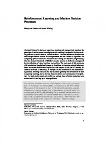
For this case five matrixes are needed for the markovian process. Markovian matrixes for four skills are shown from Table 18 to Table 25. These values were obtained again based on the experience of the authors. Once the matrixes have been designed, the Markovian Process is performed. Resulting policy of the MDP is shown on Table 26. Maximum Net Income is shown on Figure 19.

Table 26 Resulting Policy for All Skills, Five Policies Case State

Communication skill State

High

Competent

High

Mathematics skill Expert

Average Competent

Average Expert

Low

Competent

Low

State

Math + statistics skill

State

High

Medium


High

Marginal

Average

Medium

Average

Marginal

Low

Competent

Low

Competent

264

Expert


Figure 19 Maximum Net Income for Five Policies Case 90

Max. Net Income (x1000)

80 Communication 70

Mathematics

60

Math+statistics

50


40 High

Average

Low

Performance

From this experiment a different behavior in the policy can be seen, as long as in the different curves on Figure 19. This behavior is caused because the values in the corresponding matrixes have more weight in different actions than in the first experiments. This has provoked the difference in the curves and the difference in the policies, which look more varied. In this figure, in general terms, a bigger profit could be obtained if an average state in mathematics skills is reached and maintained. In similar way, an average state of performance in portfolio handling experience is recommended to achieve and maintain. According to the curves in Figure 19, a bigger profit can be obtained if a low performance in communication and statistics is achieved; this last asseveration is caused possibly because of the salaries increment or other factors [costs] that affect the profit and losses. The behavior shown in the different scenarios leaves to an important conclusion: When a Markovian process for Decision making in BP is modeled, it is necessary to get as grained data as possible, in order to make a more accurate prediction. Besides, it is quite important to get data from adequate sources (such as the Balanced Scorecard). In this sense, the most trustable the source is, the most adequate the resulting policy is.

6.

Further work

Further work consists on the design of larger cases, including a complete organization structure and Business Process. The addition of historical data to the MDP model is proposed, in order to make the design strictly according to reality. The resulting policy from MDP’s improves the performance of our BPMN Workflow in different ways. In the particular case previously analysed, the time required for quote stocks is minimized. Figure 20 is a fragment of the Workflow corresponding to the Stockbrokerage (Sections 3 and 4) modified accordingly to the “five policies case” (Section 5) shown on Figure 10. Figure 20 details the communication skill, showing the MDP application for selection between five skill levels. Figure 20 Communication Skill Decision Trough MDP in BPMN

265


Figure 21 BPMN Workflow Including MDP Modeling and Characterization

The modification or addition to the notation including the MDP impact is not the main focus of this paper, but it will be addressed in future works. As a preview it is possible to visualize the decision taken and its consequences in an added scheme to the process model (See Figure 21). Figure 21 shows an important addition: the proposed icon for MDP representation in BPMN ( ), this icon was discussed on Section 3. Not only graphical notation should be addressed but the BPMN xml schema (Ouyang et al 2006) should be modified also. BPMN xml schema is used to save the diagrams in an xml formatted file. A preliminary proposal could look as shown in Figure 22. This xml document includes a fragment of a possible schema for including Markov Decision Process information for the skill “Communication” in the “five policies case” (Section 5). We have outlined in bold the new proposed section for MDP modeling. These last proposals are merely approaches needing further development and they are placed here only to show the possible direction of our research. Once the business process has been modeled in BPMN notation, it is necessary to translate this notation to the execution language BPEL. Some efforts have already been done such as (Asztalos et al 2009, García-Bañuelos 2009, Mazanek & Minas 2009, Ouyang et al 2006). Nevertheless, according to our research, we need to figure a way to include the impact of the MDP execution, with the selection of the best options for profiles and skill selection. Then, the MDP results should be included as task assignments in the XML that defines the BPEL process. Finally, the possible implementation of a tool capable of joining the classic modeling technique for Business Process with the Markovian model introduced in this paper is being currently developed. This development would result in a tool capable of decision making for business process execution improvement. Besides it could be possible to identify optimization parameters and to elaborate an execution report.

7.

Conclusions

It has been introduced a new application for Markov Decision Processes in the field of Business Processes Management. A general method for modeling the elements for a Markov Decision Process from different elements commonly used in Business Process Management has been described. This paper proposes a method for Decision Support based on observable data (Markov Decision Processes propose a policy based on the analysis of these data). A different approach to those described on previous sections (see Section 2) has been made. Through this method BPMN can give an extra economical profit to most organizations, as long as the inclusion of the human performance in the workflow modeling. In this approach foundations from Business Process Management (BPM) and Business Intelligence (BI) have been combined in order to optimize Workflows (Evelson et al 2008).

266


Figure 22 A Possible Modification to the BPMN XML Schema for Saving and Characterizing Markov Decision Processes and Their Result and Impact over the Model … … … … … …

267


About Markov Decision Processes, through this research, the performance of different methods for solving MDP’s providing BPMN Workflows a mechanism for decision making while optimizing different resources. As long as MDP’s are divided by horizon (finite and infinite) it has been found that the best MDP method for solving BPMN workflows with finite horizon is Dynamic programming, while Policy Iteration with Discount Factor is the best for infinite horizon. Besides, different scenarios while having data variations have been tested in order to feed with different data the MDP, then the behavior shown for the decision making on each case has been analyzed. From these modifications to the case of study, it has been seen how some differences in the matrixes make a different prediction in the resulting policy, as long as a visible difference in the predicted maximum net income. Because of this, we strongly suggest to be careful when obtaining statistical, historical data about people’s performance (Scorecard Book) and their influence over the final workflow and the decisions taken with the Markovian Processes, in order to make more exact predictions when this method is applied in real scenarios. From these experiments can be concluded that a more fine-grained design of the Markovian states observed on the process flow and a good method for data collection will result in a trustable policy. References Asztalos, M., T. Mészáros, L. Lengyel (2009), “Generating Executable BPEL Code from BPMN Models”. Unpublished. http://is.tm.tue.nl/staff/pvgorp/events/grabats2009/submissions/grabats2009_submission_16final.pdf. (Last accessed on October 14, 2009). Cardoso, J., R. Bostrom, A. Sheth (2004), ”Workflow Management Systems and ERP Systems: Differences, Commonalities and Applications”. Information Technology and Management. Vol. 1, No. 3-4. pp 319-338. Digiampietri, L. A., C. B. Medeiros, J. C. Setubal (2005), “A framework based on Web service orchestration for bioinformatics workflow management”. Genetics and Molecular Research. Vol. 3, No. 4. pp. 535-542. Doshi, P., K. Verna, R. Goodwin, R Akkiraju (2004), “Dynamic Workflow Composition using Markov Decision Processes”. Proceedings of the IEEE International Conference in Web Services (ICWS ’04). pp 576-582. Estublier, J. and S. Anlaville (2005), “Business Process and Workflow Coordination of Web Services”. Proceedings of the IEEE International Conference on e-Technology, e-Commerce and e-Service, 2005. pp. 85-88. Evelson, B., C. Teubner and J. Rymer (2008). “How The Convergence Of Business Rules, BPM and BI Will Drive Business Optimization”. Forrester Research, Inc. May 14, 2008. García-Bañuelos, L. (2009). “Translating BPMN Models to BPEL Code”. Unpublished. http://is.tm.tue.nl/staff/pvgorp/events/grabats2009/submissions/grabats2009_submission_22banuelos.pdf. (Last accessed on October 14, 2009). Georgakopoulos, D., Hornick, M. and Sheth, A.. (1995). “An Overview of Workflow Management: From Process Modeling to Workflow Automation Infrastructure”. Distributed and Parallel Databases. Vol. 3, No. 2. pp 119153. Hillier, F. and G. Lieberman (2004), Introduction to Operations Research, Mc Graw Hill, New York, USA. HowToAll, (2006) “How to become a stockbroker”. http://www.howtoall.com/Educationfiles/ Howtoallbecomestockbroker.htm. (Last accessed on April 10, 2008). Kaplan, R. S. and D. P. Norton (1996), The Balanced Scorecard: Translating Strategy into Action. Harvard Business School Press. 322 p. USA. Magnani, M. and D. Montesi (2007), “Computing the cost of BPMN diagrams”. Technical Report UBLCS-07-17. University of Bologna. Italy. Malinverno, P. and J. B. Hill. (2007), “SOA and BPM Are Better Together”. Gartner Research. ID Number: G00145586. Mazanek, S. and M. Minas. (2009), “Transforming BPMN to BPEL Using Parsing and Attribute Evaluation with Respect to a Hypergraph Grammar”. Online: http://is.tm.tue.nl/staff/pvgorp/events/grabats2009 /submissions/grabats2009_submission_8.pdf. (Last accessed on October 14, 2009). Melenovsky, M. J. and J. Sinur (2006). BPM Maturity Model Identifies Six Phases for Successful BPM Adoption. Gartner Research. ID Number: G00142643. OMG, Object Management Group (2008), “Business Process Modeling Notation, V1.1: OMG Available Specification”. http://www.bpmn.org/Documents/BPMN 1-1 Specification.pdf. (Last accessed on April 29, 2009). Ouyang, C., M. Dumas, A. Hofstede, W.M.P. Van der Aalst (2006), “From BPMN Process Models to BPEL Web Services”. IEEE International Conference on Web Services, 2006. pp. 285 – 292. 268


Rosser, B. (2007), “How to Achieve BPM Alginment With Enterprise Goals”. Gartner Research. ID Number: G00152759. Shing, S. (2006) “BPEL: Building Standards-Based Business Processes with Web Services”. Online course. http://www.javapassion.com/webservices/BPELOverview.pdf. Last accessed on March 2, 2009. Taha, H. A. (2007), Operations Research: An introduction. Pearson-Prentice Hall. Upper Saddle River, N.J. USA. Tsai, C.H., H.J. Luo, F.J. Wang (2007), “Constructing a BPMN Environment with BPMN*”. Proceedings of the 11th IEEE International Workshop on Future Trends of Distributed Computing Systems (FTDCS’07). pp 164-172. Van der Aalst, W. M. P. and K. Van Hee (2002). Workflow Management: Models, Methods and Systems. MIT Press. Cambridge, Mass., USA. White, S.A. (2004), “Introduction to BPMN”. IBM Corporation. http://www.bpmn.org/Documents/ Introduction to BPMN.pdf. (Last accessed on April 29, 2009). Winston, W. L. (2004), Operations Research: applications and algorithms. Thomson Brooks/Cole. Belmont, CA. USA. Enrique D. Espinosa, Ph.D., received a Bachelor of Science in Computer Science (1987) from the University of Kansas, a Master of Science in Computer Science (1991) and a Ph.D. in Computer Science (1998) from the Monterrey Institute of Technology. He currently is a visiting academic at the Center for Business, Entrepreneurship and Technology (CBET) of the University of Waterloo. His research interests include Artificial Intelligence for Services Engineering, Electronic Commerce, and e-Learning.

Juan Frausto, Ph.D., holds a Bachelor of Electrical Engineering (1974) from the Mexican National Polytechnic Institute and he received a Ph.D. on Investigation of Computing Methods in Electrical Engineering (1981) from the Mexican National Polytechnic Institute. He has directed more than 80 M.Sc. and Ph.D. Thesis. He has also published more than 100 articles on international congresses and journals (http://campus.cva.itesm.mx/juanfrausto). Among his publications, Petri Nets, Markov Decision Processes, Lineal Optimization, Simulated Annealing, Neural Networks, Decision Trees and Genetic Algorithms can be found. His research interests include Combining Optimization applied to Artificial Intelligence for Engineering, Bioinformatics, Planning and Scheduling.

Ernesto J. Rivera, M.S.C.S., received a Bachelor of Science in Computer Science (2004) from the State University of Veracruz, Mexico and a Master of Science in Computer Science (2006) from the Monterrey Institute of Technology. Currently he is a Ph.D. candidate at the Monterrey Institute of Technology. His research interests include Services Engineering and Advanced Internet Development.

269

Markov Decision Processes for Optimizing Human Workflows

Markov Decision Processes for Optimizing Human Workflows

Suggest Documents

Markov Decision Processes

Optimizing Quantiles in Preference-based Markov Decision Processes

One-Counter Markov Decision Processes

Characterizing Markov Decision Processes - CiteSeerX

markov decision processes lodewijk kallenberg

INTRODUCTION TO MARKOV DECISION PROCESSES

Variance-penalized Markov decision processes

Learning Qualitative Markov Decision Processes

Fixed Points for Markov Decision Processes - TUM

Factored Partially Observable Markov Decision Processes for ...

Compositional reasoning for Markov decision processes - CiteSeerX

Permissive Supervisor Synthesis for Markov Decision Processes ...

Partially Observable Markov Decision Processes ... - Semantic Scholar

Bayesian learning of noisy Markov decision processes

Hard Constrained Semi-Markov Decision Processes

An Introduction to Markov Decision Processes

Reinforcement Learning and Markov Decision Processes

Reinforcement Learning and Markov Decision Processes

Bounded Parameter Markov Decision Processes with ... - CiteSeerX

"Markov Decision Processes", by Lodewijk Kallenberg

Average-Reward Decentralized Markov Decision Processes - IJCAI

Transition-Independent Decentralized Markov Decision Processes

semi-markov decision processes - Semantic Scholar

Action-Constrained Markov Decision Processes With ...