Markov Decision Processes with Applications to Finance - CiteSeerX

Markov Decision Processes with Applications to Finance

Markov Decision Processes with Applications to Finance ¨ Nicole Bauerle KIT

Jena, March 2011

Markov Decision Processes with Applications to Finance

Outline

I

Markov Decision Processes with Finite Time Horizon I I I

I

Markov Decision Processes with Infinite Time Horizon I I I

I

Definition Basic Results Financial Applications Definition Basic Results Financial Applications

Extensions and Related Problems

Markov Decision Processes with Applications to Finance MDPs with Finite Time Horizon

Markov Decision Processes (MDPs): Motivation Let (Xn ) be a Markov process (in discrete time) with I

state space E,

I

transition kernel Qn (·|x).


Markov Decision Processes (MDPs): Motivation Let (Xn ) be a Markov process (in discrete time) with I

state space E,

I

transition kernel Qn (·|x).

Let (Xn ) be a controlled Markov process with I

state space E, action space A,

I

admissible state-action pairs Dn ⊂ E × A,

I

transition kernel Qn (·|x, a).

A decision An at time n is in general σ(X1 , . . . , Xn )-measurable. However, Markovian structure implies An = fn (Xn ) is sufficient.


MDPs: Formal Definition Definition A Markov Decision Model with planning horizon N ∈ N consists of a set of data (E, A, Dn , Qn , rn , gN ) with the following meaning for n = 0, 1, . . . , N − 1: • E is the state space, • A is the action space, • Dn ⊂ E × A admissible state-action combinations at time n, • Qn (·|x, a) stochastic transition kernel at time n, • rn : Dn → R one-stage reward at time n, • gN : E → R terminal reward at time N.


Policies

I

A decision rule at time n is a measurable mapping fn : E → A such that fn (x) ∈ Dn (x) for all x ∈ E.

I

A policy is given by π = (f0 , f1 , . . . , fN−1 ) a sequence of decision rules.


Optimization Problem For n = 0, 1, . . . , N, π = (f0 , . . . , fN−1 ) define the value functions Vnπ (x) := IEπnx

"N−1 X

# rk Xk , fk (Xk ) + gN (XN ) ,

k=n

Vn (x) := sup Vnπ (x),

x ∈ E.

π

A policy π is called optimal if V0π (x) = V0 (x) for all x ∈ E.


Optimization Problem For n = 0, 1, . . . , N, π = (f0 , . . . , fN−1 ) define the value functions Vnπ (x) := IEπnx

"N−1 X

# rk Xk , fk (Xk ) + gN (XN ) ,

k=n

Vn (x) := sup Vnπ (x),

x ∈ E.

π

A policy π is called optimal if V0π (x) = V0 (x) for all x ∈ E.

Integrability Assumption (AN ): For n = 0, 1, . . . , N sup IEπnx π

"N−1 X k=n

# rk+ (Xk , fk (Xk )) + gN+ (XN ) < ∞,

x ∈ E.


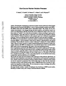
General evolution of a Markov Decision Process

Controller

state at stage n: xn

random transition with reward at stage n: rn(xn,an)

distribution Qn(.|xn,an)

state at stage n+1: xn+1


Literature - Textbooks on MDPs I

Shapley (1953)

I

Bellman (1957, Reprint 2003)

I

Howard (1960)

I

Bertsekas and Shreve (1978)

I I

Puterman (1994) ´ Hernandez-Lerma and Lasserre (1996)

I

Bertsekas (2001, 2005)

I

Feinberg and Shwartz (2002)

I

Powell (2007)

I

B and Rieder (2011)


Notation Let M(E) := {v : E → [−∞, ∞) | v is measurable} and define the following operators for v ∈ M(E):

Definition a) (Ln v )(x, a) := rn (x, a) +

R

v (x 0 )Qn (dx 0 |x, a), (x, a) ∈ Dn ,

b) (Tnf v )(x) := (Ln v )(x, f (x)), x ∈ E, c) (Tn v )(x) := supa∈Dn (x) (Ln v )(x, a). Note Tn v ∈ / M(E). A decision rule fn is called maximizer of v at time n if Tnfn v = Tn v .


Theorem (Reward Iteration) For a policy π = (f0 , . . . , fN−1 ) and n = 0, 1, . . . , N − 1: a) VNπ = gN and Vnπ = Tnfn Vn+1,π , b) Vnπ = Tnfn . . . TN−1fN−1 gN .


Theorem (Reward Iteration) For a policy π = (f0 , . . . , fN−1 ) and n = 0, 1, . . . , N − 1: a) VNπ = gN and Vnπ = Tnfn Vn+1,π , b) Vnπ = Tnfn . . . TN−1fN−1 gN .

Theorem (Verification Theorem) Let (vn ) ⊂ M(E) be a solution of the Bellman equation: vn = Tn vn+1 , vN = gN . Then it holds: a) vn ≥ Vn for n = 0, 1, . . . , N. b) If fn∗ is a maximizer of vn+1 for n = 0, 1, . . . , N − 1, then ∗ vn = Vn and π ∗ = (f0∗ , f1∗ , . . . , fN−1 ) is optimal.


Structure Assumption (SAN ): There exist sets Mn ⊂ M(E) and sets ∆n of decision rules such that for all n = 0, 1, . . . , N − 1: (i) gN ∈ MN . (ii) If v ∈ Mn+1 then Tn v is well-defined and Tn v ∈ Mn . (iii) For all v ∈ Mn+1 there exists a maximizer fn of v with fn ∈ ∆n .


Structure Theorem

Theorem Let (SAN ) be satisfied. Then it holds: a) Vn ∈ Mn and (Vn ) satisfies the Bellman equation. b) Vn = Tn Tn+1 . . . TN−1 gN . c) For n = 0, 1, . . . , N − 1 there exist maximizers fn of Vn+1 with fn ∈ ∆n , and every sequence of maximizers fn∗ of Vn+1 ∗ defines an optimal policy (f0∗ , f1∗ , . . . , fN−1 ).


Upper Bounding Functions Definition b : E → R+ is called an upper bounding function if there exist cr , cg , αb ∈ R+ such that for n = 0, 1, . . . , N − 1: (i) rn+ (x, a) ≤ cr b(x), (ii) gN+ (x) ≤ cg b(x), R (iii) b(x 0 )Qn (dx 0 |x, a) ≤ αb b(x).


Upper Bounding Functions Definition b : E → R+ is called an upper bounding function if there exist cr , cg , αb ∈ R+ such that for n = 0, 1, . . . , N − 1: (i) rn+ (x, a) ≤ cr b(x), (ii) gN+ (x) ≤ cg b(x), R (iii) b(x 0 )Qn (dx 0 |x, a) ≤ αb b(x). αb := sup(x,a)∈D

R

b(x 0 )Q(dx 0 |x,a) . b(x)



R

b(x 0 )Q(dx 0 |x,a) . b(x)

Define kv kb := supx∈E

|v (x)| b(x) .



R

b(x 0 )Q(dx 0 |x,a) . b(x)

Define kv kb := supx∈E

|v (x)| b(x) .

IBb := {v ∈ M(E) | kv kb < ∞}, IBb+ := {v ∈ M(E) | kv + kb < ∞}.


Bounding Functions

Definition b : E → R+ is called a bounding function if there exist cr , αb ∈ R+ such that (i) |rn (x, a)| ≤ cr b(x), (ii) |gN (x)| ≤ cg b(x), R (iii) b(x 0 )Q(dx 0 |x, a) ≤ αb b(x).


Example: Consumption-Investment Problem Financial Market: I I

Bond price: Bn = (1 + i)n , Q Stock prices: Snk = S0k nm=1 Ymk ,

We denote Yn := (Yn1 , . . . , Ynd ).

k = 1, . . . , d.


Example: Consumption-Investment Problem Financial Market: I I

Bond price: Bn = (1 + i)n , Q Stock prices: Snk = S0k nm=1 Ymk ,

k = 1, . . . , d.

We denote Yn := (Yn1 , . . . , Ynd ).

Assumptions: I

Y1 , . . . , YN are independent.

I

(FM): There are no arbitrage opportunities.


Example: Consumption-Investment Problem Policies: I

φkn = amount of money invested in stock k at time n, φn = (φ1n , . . . , φdn ) ∈ Rd .

I

φ0n = amount of money invested in the bond at time n.

I

cn = amount of money consumed at time n, cn ≥ 0.


Example: Consumption-Investment Problem Policies: I

φkn = amount of money invested in stock k at time n, φn = (φ1n , . . . , φdn ) ∈ Rd .

I

φ0n = amount of money invested in the bond at time n.

I

cn = amount of money consumed at time n, cn ≥ 0.

Wealth process: c,φ Xn+1 = (1 + i)(Xnc,φ − cn ) + φn · (Yn+1 − (1 + i) · e)

= (1 + i)(Xnc,φ − cn + φn · Rn+1 )


Optimization Problem

Let Uc , Up : R+ → R+ be strictly increasing, strictly concave utility functions. hP i  c,φ N−1  IEx U (c ) + U (X ) → max c n p  n=0 N  (c, φ) = (cn , φn ) is a consumption-investment strategy with    XNc,φ ≥ 0.


MDP Formulation I

E := [0, ∞) where x ∈ E denotes the wealth,

I

A := R+ × Rd where a ∈ Rd is amount of money invested in the risky assets, c ∈ R+ is amount which is consumed,

I

Dn (x) is given by n Dn (x) := (c, a) ∈ A | 0 ≤ c ≤ x and o (1 + i)(x − c + a · Rn+1 ) ∈ E P -a.s. ,

I

Qn (·|x, c, a) := distribution of (1 + i)(x − c + a · Rn+1 ), rn x, c, a := Uc (c),

I

gN (x) := Up (x).

I


Structure Result Note: b(x) = 1 + x is a bounding function for the MDP.

Theorem a) Vn are strictly increasing and strictly concave. b) The value functions can be computed recursively by VN (x) = Up (x), n o Vn (x) = sup Uc (c) + IE Vn+1 (1 + i)(x − c + a · Rn+1 . (c,a)

c) There exist maximizers fn∗ (x) = (cn∗ (x), an∗ (x)) of Vn+1 and ∗ the strategy (f0∗ , f1∗ , . . . , fN−1 ) is optimal.


Power Utility Let us assume Uc (x) = Up (x) = γ1 x γ with 0 < γ < 1.

Theorem a) The value functions are given by Vn (x) = dn x γ , x ≥ 0. b) Optimal consumption is cn∗ (x) = x(γdn )−δ and the optimal amounts which are invested (δ = (1 − γ)−1 ) an∗ (x) = x

(γdn )δ − 1 ∗ αn , (γdn )δ

x ≥0

where αn∗ is the optimal solution of the problem sup IE[(1 + α · Rn+1 )γ ], α∈An

An = {α ∈ Rd : 1 + α · Rn+1 ≥ 0}.


Semicontinuous MDPs Theorem Suppose the MDP has an upper bounding function b and for all n = 0, 1, . . . , N − 1 it holds: (i) Dn (x) is compact and x 7→ Dn (x) is upper semicontinuous (usc), R (ii) (x, a) 7→ v (x 0 )Qn (dx 0 |x, a) is usc for all usc v ∈ IBb+ , (iii) (x, a) 7→ rn (x, a) is usc, (iv) x 7→ gN (x) is usc. Then Mn := {v ∈ IBb+ | v is usc} and ∆n := {fn dec. rule at n} satisfy the Structure Assumption (SAN ). In particular, Vn ∈ Mn ∗ and there exists an optimal policy (f0∗ , . . . , fN−1 ) with fn∗ ∈ ∆n .

Markov Decision Processes with Applications to Finance MDPs with Infinite Time Horizon

MDPs with Infinite Time Horizon Consider a stationary MDP with β ∈ (0, 1], g ≡ 0 and N = ∞. " J∞π (x) :=

IEπx

∞ X

# β r Xk , fk (Xk ) , k

k=0

J∞ (x) := sup J∞π (x),

x ∈ E.

π

Integrability Assumption (A): " δ(x) :=

sup IEπx π

∞ X k=0

k +

β r

# Xk , fk (Xk ) < ∞,

x ∈ E.


Convergence Assumption (C) " lim sup IEπx

n→∞

π

∞ X

βk r +

# Xk , fk (Xk ) = 0,

x ∈ E.

k=n

Assumption (C) implies that the following limits exist: I

limn→∞ Jnπ = J∞π .

I

limn→∞ Jn =: J ≥ J∞ .

J is called limit value function. Note: J 6= J∞ , J∞ ∈ / M(E).


Example: J 6= J∞ (β = 1)

We obtain: J∞ (1) = −1 < 0 = J(1).


Verification Theorem

Tv (x) = sup

Z n o r (x, a) + β v (x 0 )Q(dx 0 |x, a)

a∈D(x)

Theorem Assume (C) and let v ∈ M(E), v ≤ δ be a fixed point of T such that v ≥ J∞ . If f ∗ is a maximizer of v , then v = J∞ and the stationary policy (f ∗ , f ∗ , . . .) is optimal for the infinite-stage Markov Decision Problem.


Structure Assumption (SA) There exists a set M ⊂ M(E) and a set of decision rules ∆ such that: (i) 0 ∈ M. (ii) If v ∈ M then Tv (x) is well-defined and Tv ∈ M. (iii) For all v ∈ M there exists a maximizer f ∈ ∆ of v . (iv) J ∈ M and J = TJ.


Structure Theorem

Theorem Let (C) and (SA) be satisfied. Then it holds: a) J∞ ∈ M, J∞ = TJ∞ and J∞ = J = limn→∞ Jn . b) There exists a maximizer f ∈ ∆ of J∞ , and every maximizer f ∗ of J∞ defines an optimal stationary policy (f ∗ , f ∗ , . . .).


Example: Dividend Pay-Out Let Xn be the risk reserve of an insurance company at time n. We assume that I

Zn = difference between premia and claim sizes in n-th time interval,

I

Z1 , Z2 , . . . are iid, Zn ∈ Z and P(Z1 = k) = qk , k ∈ Z.

I

P(Z1 < 0) > 0 and IE Z + < ∞.

Control: We can pay-out a dividend at each time-point. Xn+1 = Xn − fn (Xn ) + Zn+1 . Let τ := inf{n ∈ N : Xn < 0} be the ruin time point. Aim: Maximize the expected disc. dividend pay-out until τ .


Formulation as an MDP I

E := Z where x ∈ E denotes the risk reserve,

I

A := N0 where a ∈ A is the dividend pay-out,

I

D(x) := {0, 1, . . . , x}, x ≥ 0, and D(x) := {0}, x < 0,

I

Q({y}|x, a) := qy−x+a if x ≥ 0, else Q({y}|x, a) = δxy ,

I

r (x, a) := a,

I

β ∈ (0, 1).

Then for a policy π = (f0 , f1 , . . .) we have J∞π (x) =

IEπx

"τ −1 X k=0

# k

β fk (Xk ) .


First Results Corollary a) The function b(x) = 1 + x, x ≥ 0 and b(x) = 0, x < 0 is a bounding function. (A) is satisfied. b) (C) is satisfied. c) It holds for x ≥ 0 that x+

β IE Z + β IE Z + ≤ J∞ (x) ≤ x + 1 − βq+ 1−β

where q+ := P(Z1 ≥ 0). In particular (SA) is satisfied with M := IBb .


Bellman Equation The Structure Theorem yields that I

limn→∞ Jn = J∞ ,

I

Bellman equation J∞ (x) =

I

max

a∈{0,1,...,x}

∞ n o X a+β J∞ (x − a + k )qk , k=a−x

Every maximizer of J∞ (which obviously exists) defines an optimal stationary policy (f ∗ , f ∗ , . . .).

Let f ∗ be the largest maximizer of J∞ .


Further Properties of J∞ and f ∗

Theorem a) The value function J∞ (x) is increasing. b) It holds that J∞ (x) − J∞ (y ) ≥ x − y, x ≥ y ≥ 0. c) For x ≥ 0 it holds that f ∗ x − f ∗ (x) = 0.


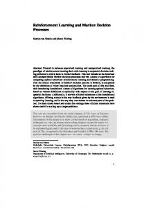
Band and Barrier Policies Definition a) A stationary policy (f , f , . . .) is called band-policy, if ∃ n ∈ N0 and c0 , . . . cn , d1 , . . . dn ∈ N0 s.t. dk − ck−1 ≥ 2, 0 ≤ c0 < d1 ≤ c1 < . . . < dn ≤ cn and  0, if x ≤ c0    x − ck , if ck < x < dk+1 f (x) = 0, if dk ≤ x ≤ ck    x − cn , if x > cn . b) A stationary policy (f , f , . . .) is called barrier-policy if it is a band-policy and c0 = cn .


Band Policies


Barrier Policy


Main Results

Lemma Let ξ := sup{x ∈ N0 | f ∗ (x) = 0}. Then ξ < ∞ and f ∗ (x) = x − ξ

for all x ≥ ξ.

Theorem The stationary policy (f ∗ , f ∗ , . . .) is optimal and a band-policy.


When is the Band a Barrier? Known Condition: P(Z1 ≥ −1) = 1.

I

de Finetti (1957)

I

Shubik and Thomson (1959)

I

Miyasawa (1962)

I

Gerber (1969)

I

Reinhard (1981)

I

Schmidli (2008)

I

Asmussen and Albrecher (2010)


Semicontinuous MDPs Theorem Suppose there exists an upper bounding function b, (C) is satisfied and (i) D(x) is compact for all x ∈ E and x 7→ D(x) is usc, R (ii) (x, a) 7→ v (x 0 )Q(dx 0 |x, a) is usc for all usc v ∈ IBb+ , (iii) (x, a) 7→ r (x, a) is usc. Then it holds: a) J∞ ∈ IBb+ , J∞ = TJ∞ and J∞ = J (Value Iteration). ∗ (x) for all x ∈ E (Policy Iteration). b) ∅ = 6 LsDn∗ (x) ⊂ D∞

c) There exists an f ∗ ∈ F with f ∗ (x) ∈ LsDn∗ (x) for all x ∈ E, and the stationary policy (f ∗ , f ∗ , . . .) is optimal.


Contracting MDP Theorem Let b be a bounding function and βαb < 1. If there exists a closed subset M ⊂ IBb and a set ∆ such that (i) 0 ∈ M, (ii) T : M → M, (iii) for all v ∈ M there exists a maximizer f ∈ ∆ of v , then it holds: a) J∞ ∈ M, J∞ = TJ∞ and J∞ = J. b) J∞ is the unique fixed point of T in M. c) There exists a maximizer f ∈ ∆ of J∞ , and every maximizer f ∗ of J∞ defines an optimal stationary policy (f ∗ , f ∗ , . . .).


Howard’s Policy Improvement Algorithm Let Jf be the value function of the stationary policy (f , f , . . .). Denote D(x, f ) := {a ∈ D(x) | LJf (x, a) > Jf (x)}, x ∈ E.

Theorem Suppose the MDP is contracting. Then it holds: a) If for some subset E0 ⊂ E we define a decision rule h by h(x) ∈ D(x, f ) for x ∈ E0 ,

h(x) := f (x) for x ∈ / E0 ,

then Jh ≥ Jf and Jh (x) > Jf (x) for x ∈ E0 . In this case the decision rule h is called an improvement of f . b) If D(x, f ) = ∅ for all x ∈ E, then the stationary policy (f , f , . . .) is optimal.


Extensions and Related Problems

I

Stopping Problems

I

Partially Observable Markov Decision Processes

I

Piecewise Deterministic Markov Decision Processes

I

Problems with Average Reward

I

Games

Markov Decision Processes with Applications to Finance References

¨ Bauerle, N., Rieder, U. (2011) : Markov Decision Processes with Applications to Finance. Springer. Bellman, R. (1957, 2003): Dynamic Programming. Princeton University Press, NJ. Bertsekas, D.P. and Shreve, S.E. (1978) : Stochastic optimal control. Academic Press, New York. Bertsekas, D.P. (2001,2005) : Dynamic programming and optimal control. Vol. I, II. Athena Scientific, Belmont, MA. Feinberg, E.A. and Shwartz, A. (2002): Handbook of Markov decision processes. Kluwer Academic Publishers, Boston, MA. ´ Hernandez-Lerma, O. and Lasserre, J.B. (1996): Discrete-time Markov control processes. Springer-Verlag, New York.

Markov Decision Processes with Applications to Finance References

Howard, R. (1960) : Dynamic programming and Markov processes. The Technology Press of M.I.T., Cambridge, Mass. Powell, W.B. (2007): Approximate dynamic programming. Wiley-Interscience, Hoboken, NJ. Puterman, M.L. (1994): Markov decision processes: discrete stochastic dynamic programming, John Wiley & Sons, New York. Shapley, L. S. (1953): Stochastic games, Proc. Nat. Acad. Sci., pp. 1095–1100.

Thank you very much for your attention!

Markov Decision Processes with Applications to Finance - CiteSeerX

Markov Decision Processes with Applications to Finance - CiteSeerX

Suggest Documents

Markov Decision Processes with Applications to Finance - Bäuerle ...

Bounded Parameter Markov Decision Processes with ... - CiteSeerX

Characterizing Markov Decision Processes - CiteSeerX

INTRODUCTION TO MARKOV DECISION PROCESSES

Markov Decision Processes with Applications in Wireless ... - arXiv

Markov Decision Processes with Applications in Wireless Sensor - arXiv

Markov Decision Processes

Compositional reasoning for Markov decision processes - CiteSeerX

Action-Constrained Markov Decision Processes With ...

Markov Decision Processes with Functional Rewards - Lip6

An Introduction to Markov Decision Processes

One-Counter Markov Decision Processes

markov decision processes lodewijk kallenberg

Variance-penalized Markov decision processes

Learning Qualitative Markov Decision Processes

Partially Observable Markov Decision Processes ... - Semantic Scholar

Bayesian learning of noisy Markov decision processes

Hard Constrained Semi-Markov Decision Processes

Reinforcement Learning and Markov Decision Processes

Reinforcement Learning and Markov Decision Processes

"Markov Decision Processes", by Lodewijk Kallenberg

Fixed Points for Markov Decision Processes - TUM

Factored Partially Observable Markov Decision Processes for ...

Average-Reward Decentralized Markov Decision Processes - IJCAI