A Markov Logic Network (MLN) is a set of pairs. (F i. , w i. ) where. F i is a formula in first-order logic. w ... A dis
MARKOV LOGIC NASSLLI 2010 Mathias Niepert
MARKOV LOGIC: INTUITION A logical KB is a set of hard constraints on the set of possible worlds Let’s make some of them soft constraints: When a world violates a formula, it becomes less probable, not impossible Give each formula a weight (Higher weight Stronger constraint)
P(world) exp weights of formulas it satisfies
MARKOV LOGIC: DEFINITION
A Markov Logic Network (MLN) is a set of pairs where
(Fi, wi)
Fi is a formula in first-order logic wi is a real-valued weight
Together with a finite set of constants C, it defines a Markov network with One binary node for each grounding of each predicate in the MLN. The value of the node is 1 if the ground atom is true, and 0 otherwise. One feature for each grounding of each formula F in the MLN, with the corresponding weight wi
LOG-LINEAR MODELS
A distribution is a log-linear model over a Markov network H if it is associated with
A set of features F = {f1(D1),…,fk(Dk)}, where each Di is a complete subgraph (clique) of H, A set of weights w1 ,…,wk such that
P (X1; :::Xn) =
1 Z
exp
hP k
i i=1 wi fi (Di )
ASSUMPTIONS 1.
2.
3.
Unique names. Different constants refer to different objects. (Genesereth & Nilsson, 1987) Domain closure. The only objects in the domain are those representable using the constant and function symbols (Genesereth & Nilsson, 1987) Known functions. For each function, the value of that function applied to every possible tuple of arguments is known, and is an element of C
EXAMPLE: FRIENDS & SMOKERS Smoking causes cancer. Friends have similar smoking habits.
EXAMPLE: FRIENDS & SMOKERS Smoking causes cancer. Friends have similar smoking habits.
x Smokes( x) Cancer ( x) x, y Friends ( x, y ) Smokes( x) Smokes( y)
EXAMPLE: FRIENDS & SMOKERS Smoking causes cancer. Friends have similar smoking habits.
1 .5 1 .1
x Smokes( x) Cancer ( x) x, y Friends ( x, y ) Smokes( x) Smokes( y)
EXAMPLE: FRIENDS & SMOKERS Smoking causes cancer. Friends have similar smoking habits.
1.5 x Smokes( x) Cancer ( x) 1.1 x, y Friends ( x, y ) Smokes( x) Smokes( y)
Two constants: Anna (A) and Bob (B)
EXAMPLE: FRIENDS & SMOKERS 1.5 x Smokes( x ) Cancer ( x ) 1.1 x, y Friends ( x, y ) Smokes( x ) Smokes( y )
Two constants: Anna (A) and Bob (B)
Smokes(A)
Cancer(A)
Smokes(B)
Cancer(B)
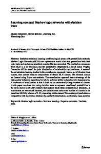
EXAMPLE: FRIENDS & SMOKERS 1.5 x Smokes( x ) Cancer ( x ) 1.1 x, y Friends ( x, y ) Smokes( x ) Smokes( y )
Two constants: Anna (A) and Bob (B) Friends(A,B)
Friends(A,A)
Smokes(A)
Smokes(B)
Cancer(A)
Friends(B,B)
Cancer(B) Friends(B,A)
EXAMPLE: FRIENDS & SMOKERS 1.5 x Smokes( x) Cancer ( x) 1.1 x, y Friends ( x, y ) Smokes( x) Smokes( y)
Two constants: Anna (A) and Bob (B) Friends(A,B)
Friends(A,A)
Smokes(A)
Smokes(B)
Cancer(A)
Friends(B,B)
Cancer(B) Friends(B,A)
EXAMPLE: FRIENDS & SMOKERS 1.5 x Smokes( x ) Cancer ( x ) 1.1 x, y Friends ( x, y ) Smokes( x ) Smokes( y )
Two constants: Anna (A) and Bob (B) Friends(A,B)
Friends(A,A)
Smokes(A)
Smokes(B)
Cancer(A)
Friends(B,B)
Cancer(B) Friends(B,A)
MARKOV LOGIC NETWORKS MLN is template for ground Markov networks Probability of a world x:
1 P( x) exp wi ni ( x) Z i Weight of formula i
No. of true groundings of formula i in x
Typed variables and constants greatly reduce size of ground Markov net Functions, existential quantifiers, etc. Infinite and continuous domains are possible
EXAMPLE: FRIENDS & SMOKERS 1.5 x Smokes( x) Cancer ( x) 1.1 x, y Friends ( x, y ) Smokes( x) Smokes( y)
Two constants: Anna (A) and Bob (B) 1.5 : Smokes( A) Cancer ( A) 1.5 : Smokes( B) Cancer ( B)
1.1 : Friends ( A, A) Smokes( A) Smokes( A) 1.1 : Friends ( A, B) Smokes( A) Smokes( B) 1.1 : Friends ( B, A) Smokes( B) Smokes( A) 1.1 : Friends ( B, B) Smokes( B) Smokes( B)
P( S ( A) T , S ( B) F , F ( A, A) T , F ( A, B) T , F ( B, A) F , F ( B, B) T , C ( A) F , C ( B) T )
1 1 exp wi ni ( x) exp 1.5 *1 1.1* 3 Z i Z
RELATION TO FIRST-ORDER LOGIC Infinite weights First-order logic Satisfiable KB, positive weights Satisfying assignments = Modes of distribution Markov logic allows inconsistencies (contradictions between formulas)
MAP INFERENCE IN MARKOV LOGIC NETWORKS
Problem: Find most likely state of world y given evidence e
arg max P( y | e) y
Query
Evidence
MAP INFERENCE
Problem: Find most likely state of world y given evidence e
1 arg max exp wi ni ( y, e) Ze y i ni is the feature corresponding to formula Fi wi is the weight corresponding to formula Fi
MAP INFERENCE
Problem: Find most likely state of world y given evidence e
arg max wi ni ( y, e) y i ni is the feature corresponding to formula Fi wi is the weight corresponding to formula Fi
MAP INFERENCE 1.5 x Smokes( x ) Cancer ( x ) 1.1 x, y Friends ( x, y ) Smokes( x ) Smokes( y )
Two constants: Anna (A) and Bob (B) Evidence: Friends(A,B), Friends(B,A), Smokes(B) true Friends(A,B) ? Friends(A,A)
Cancer(A)
? Smokes(A)
true Smokes(B)
? Friends(B,A)
true
? Friends(B,B)
Cancer(B)
?
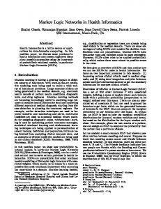
MAP INFERENCE 1.5 x Smokes( x ) Cancer ( x ) 1.1 x, y Friends ( x, y ) Smokes( x ) Smokes( y )
Two constants: Anna (A) and Bob (B) Evidence: Friends(A,B), Friends(B,A), Smokes(B) true Friends(A,B) false Friends(A,A)
Cancer(A)
true Smokes(A)
true Smokes(B)
true Friends(B,A)
true
false Friends(B,B)
Cancer(B)
true
MAP INFERENCE
Problem: Find most likely state of world given evidence e
arg max y
w n ( y, e) i i
i
This is the weighted MAX-SAT problem Use weighted MAX-SAT solver (e.g. MaxWalkSAT) Better: Integer Linear Programming
MAP INFERENCE 1.5 x Smokes( x ) Cancer ( x ) 1.1 x, y Friends ( x, y ) Smokes( x ) Smokes( y )
Two constants: Anna (A) and Bob (B) Evidence: Friends(A,B), Friends(B,A), Smokes(B) :Smokes(A) _ Cancer(A) 1.5 :Smokes(B) _ Cancer(B) 1.5 :Smokes(A) _ Cancer(B) 1.5 :Smokes(B) _ Cancer(A) 1.5 :Friends(A,B) _ :Smokes(A) _ Smokes(B) 0.55 :Friends(A,B) _ :Smokes(B) _ Smokes(A) 0.55 …
RELATION TO STATISTICAL MODELS Special
cases:
Markov networks Bayesian networks Log-linear models Exponential models Max. entropy models Hidden Markov models …
Obtained
by making all predicates zeroarity
Every probability distribution over discrete or finiteprecision numeric variables can be represented as a Markov logic network.
MARKOV LOGIC
Declarative language, several challenges Inference Weight Learning Structure Learning
Many ways to perform probabilistic inference Conditional probability query MAP query
There’s a large body of work on probabilistic inference in graphical models We’ll talk about some of these methods and how they can be put to work in Markov logic networks
INFERENCE IN GRAPHICAL MODELS
Conditional probability queries P(Y|E=e) where Y µX and E µX and Y and E disjoint
P (YjE = e) =
Let W = X – Y – E be the variables that are neither query nor evidence, then
P(y; e) =
P (Y;e) P (e)
P
w P(y; e; w)
P(e) can be computed reusing the previous computation P
P (e) =
y P (y; e)
COMPLEXITY OF INFERENCE The process of “summing out” the joint not satisfactory as it leads to the Exponential blowup that the graphical model representation was supposed to avoid Problem: Exponential blow-up in the worst case is unavoidable Worse: Approximate inference is also NP-hard But: We really care about the cases that we encounter in practice not the worst-case
COMPLEXITY OF INFERENCE Theoretical analysis can focus on Bayesian networks as they can be converted to Markov networks with no increase in representation size First question: How do we encode a BN?
Decision Problem BN-Pr-DP:
DAG structure + worst-case representation of each CPD as a table of size |Val({X_i} [ PaXi )| Given a BN B over X, a variable X 2 X, and a value x 2 Val(X), decide whether PB (X=x) > 0
BN-Pr-DP is NP-complete
COMPLEXITY OF INFERENCE
BN-Pr-DP is in NP: We guess an assignment x to the network variables We check whether X=x holds in x and whether P(x)>0 The latter can be accomplished in linear time using the chain rule of BNs
BN-Pr-DP is NP-hard: Reduction from 3-SAT Given any 3-SAT formula f we can create a Bayesian network B with some distinguished binary variable X such that f is satisfiable if and only if PB(X=x1)>0 The BN has to be constructible in polynomial time
COMPLEXITY OF INFERENCE
For each prop. variable qi one root node Qi with P(qi1)=0.5 For each clause ci one node Ci with edge from Qi to Cj if qi or ¬qi occurs in the clause cj
COMPLEXITY OF INFERENCE
c1 = q1 _ :q3
c10
c11
q10 , q30
0
1
q11 , q30
0
1
q10 , q31
1
0
q11 , q31
0
1
COMPLEXITY OF INFERENCE
We cannot connect the Ci’s (i=1,…,m) directly to the variable X as the CPD for X would be exponentially large We introduce m-2 AND nodes
COMPLEXITY OF INFERENCE
Now, X has value 1 if and only if all of the clauses are satisfied All nodes have at most three parents and, therefore, the size of the BN is polynomial in the size of f
COMPLEXITY OF INFERENCE
Prior probability of each possible assignment is 1/2n P(X=x1) = number of satisfying assignments to f divided by 2n f has a satisfying assignment iff P(x1) > 0
COMPLEXITY OF INFERENCE Probabilistic inference is a numerical problem not a decision problem We can use a similar construction to show the following problem is #P-complete
Given a BN B over X, a variable X 2 X, and a value x 2 Val(X), compute PB (X=x)
We have to do a weighted count of instantiations #P is the set of the counting problems associated with the decision problems in the set NP #P problem must be at least as hard as the corresponding NP problem
COMPLEXITY OF APPROXIMATE INFERENCE Goal is to compute P(Y|e) An estimate r has relative error e for P(y|e) if:
r 1 e
P( y | e) r (1 e )
We can use a similar construction again to show the following problem is NP-hard
Given a BN B over X, a variable X 2 X, and a value x 2 Val(X), find a number r that has relative error e for PB (X=x)
COMPLEXITY OF APPROXIMATE INFERENCE Goal is to compute P(Y|e) An estimate r has absolute error e for P(y|e) if:
| P( y | e) r | e Computing P(X=x) up to some absolute error r has a randomized polynomial time algorithm However, when evidence is introduced, we’re back to NP-hardness Following problem is NP-hard for any e 2 (0,1/2)
Given a BN B over X, a variable X 2 X, a value x 2 Val(X), and an observation E=e, find a number r that has absolute error e for PB (X=x|e)
MONTE CARLO PRINCIPLE ?
Consider the game of solitaire: What’s the probability of winning a game? Hard to compute analytically because winning or losing depends on a complex procedure of reorganizing cards Let’s play a few hands, and see empirically how many do in fact win Idea: Approximate a probability distribution using only samples from that distribution
Lose Lose Lose Win Lose Chance of winning is 1 in 5!
SAMPLING FROM A BAYESIAN NETWORK
Generate samples (particles) from a Bayesian network using a random number generator i0 normal i1 high
d0
easy d1 difficult
g1 A g2 B g3 C
1 1
l0 weak l1 strong 3
s0 low s1 high
SAMPLING FROM A BAYESIAN NETWORK
Generate samples (particles) from a Bayesian network using a random number generator i0 normal i1 high
d0
easy d1 difficult
g1 A g2 B g3 C
1 1
l0 weak l1 strong 3
s0 low s1 high
SAMPLING FROM A BAYESIAN NETWORK
Generate samples (particles) from a Bayesian network using a random number generator i0 normal i1 high
d0
easy d1 difficult
g1 A g2 B g3 C
1 1
l0 weak l1 strong 3
s0 low s1 high
SAMPLING FROM A BAYESIAN NETWORK
Generate samples (particles) from a Bayesian network using a random number generator i0 normal i1 high
d0
easy d1 difficult
g1 A g2 B g3 C
1 1
l0 weak l1 strong 3
s0 low s1 high
SAMPLING FROM A BAYESIAN NETWORK
Generate samples (particles) from a Bayesian network using a random number generator i0 normal i1 high
d0
easy d1 difficult
g1 A g2 B g3 C
1 1
l0 weak l1 strong 3
s0 low s1 high
SAMPLING One sample can be computed in linear time Sampling process generates a set of particles D = {x[1],…,x[M]} When computing P(y), the estimate is simply the fraction of particles in which y “was seen”
P^D =
1 M
PM
m=1 1fy[m]
= yg
with 1 the indicator function and y[m] the assignment to Y in particle x[m]
EXAMPLE: BAYESIAN NETWORK INFERENCE
Suppose we have a Bayesian network with variables X Our state space is the set of all possible assignments of values to variables We can draw a sample in time that is linear in the size of the network Draw N samples, use them to approximate the joint
1st sample: D=d0,I=i1,G=g2,S=s0, L=l1 2nd sample: D=d1,I=i1,G=g1,S=s1, L=l1 …
REJECTION SAMPLING
Suppose we have a Bayesian network with variables X
We wish to condition on some evidence E=e and compute the posterior over Y=X-E
Draw samples and reject them when not compatible with evidence e Inefficient if the evidence is itself improbable we must reject a large number of samples
1st sample: D=d0,I=i1,G=g2,S=s0, L=l1 2nd sample: D=d1,I=i1,G=g1,S=s1, L=l1 …
reject accept
SAMPLING IN MARKOV LOGIC NETWORKS Sampling is performed on the ground Markov logic network Alchemy uses a variant of the MCMC (Markov Chain Monte Carlo) method Can answer arbitrary queries of the form P(Fi|MLNC,L) Example: P(Cancer(Alice)|MLNC,L)
MAP INFERENCE IN GRAPHICAL MODELS
The following problem is NP-complete:
Given a BN B over X and a number t, decide whether there exists an assignment x to X such that P(x) > t.
There exist several algorithms for MAP inference with reasonable performance on most practical problems
MAP INFERENCE IN MARKOV LOGIC NETWORKS
Problem: Find most likely state of world y given evidence e
arg max wi ni ( y, e) y i ni is the feature corresponding to formula Fi wi is the weight corresponding to formula Fi
MAP INFERENCE IN MARKOV LOGIC NETWORKS
Problem: Find most likely state of world given evidence e
arg max y
w n ( y, e) i i
i
This is the weighted MAX-SAT problem Use weighted MAX-SAT solver (e.g. MaxWalkSAT) Better: Integer Linear Programming
THE MAXWALKSAT ALGORITHM for i ← 1 to max-tries do solution = random truth assignment for j ← 1 to max-flips do if ∑ weights(sat. clauses) > threshold then return solution c ← random unsatisfied clause with probability p flip a random variable in c else flip variable in c that maximizes ∑ weights(sat. clauses) return failure, best solution found
MAP INFERENCE IN MARKOV LOGIC NETWORKS We’ve tried Alchemy (and MaxWalkSAT) and the results were poor Better results with integer linear programming (ILP) ILP performs exact inference Works very well on the problems we are concerned with Originated in the field of operations research
LINEAR PROGRAMMING A linear programming problem is the problem of maximizing (or minimizing) a linear function subject to a finite number of linear constraints Standard form of linear programming:
n
maximize
c x j
j 1 n
subject to
a x j 1
ij
xj
j
j
bi
(i
( j 1, 2, ...,
0
1, 2, ..., m) n)
INTEGER LINEAR PROGRAMMING An integer linear programming problem is the problem of maximizing (or minimizing) a linear function subject to a finite number of linear constraints Difference to LP: Variables only allowed to have integer values
n
maximize
c x j
j 1
subject to
n
a x j 1
ij
xj
j
j
bi
(i
( j 1, 2, ...,
0
1, 2, ..., m) n)
x j {...,1,0,1,...} 54
MAP INFERENCE 1.5 x Smokes( x ) Cancer ( x ) 1.1 x, y Friends ( x, y ) Smokes( x ) Smokes( y )
Two constants: Anna (A) and Bob (B) Evidence: Friends(A,B), Friends(B,A), Smokes(B) :Smokes(A) _ Cancer(A) 1.5 :Smokes(B) _ Cancer(B) 1.5 :Smokes(A) _ Cancer(B) 1.5 :Smokes(B) _ Cancer(A) 1.5 :Friends(A,B) _ :Smokes(A) _ Smokes(B) 0.55 :Friends(A,B) _ :Smokes(B) _ Smokes(A) 0.55 …
MAP INFERENCE - EXAMPLE :Smokes(A) _ Cancer(A) 1.5
Introduce new variable for each ground atom: sa , ca Introduce new variable for each formula: xj Add the following three constraints: sa + xj ¸ 1 -ca + xj ¸ 0 -xj - sa + ca ¸ -1 Add 1,5xj to the objective function
n
maximize
c x j 1
subject to
j
j
j
bi
n
a x j 1
ij
x j {0,1}
(i 1, 2, ..., m)
TOMORROW Ontology Matching with Markov Logic Weight Learning Experiments