Online Max-Margin Weight Learning with Markov Logic Networks

Online Max-Margin Weight Learning with Markov Logic Networks Tuyen N. Huynh and Raymond J. Mooney Department of Computer Science The University of Texas at Austin 1 University Station C0500 Austin, Texas 78712-0233, USA {hntuyen,mooney}@cs.utexas.edu Abstract Most of the existing weight-learning algorithms for Markov Logic Networks (MLNs) use batch training which becomes computationally expensive and even infeasible for very large datasets since the training examples may not fit in main memory. To overcome this problem, previous work has used online learning algorithms to learn weights for MLNs. However, this prior work has only applied existing online algorithms, and there is no comprehensive study of online weight learning for MLNs. In this paper, we derive new online algorithms for structured prediction using the primaldual framework, apply them to learn weights for MLNs, and compare against existing online algorithms on two large, real-world datasets. The experimental results show that the new algorithms achieve better accuracy than existing methods.

Introduction Statistical relational learning (SRL) concerns the induction of probabilistic knowledge that supports accurate prediction for multi-relational structured data (Getoor and Taskar 2007). These powerful SRL models have been successfully applied to a variety of real-world problems. However, the power of these models come with a cost, since they can be computationally expensive to train, in particular since most existing SRL learning methods employ batch training where the learner must repeatedly run inference over all training examples in each iteration. Training becomes even more expensive in larger datasets containing thousands of examples, and even infeasible in some cases where there is not enough main memory to fit the training data (Mihalkova and Mooney 2009). A well-known solution to this problem is online learning where the learner sequentially processes one example at a time. In this work, we look at the problem of online weight learning for Markov Logic Networks (MLNs), a recently developed SRL model that generalizes both full first-order logic and Markov networks (Richardson and Domingos 2006). Riedel and Meza-Ruiz (2008) and Mihalkova and Mooney (2009) have used online learning algorithms to learn weights for MLNs. However, previous work only applied one existing online algorithm to MLNs and did c 2010, Association for the Advancement of Artificial Copyright ° Intelligence (www.aaai.org). All rights reserved.

not provide a comparative study of online weight learning for MLNs. In this work, we derive new online algorithms for structured prediction from the primal-dual framework (ShalevShwartz and Singer ; Shalev-Shwartz 2007; Kakade and Shalev-Shwartz 2009), which is the latest framework for deriving online algorithms that have low regret, and apply them to learn weights for MLNs and compare against existing online algorithms that have been used in previous work. The experimental results show that our new algorithms achieve better accuracy than existing algorithms on two large, realworld datasets.

Background MLNs An MLN consists of a set of weighted first-order clauses. It provides a way of softening first-order logic by making situations in which not all clauses are satisfied less likely but not impossible (Richardson and Domingos 2006). More formally, let X be the set of all propositions describing a world (i.e. the set of all ground atoms), F be the set of all clauses in the MLN, wi be the weight associated with clause fi ∈ F, Gfi be the set of all possible groundings of clause fi , and Z be the normalization constant. Then the probability of a particular truth assignment x to the variables in X is defined as (Richardson and Domingos 2006): 1 0 X 1 C BX wi g(x)A exp @ P (X = x) = Z f ∈F g∈G i

=

0

fi

1 X 1 exp @ wi ni (x)A Z f ∈F i

where g(x) P is 1 if g is satisfied and 0 otherwise, and ni (x) = g∈Gfi g(x) is the number of groundings of fi that are satisfied given the current truth assignment to the variables in X. There are two inference tasks in MLNs. The first one is to infer the Most Probable Explanation (MPE) or the most probable truth values for a set of unknown literals y given a set of known literals x, provided as evidence. Both approximate and exact MPE methods for MLNs have been proposed (Kautz, Selman, and Jiang 1997; Riedel 2008; Huynh and Mooney 2009). The second inference task is computing the conditional probabilities of some unknown

literals, y, given some evidence x. Computing these probabilities is also intractable, but there are good approximation algorithms such as MC-SAT (Poon and Domingos 2006) and lifted belief propagation (Singla and Domingos 2008). There are two approaches to weight learning in MLNs: generative and discriminative. In discriminative learning, we know a priori which predicates will be used to supply evidence and which ones will be queried, and the goal is to correctly predict the latter given the former. Several discriminative weight learning methods have been proposed, most of which try to find weights that maximize the conditional log-likelihood of the data (Singla and Domingos 2005; Lowd and Domingos 2007; Huynh and Mooney 2008). Recently, Huynh and Mooney (2009) proposed a max-margin approach to learn weights for MLNs.

The Primal-Dual Algorithmic Framework for Online Convex Optimization In this section, we briefly review the primal-dual framework (Shalev-Shwartz and Singer ; Shalev-Shwartz 2007; Kakade and Shalev-Shwartz 2009) which is the latest framework for deriving online algorithms that have low regret, the difference between the cumulative loss of the online algorithm and the cumulative loss of the optimal offline solution. First, we look at the case of convex loss where in each step the online algorithm receives a convex loss function gt . Considering the following optimization problem: ! inf

σf (w) +

w∈W

T X

gt (w)

(1)

t=1

where f : W → R+ is a function that measures the complexity of the vectors in W , and σ is non-negative scalar. For example, if W = Rd , f (w) = 21 ||w||22 , and gt (w) = maxy∈Y [ρ(yt , y) − hw, (φ(xt , yt ) − φ(xt , y)i]+ , then the above optimization problem becomes the same as for max-margin structured classification (Taskar, Guestrin, and Koller 2004; Tsochantaridis et al. 2004; Taskar et al. 2005). We can rewrite the optimization problem in Eq. 1 as follows: ! inf

w0 ,w1 ,...,wT

σf (w0 ) +

T X

gt (wt )

t=1

s.t. w0 ∈ W,

∀t ∈ 1...T , wt = w0

where we introduce T new vectors w1 , ..., wT and constrain them to all be equal to w0 . This problem is called the primal problem. The dual of this problem is: # ! " sup

λ1 ,...,λT

D(λ1 , ..., λT ) =

sup

λ1 ,...,λT

−σf

∗

−

T 1 X λt σ t=1

−

T X

∗

gt (λt )

t=1

where each λt is a vector of Lagrange multipliers for the equality constraint wt = w0 , and f ∗ , g1∗ , ..., gT∗ are the Fenchel conjugate functions of f, g1 , ..., gT . A Fenchel conjugate function of a function f : W → R is defined as f ∗ (θ) = supw∈W [hw, θi − f (w)] . See (Shalev-Shwartz 2007) for details on the steps to derive the dual problem. The dual objective function D(λ1 , ..., λT ) has a nice property that makes online learning possible. Assume that for all t we have infw gt (w) = 0, therefore by definition of the Fenchel conjugate function we have gt∗ (0) = 0 . Then we have: D(λ1 , ...,λt , 0, ..., 0) = D(λ1 , ..., λt ) = 1 0 X ∗ 1 X ∗ λi A − − σf @− gi (λi ) σ i≤t i≤t

(2)

This means that if we set the λ’s of all unseen examples to 0, then the dual objective function does not depend on the unseen cost functions gt+1 , ..., gT , while we must know all the cost functions g1 , ..., gT to compute the primal objective value. From the weak duality theorem (Boyd and Vandenberghe 2004), we know that the dual objective is upper bounded by the optimal value of the primal problem. Thus, if an online algorithm can incrementally ascend the dual objective function in each step, then its performance is close to the performance of the best fixed weight vector that minimizes the primal objective function (the best offline learner), since by increasing the dual objective, the algorithm moves closer to the optimal primal value. Based on this observation, Shalev-Shwartz (2007) proposed the following general online incremental dual ascent algorithm (Algorithm 1): Algorithm 1 A general incremental dual ascent algorithm for general convex loss function Input: A strongly convex function f , a positive scalar σ for t = 1 to T do ` Pt−1 t ´ Set: wt = ∇f ∗ − σ1 i=1 λi Receive: gt (wt ) t+1 Choose (λt+1 ) that satisfy the condition: 1 , ..., λt t+1 ′ ∃λ ∈ ∂gt (wt ) s.t. D(λt+1 ) 1 , ..., λt D(λt1 , ..., λtt−1 , λ′ ) end for

≥

where ∂gt (wt ) = {λ : ∀w ∈ W, gt (w) − gt (wt ) ≥ hλ, (w − wt )i} is the set of subgradients of gt at wt . t+1 The condition ∃λ′ ∈ ∂gt s.t. D(λt+1 ) ≥ 1 , ..., λt t t ′ D(λ1 , ..., λt−1 , λ ) ensures the dual objective is increased in each √ step. It can be shown that the regret of Algorithm 1 is O( T ). Later, Kakade and Shalev-Shwartz (2009) extended the framework to the case of strongly convex loss functions such as the square loss or a convex loss regularized by a strongly convex function. Any strongly convex loss function can be decomposed as l(wt ) = σf (wt ) + g(wt ) where f is 1strongly convex function with respect to some norm, g is a convex function, and σ is a non-negative scalar. For the case of strongly convex loss function, the dual objective function becomes: 0 1 ∗ D(λ1 , ..., λt ) = −(σtf ) @−

X ∗ 1 X λi A − gi (λi ) σt i≤t i≤t

(3)

Algorithm 2 is the modified version of Algorithm 1 for the case of σ-strongly convex loss function. Due to the property Algorithm 2 A general incremental dual ascent algorithm for σstrongly convex loss function Input: A strongly convex function f , a positive scalar σ for t = 1 to T do ` Pt−1 t ´ 1 Set: wt = ∇f ∗ − σt i=1 λi Receive: lt (wt ) = σf (wt ) + gt (wt ) t+1 ) that satisfy the condition: Choose (λt+1 1 , ..., λt t+1 ∃λ′ ∈ ∂gt (wt ) s.t. D(λt+1 ) 1 , ..., λt t t ′ D(λ1 , ..., λt−1 , λ ) end for

≥

of the strongly convex loss function, the regret of Algorithm 2 is O(log T ) which is much lower than that of Algorithm 1. A simple update rule that satisfies the condition in Algorithm 1 and 2 is to find a subgradient λ′ ∈ ∂gt (wt ) and

set λt+1 = λ′ and keep all other λi ’s unchanged (i.e. t t λt+1 = λ , ∀i < t ). However, the gain in the dual obi i jective for this simple update rule is minimal. To achieve the largest gain in the dual objective, one can optimize all the λi ’s at each step. But this approach is usually computationally prohibitive to use since at each step, we need to solve a large optimization problem: t+1

(λ1

t+1

, ..., λt

) ∈ arg max D(λ1 , ..., λt ) λ1 ,...,λt

A compromise approach is to fully optimize the dual objective function at each time step t but only with respect to the last variable λt :8 t+1

λi

=

(σt)ρ(yt , yt ) + λ1:(t−1) , ∆φt < = + α = min 1, P L|M L 2 > > : ; ||∆φt ||2 ∗

To obtain the update in terms of the weight vectors w, we have: „ « wt+1 = ∇f

∗

−

1 λ1:t σt

=−

1 1 (λ1:t ) = − (λ1:(t−1) + λt ) σt σt

λ1:(t−1)

1 P L|M L ) − (−α∆φt σt σt t−1 wt = t h D Ei 9 8 P |M L P L|M L > > ρ(yt , yt ) − t−1 wt , ∆φt = < 1 t + P L|M L , ∆φt + min P L|M L 2 > > ; : σt ||∆φ || =−

2

t

Using the same procedure, we obtain the following update for the case of the unregularized loss function: wt+1

D Ei 9 h 8 P L|M L P |M L > > ) − wt , ∆φt < 1 ρ(yt , yt = + P L|M L , ∆φt = wt +min P L|M L 2 > > :σ ; || ||∆φ t

The new algorithms are presented in Algorithm 3 where CDA1, derived from Algorithm 1, uses an unregularized convex loss function, and CDA2, derived from Algorithm 2, employs a regularized convex loss function. Note that CDA1 is similar to the Passive-Aggressive (PA) algorithm 1 of Crammer et al.(2006), but PA1 was derived using a different formulation where at each step t the weight vector wt+1 is set to the solution of the following optimization problem: w,ξ≥0

2

lt 10: CDA2: λt = min{1/(σt), ||∆φ|| 2} 2 11: Update: 11: CDA1: wt+1 = wt + λt ∆φt 11: CDA2: wt+1 = t−1 wt + λt ∆φt t 12: end for

of CDA1, which is the solution of an optimization problem that tries to find a weight vector that not only scores the true label higher than the other label (the maximal loss or prediction loss label) with a high margin, but is also close (in squared distance) to the current weight vector wt . We can use algorithms CDA1 and CDA2 to perform online weight learning for MLNs since the weight learning problem in MLNs can be cast as a max-margin structured prediction problem (Huynh and Mooney 2009). For MLNs, the number of true groundings of the clauses, n(x, y), plays ~ y). the role of the joint feature function φ(x,

Experimental Evaluation

2

(5)

min

Structured Prediction 1: Parameters: A constant σ > 0; Label loss function ρ(y, y′ ) 2: Initialize: w1 = 0 3: for i = 1 to T do 4: Receive an instance xt 5: Predict ytP = arg maxy∈Y hwt , φ(xt , y)i 6: Receive the correct target yt 7: (For maximal loss) Compute ytM L = arg maxy∈Y {ρ(yt , y) + hwt , φ(xt , y)i} 8: Compute ∆φt : 8: PL: ∆φt = φ(xt , yt ) − φ(xt , ytP ) 8: ML: ∆φt = φ(xt , yt ) − φ(xt , ytM L ) 9: Compute loss: ˆ ˜ 9: PL (CDA1): lt = ρ(yt , ytP ) − hwt , ∆φt i + ˆ ˜ 9: ML (CDA1): lt = ρ(yt , ytM L ) − hwt , ∆φt i + ˆ ˜ 9: PL (CDA2): lt = ρ(yt , ytP ) − t−1 hwt , ∆φt i + t ˆ ˜ 9: ML (CDA2): lt = ρ(yt , ytM L ) − t−1 hwt , ∆φt i + t 10: Compute λt : lt 10: CDA1: λt = min{1/σ, ||∆φ|| 2}

1 ||w − wt ||22 + Cξ 2

q P |M L P |M L s.t. w · [φ(xt , yt ) − φ(xt , yt )] ≥ ρ(yt , yt )−ξ

If we set C = 1/σ, then the solution to this optimization has the same form as the update rule of CDA1 (Eq. 5). In addition, a variant of the algorithm PA1 which is identical to CDA1 with maximal loss was derived by Keshet et al.(2007). This connection shows that the algorithm PA1 is a special case of the online Coordinate-Dual-Ascend algorithm when f (w) = 12 ||w||22 is used as the complexity function. It also gives a new interpretation for the update rule

In this section, we conduct experiments to answer the following questions in the context of MLNs: 1. How do our new online learning algorithms compare to existing online max-margin learning methods? 2. How do our new online learning algorithms compare to existing batch max-margin weight learning methods? 3. Is CDA2 better than CDA1 in practice? 4. How well does the the prediction based loss compare to the maximal loss in practice?

Datasets We ran experiments on two large, real-world datasets: the CiteSeer dataset (Lawrence, Giles, and Bollacker 1999) for bibliographic citation segmentation, and a web search query dataset obtained from Microsoft Research for query disambiguation. For CiteSeer, we used the dataset and the MLN of Poon and Domingos(2007). The dataset has 1,563 citations and

each of them is segmented into three fields: Author, Title and Venue. The dataset has four disjoint subsets corresponding to four different research topics. We used the simplest MLN, the isolated segmentation model, of Poon and Domingos(2007) for learning. For the search query disambiguation, we used the data created by Mihalkova and Mooney(2009). The dataset consists of thousands of search sessions where ambiguous queries are asked. The data are split into 3 disjoint sets: training, validation, and test. There are 4,618 search sessions in the training set, 4,803 sessions in the validation set, and 11,234 sessions in the test set. In each session, the set of possible search results for a given ambiguous query is given, and the goal is to rank these results based on how likely it will be clicked by the user. A user may click on more than one result for a given query. To solve this problem, Mihalkova and Mooney(2009) proposed three different MLNs which correspond to different levels of information used in disambiguating the query. We used all three MLNs in our experiments. In comparison to the Citeseer dataset, the search query dataset is larger but is much noisier since a user can click on a result because it is relevant or because the user is just doing an exploratory search.

Methodology To answer the above questions, we ran experiments with the following systems: MM: The offline max-margin weight learner for MLNs proposed by Huynh and Mooney(2009). 1-best MIRA: MIRA is one of the first online learning algorithm for structured prediction proposed by Crammer, McDonald, and Pereira (2005). A simple version of MIRA, called 1-best MIRA, is widely used in practice since its update rule has a closed-form solution. Riedel and Meza-Ruiz(2008) used 1-best MIRA to learn weights for MLNs. The update rule of 1-best MIRA is similar to that of the CDA1 with prediction based loss. In each round, it updates the weight vectors w as follows: wt+1 = wt +

h D Ei L ρ(yt , ytP ) − wt , ∆φP t

+

L ||2 ||∆φP t 2

PL

∆φt

Subgradient: This algorithm proposed by Ratliff, Bagnell, and Zinkevich (2007) is an extension of the Greedy Projection algorithm (Zinkevich 2003) to the case of structured prediction. The update rule of this algorithm is similar to that of the CDA2 with maximal loss. Using the learning rate αt = 1/(σt), the algorithm updates the weight vectors w at each step as follows: wt+1 = wt −

1 t−1 1 ML ML (σwt − ∆φt ) = wt + ∆φt σt t σt

CDA1 and CDA2: The two derived online learning algorithms presented in Algorithm 3. In training, we used the exact MPE inference based on Integer Linear Programming described by Huynh and Mooney (2009) for online learning algorithms since exact inference on each example is feasible on these datasets. For the offline weight learner MM, we used the approximate inference algorithm developed by Huynh and Mooney (2009) since it is computationally intractable to run exact inference for all

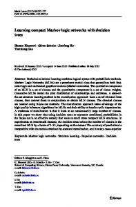
Table 1: Average F1 Algorithms MM-HM 1-best-MIRA-HM Subgradient-HM CDA1-PL-HM CDA1-ML-HM CDA2-PL-HM CDA2-ML-HM

and training time on CiteSeer dataset Average F1 Average training time 93.433 ± 1.41 90.282 min. 93.056 ± 3.18 11.772 min. 91.910 ± 2.37 12.655 min. 92.945 ± 2.94 11.824 min. 94.131 ± 2.25 12.738 min. 92.836 ± 2.55 11.869 min. 94.375 ± 2.13 12.887 min.

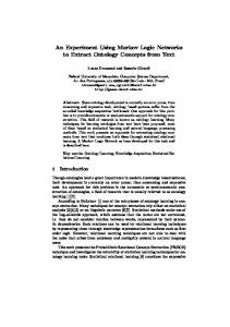
Table 2: MAP scores on Microsoft search query dataset Algorithms MLN1 MLN2 MLN3 CD 0.375 0.386 0.366 1-best-MIRA 0.366 0.375 0.379 Subgradient 0.374 0.397 0.396 CDA1-PL 0.380 0.395 0.396 CDA1-ML 0.379 0.389 0.385 CDA2-PL 0.382 0.397 0.398 CDA2-ML 0.380 0.397 0.397 training examples at once. In testing, we used exact MPE inference for Citeseer and used MCSAT to compute marginal probabilities for the web search query dataset since we want to rank the query results. The parameter σ of the Subgradient, CDA1 and CDA2 is set based on the performance on the validation set. All experiments used Hamming loss as the label loss function. For all online learning algorithms, we ran one pass over the training set and used the average weight vector to predict on the test set. For CiteSeer, we ran four-fold cross-validation (i.e. leave one topic out).

Metrics Like previous work, we used F1 , the harmonic mean of recall and precision, to measure the performance of each algorithm on Citeseer, and for the web query we used the MAP (Mean Average Precision) which measures how close the relevant results are to the top of the ranking.

Results and Discussion Table 1 presents the average F1 scores of different algorithms on Citeseer. On this dataset, CDA algorithms with maximal loss, CDA1-ML and CDA2-ML, have the best average F1 scores, and these results are better than those of 1best MIRA and the subgradient method (the differences with respect to the subgradient method are statistically significant). The F1 scores of CDA1-ML and CDA2-ML are also better than that of the batch max-margin algorithm (MM) since the batch learner can only uses approximate inference in training. Other advantages of online algorithms are in terms of training time and memory. On this dataset, the online learning algorithms took on average about 12-13 minutes for training while the batch one took an hour and a half on the same machine. Since online algorithms process one example at a time, they use much less memory than batch methods. Between CDA1 and CDA2, CDA2-ML is a little bit better but the difference is not significant. Regarding the comparison between maximal loss and predictionbased loss, the former is significantly better than latter on this dataset.

Table 2 shows the MAP scores of different algorithms on the Microsoft web search query dataset. The first row in the table is from Mihalkova and Mooney(2009) who used a variant of the structured perceptron (Collins 2002) called Contrastive Divergence (CD) (Hinton 2002) to do online weight learning for MLNs. It is clear that the CDA algorithms have better MAP scores than CD. For this dataset, we were unable to run offline weight learning since the large amount of training data exhausted memory during training. The 1-best MIRA has the worst MAP scores on this dataset. This behavior can be explained as follows. From the update rule of the 1-best MIRA algorithm, we can see that it aggressively updates the weight vector according to the loss incurred in each round. Since this dataset is noisy, this update rule leads to overfitting. This also explains why the subgradient algorithm has good performance on this data since its update rule does not depend on the loss incurred in each round. The MAP scores of CDA1 and CDA2 are not significantly better than that of the subgradient method, but their performance is more consistent across the three MLNs. CDA2 is better than CDA1 on this dataset since CDA2-ML is significantly better than CDA1-ML and CDA2-PL is comparable to CDA1PL. Regarding the loss function, in contrast to the results on Citeseer, the CDA algorithms with prediction-based loss are a little better than the ones with maximal loss especially for the case of CDA1, since aggressive update can lead to overfitting on noisy datasets. In summary, our new online learning algorithms CDA1 and CDA2 have generally better performance than existing max-margin online methods for structured prediction such as 1-best MIRA and the subgradient method which have been shown to achieve good performance in previous work. CDA2 is a little better than CDA1 especially on noisy datasets. Between the maximal loss and the predictionbased loss, the maximal loss is better than the predictionbased loss on clean datasets, but the latter is a bit better than the former on noisy datasets.

Crammer, K.; Dekel, O.; Keshet, J.; Shalev-Shwartz, S.; and Singer, Y. 2006. Online passive-aggressive algorithms. JMLR 7:551–585.

Conclusions and Future Work

Riedel, S. 2008. Improving the accuracy and efficiency of MAP inference for Markov logic. In UAI-08, 468–475.

We have presented a comprehensive study of online weight learning for MLNs. Based on the primal-dual framework, we derived new online algorithms for structured prediction and applied them to learn weights for MLNs and compared them to existing online methods. Our new algorithms generally achieved better accuracy than existing online methods on two large, real-world datasets. Since the new algorithms are not specific to MLNs, it would be interesting to apply them to other structured prediction models.

Acknowledgments This research is supported by a gift from Microsoft Research and by ARO MURI grant W911NF-08-1-0242. Most of the experiments were run on the Mastodon Cluster, provided by NSF Grant EIA-0303609.

References Boyd, S., and Vandenberghe, L. 2004. Convex Optimization. Cambridge University Press. Collins, M. 2002. Discriminative training methods for hidden Markov models: theory and experiments with perceptron algorithms. In EMNLP’02, 1–8.

Crammer, K.; McDonald, R.; and Pereira, F. 2005. Scalable large-margin online learning for structured classification. Technical report, Dep. of Computer and Information Science, Uni. of Pennsylvania. Getoor, L., and Taskar, B., eds. 2007. Statistical Relational Learning. Cambridge, MA: MIT Press. Hinton, G. E. 2002. Training products of experts by minimizing contrastive divergence. Neural Computation 14(8):1771–1800. Huynh, T. N., and Mooney, R. J. 2008. Discriminative structure and parameter learning for Markov logic networks. In ICML-08, 416–423. Huynh, T. N., and Mooney, R. J. 2009. Max-margin weight learning for Markov logic networks. In ECML PKDD 2009, Part I, 564–579. Kakade, S. M., and Shalev-Shwartz, S. 2009. Mind the duality gap: Logarithmic regret algorithms for online optimization. In NIPS-08, 1457–1464. Kautz, H.; Selman, B.; and Jiang, Y. 1997. A general stochastic approach to solving problems with hard and soft constraints. In Dingzhu Gu, J. D., and Pardalos, P., eds., The Satisfiability Problem: Theory and Applications, 573–586. AMS. Keshet, J.; Shalev-Shwartz, S.; Singer, Y.; and Chazan, D. 2007. A large margin algorithm for speech-to-phoneme and music-to-score alignment. IEEE Tran. on Audio, Speech & Language Processing 15(8):2373–2382. Lawrence, S.; Giles, C. L.; and Bollacker, K. D. 1999. Autonomous citation matching. In Proceedings of the third annual conference on Autonomous Agents. Lowd, D., and Domingos, P. 2007. Efficient weight learning for Markov logic networks. In PKDD-2007, 200–211. Mihalkova, L., and Mooney, R. J. 2009. Learning to disambiguate search queries from short sessions. In ECML PKDD 2009, Part II, 111–127. Poon, H., and Domingos, P. 2006. Sound and efficient inference with probabilistic and deterministic dependencies. In AAAI-2006. Poon, H., and Domingos, P. 2007. Joint inference in information extraction. In AAAI07, 913–918. Ratliff, N.; Bagnell, J. A.; and Zinkevich, M. 2007. (Online) subgradient methods for structured prediction. In AISTATS-07. Richardson, M., and Domingos, P. 2006. Markov logic networks. MLJ 62:107–136. Riedel, S., and Meza-Ruiz, I. 2008. Collective semantic role labelling with Markov logic. In CoNLL’08.

Shalev-Shwartz, S., and Singer, Y. Convex repeated games and Fenchel duality. In NISP-06. Shalev-Shwartz, S., and Singer, Y. 2007. A unified algorithmic approach for efficient online label ranking. In AISTATS-07. Shalev-Shwartz, S. 2007. Online Learning: Theory, Algorithms, and Applications. Ph.D. Dissertation, The Hebrew Uni. of Jerusalem. Singla, P., and Domingos, P. 2005. Discriminative training of Markov logic networks. In AAAI-05, 868–873. Singla, P., and Domingos, P. 2008. Lifted first-order belief propagation. In AAAI-08, 1094–1099. Taskar, B.; Chatalbashev, V.; Koller, D.; and Guestrin, C. 2005. Learning structured prediction models: a large margin approach. In ICML-05, 896–903. Taskar, B.; Guestrin, C.; and Koller, D. 2004. Max-margin Markov networks. In NISP-03. Tsochantaridis, I.; Hofmann, T.; Joachims, T.; and Altun, Y. 2004. Support vector machine learning for interdependent and structured output spaces. In ICML-04, 104– 112. Zinkevich, M. 2003. Online Convex Programming and Generalized Infinitesimal Gradient Ascent. In ICML-03, 928–936.