Markov random walk under constraint for discovering overlapping communities in complex networks Di Jin1, Bo Yang1, Carlos Baquero2, Dayou Liu1, Dongxiao He1 and Jie Liu1 1 College of Computer Science and Technology, Jilin University, Changchun 130012, China 2 CCTD/DI, University of Minho, Braga, Portugal E-mail:
[email protected],
[email protected],
[email protected],
[email protected],
[email protected] and
[email protected] Abstract. Detection of overlapping communities in complex networks has motivated recent research in the relevant fields. Aiming this problem, we propose a Markov dynamics based algorithm, called UEOC, which means, “unfold and extract overlapping communities”. In UEOC, when identifying each natural community that overlaps, a Markov random walk method combined with a constraint strategy, which is based on the corresponding annealed network (degree conserving random network), is performed to unfold the community. Then, a cutoff criterion with the aid of a local community function, called conductance, which can be thought of as the ratio between the number of edges inside the community and those leaving it, is presented to extract this emerged community from the entire network. The UEOC algorithm depends on only one parameter whose value can be easily set, and it requires no prior knowledge on the hidden community structures. The proposed UEOC has been evaluated both on synthetic benchmarks and on some real-world networks, and was compared with a set of competing algorithms. Experimental result has shown that UEOC is highly effective and efficient for discovering overlapping communities.
Keywords: analysis of algorithms, clustering techniques, network dynamics PACS: 89.75.Hc, 89.75.Fb, 02.10.Ox, 02.60.Cb 1. Introduction Many complex systems in real world exist in the form of networks, such as social networks,
biological networks, Web networks, etc., which are collectively referred to as complex networks. One of the main problems in the study of complex networks is the detection of community structure, i.e. the division of a network into groups of nodes having dense intra-connections, and sparse inter-connections [1]. In the last few years, many different approaches have been proposed to uncover community structure in networks; the interested reader can consult the excellent and comprehensive survey by Fortunato [2]. However, it is well known that many real-world networks consist of communities that overlap because nodes are members of more than one community [3]. Such observation is visible in the numerous communities each of us belongs to, including those related to our scientific activities or personal life (school, hobby, family, and so on). Another, biological example is that a large fraction of proteins simultaneously belong to several protein complexes [4]. Thus, hard clustering is inadequate for the investigation of real-world networks with such overlapping communities. Instead, one requires methods that allow nodes to be members of more than one community in the network. Recently, a number of approaches to the detection of overlapping communities in graphs have been proposed. One type, among these methods, is based on the idea of clique percolation theory, i.e. that a cluster can be interpreted as the union of small fully connected sub-graphs that share nodes [3, 5, 6]. Another type of method transforms the interaction graph into the corresponding line graph in which edges represent nodes and nodes represent edges, and then apply a known clustering algorithm on the line graph [7-10]. A third type of method, which our work belongs to, discovers each natural community that overlaps by using some local property based approach [11-13]. Though there are already some algorithms for detecting overlapping communities, which have been presented recently, there is still ground for improvements in the performance. Moreover, while the Markov dynamics model has been successfully used in the area for community detection [14-18], unfortunately, the existing approaches still largely lack the ability to deal with overlapping communities. To the best of our knowledge, only to recent works, available in pre-print format, constitute exceptions to this. Esquivel et al. [19] generalized the map equation method [16] by releasing the constraint that a node can only belong to one module codebook, and made it able to measure how well one can compress a description of flow in the network when we partition it into modules with possible overlaps. Kim et al. [20] extended the map equation method [16], which is originally developed for node communities, in order to find link communities in networks, and made it able to find overlapping communities of nodes by partitioning links instead of nodes. In this paper, an algorithm UEOC based on the Markov dynamics model is proposed to discover communities that share nodes. In the UEOC approach, so as to detect all the natural communities, a Markov random walk method is combined with a new constraint strategy, which is based on the corresponding annealed network [21], and used to unfold each community. Then, a cutoff criterion with the aid of conductance, which is a local community fitness function [22], is applied to extract the emerged community. These extracted communities will naturally overlap if this configuration is present in the network. Furthermore, a strong point in our approach is that UEOC is not sensitive to the choice of its only parameter, and needs no prior knowledge on the community structure, such as the number of communities.
2. Algorithm 2.1. Overview of the UEOC Let N = (V, E) denote an unweighted and undirected network, where V is the set of nodes (or vertices) and E is the set of edges (or links). We define a cover of network N as a set of overlapping communities with a high density of edges. In this case, some nodes may belong to more than one community. This is an extension of the traditional concept of community detection (in which each node belongs to a single community), to account for possible overlapping communities. In our case, detecting a cover amounts to discovering the natural community of each node in network N. The straightforward way to compute a cover of a targeted network is to repeatedly detect the community for each single node. This is, however, computationally expensive. The natural communities of many nodes often coincide, so most of the computer time is spent to rediscover the same modules over and over. For our algorithm, UEOC, a more efficient way is summarized as follows. S1. Pick node s with maximum degree, which has not been assigned to any community; S2. Unfold the natural community of node s by a Markov random walk method combined with a constraint strategy; S3. Extract the emerged community of node s by a cutoff criterion based on a conductance function; S4. If there are still nodes that have not been assigned to any community, repeat from S1. The core of UEOC is how to unfold and extract the natural community of each node, and this directly decides the performance of our algorithm. For the first goal, a Markov random walk method combined with a constraint strategy is proposed here, and this will result in making each community clearly visible. For the second one, a cutoff criterion based on the conductance function is presented, so as to precisely extract the emerged community. 2.2. Unfolding a community Given a network N = (V, E), consider a stochastic process defined on N, in which an imaginary agent freely walks from one node to another along the links between them. When the agent arrives at one node, it will randomly select one of its neighbors and move there. Assume that X = {Xt, t 0} denote the agent positions, and P{Xt = j, 1 j n} denote the probability that the agent arrives at node j after t steps walking. For t > 0 we have P{Xt | X0, X1, …, Xt-1} = P{Xt | Xt-1}. That is, the next state of the agent is completely decided by its previous state, which is called a Markov property. So, this stochastic process is a discrete Markov chain and its state space is V. Furthermore, Xt is homogeneous because P{Xt = j | Xt-1 = i} = pij, where pij is the transition probability from node i to node j. In terms of the adjacency matrix of N, A = (aij)nn, pij is defined as (1).
pij
aij
r air
(1)
Lets consider the Markov dynamics model above. Given a specific source node s for the agent, let sl (i ) denotes the probability that this agent starts from node s and eventually
arrives at an arbitrary destination node i within l steps. The value of sl (i ) can be estimated
iteratively by (2).
sl (i ) r 1 sl 1 (r ) pri n
(2)
Here, sl is called the l step transition probability distribution (vector). Note that the sum of the probability values arriving at all the nodes from source node s will be 1, i.e.
i 1 sl (i ) 1 . When step number l equals to 0, which means the agent is still on node s, then n
s0 ( s ) equals to 1 and s0 (i ) equals to 0 for each i s. As the link density within a community is, in general, much higher than that between communities, a random walk agent that starts from the source node s should have more paths, to choose from, to reach the nodes in its own community within l steps, when the value of l is suitable. On the contrary, the agent should have much lower probability to arrive at the nodes outside its associated community. In other words, it will be difficult for the agent to escape from its existing community by passing those “bottleneck” links and to arrive at other communities. Thus, in general, vector sl should broadly meet the condition (3) when the step number l is suitable. In this equation, Cs denotes the community where node s is situated. l l (3) : s (i ) s ( j ) iC s jC s
However, though the above Markov method is well suitable for some simple networks, such as the benchmark graphs in the Newman model [1] and some small real networks, it is not so effective for some complicated networks, like the benchmark graphs in the Lancichinetti model [23] (such as in the example of figure 1(a)) and some large-scale real networks. Furthermore, this method is very sensitive to the choice of the step number l, which depicts a crucial influence in its performance. There is an example, depicting vector sl and shown in figure 1(b). As we can see, the associated probability values of many within community nodes are smaller than that of the outside community nodes, thus it cannot unfold a clear community. This also means that sl does not fit condition (3) well enough for this relatively complicated network. Moreover, the result shown in this figure is the best performance case (when l equals to 3). It will become worse when step number l is greater or smaller than 3. In order to overcome these drawbacks, a Markov random walk method combined with a constraint strategy based on the corresponding annealed network is proposed here. The idea of our method arises in the intuition that a Markov random process on a network with community structure is different from that process on its corresponding annealed network without communities. Considering this, in each step, the probability that an agent starts from a specific source node s and arrives at each destination node i will be defined as the difference between its associated probability computed on the community network N and that on the corresponding annealed network R. Due to R having no community structure, the link density within a community in network N should be much higher than that in R, while the link density between communities in N should be much lower than that in R. Thus, under the constraint brought by the annealed network, this agent will be deterred from escaping it’s associated community and reach the nodes outside that community. This will also cause that,
the computed probability value of each within community node will be high, whilst that of each outside node will be relatively low and in most cases even equal to 0. Given network N = (V, E) with its degree distribution D, and the corresponding annealed network R (V' , E' ) with its degree distribution D' , it should be so that V V' , D D' while E E' . This means that N and R have the same degree distribution [21]. Let A = (aij)nn denote the adjacency matrix of network N. There will be D = diag(d1, … dn), in which d i j aij denotes the degree of node i. Assume that B = (bij)nn is the adjacency matrix (also called probability matrix) of R. We have bij d i d j / r 1 d r , which denotes the n
expected number of links (or called expected link probability) between nodes i and j. Let qij denote the transition probability from node i to node j on graph R. It will be defined as (4).
qij
bij
(4)
r bir
Considering the constraint generated by this annealed network R, let sl (i ) denote the probability that this agent starts from the source node s and eventually arrives at an arbitrary destination node i within l steps. The value of sl (i ) can be estimated iteratively by (5).
ls (i ) max sl (i ) It’s obvious that
n l 1 ( r ) r 1 s
n
(5)
ls (i )
r 1 ls (r ) n
r 1 sl 1 (r ) pri n
pri r 1 sl 1 ( r ) qri , 0
denotes the transition probability from node s to
node i within l steps on network N, while
r 1 sl 1 (r ) qri n
denotes that probability
computed on annealed network R. Furthermore, we make each sl (i ) always a nonnegative value. Since the sum of the probability values arriving at all the nodes from source node s should be 1, we also normalize sl (i ) after each step. An example for the proposed l step transition probability distribution sl is shown in figure 1(c). As we can see, the associated probability values of almost all within community nodes are greater than that of the outside community nodes, except for only a few special nodes whose community relations may be not very clear. In particular, there are 766 out of 903 outside community nodes whose probability values are 0. Thus, it’s obvious that, sl can meet condition (3) well, and unfold a very clear community for source node s. Moreover, this Markov process will convergence very well when step number l is greater than some value (in particular, 20 was found to be a good lower value). Thus, its performance is not as sensitive as before to the parameter l. Later, we will offer some detailed analysis on this parameter. Furthermore, most complex networks have power-law degree distribution, which means there are more paths arriving at the nodes with high degrees than those with low degrees. If not compensated, this will lead to detrimental effects when unfolding communities. Thus, we
take into account the effect of power-law degree distribution in complex networks, and propose a further improved l step transition probability distribution sl as defined as (6), where di denotes the degree of node i. Note that this equation is not iteratively computed.
ls (i )
sl (i ) di
, sl (i )
ls (i )
(6)
n ls (r ) r 1
There is an example for vector sl shown as figure 1(d). As we can see, this improved method can unfold a more clear community, and sl can meet (3) a little better than sl . 8 the transition probability distribution
the ID number of each node
0
200
400
600
800
1000
0
200 400 600 800 the ID number of each node
-3
the probabilities of within community nodes the probabilities of outside community nodes
7 6 5 4 3 2 1 0
1000
x 10
0
200
(a) 0.025 the probabilities of within community nodes the probabilities of outside community nodes
0.035 0.03 0.025 0.02 0.015 0.01 0.005
0
200
400 600 800 the ID number of each node
1000
the transition probability distribution
the transition probability distribution
1000
(b)
0.04
0
400 600 800 the ID number of each node
the probabilities of within community nodes the probabilities of outside community nodes 0.02
0.015
0.01
0.005
0
0
200
400 600 800 the ID number of each node
1000
(c) (d) Figure 1. An illustration for the Markov random walk method combined with our constraint strategy to unfold a community. (a) A benchmark network with power-law distribution of degree and community size by Lancichinetti model [23]. In this network, the number of nodes is 1000, the minimum community size is 20, the mixing parameter is 0.3, and the number of overlapping nodes is 400. Here we just consider the largest community, which contains 97 nodes. They are all put on the top of the nodes sequence. The selected source node s is the one with maximum degree in this community. (b) The generated l step transition probability vector according to (2). The best performance appears when l equals 3. (c) The generated l step transition probability vector according to (5). Its performance is insensitive to the increase of parameter l after it is greater than 20. (d) The generated l step transition probability vector according to (6). Its performance is insensitive to the increase of parameter l after it is greater than 20.
Based on this above idea, a method for unfolding the community, which contains a specific source node s, will be described bellow. This method is called UC (Unfolding Community). S1. Calculate the l step transition probability vector of node s, which is sl ; S2. Rank all the nodes according to their associated probability values in descending order, producing the sorted node list L. After these two steps, almost all the within community nodes will be ranked on the top of the sorted node sequence L. The target community has now clearly emerged and is ready for detection. Now, by properly setting a cutoff point (to be explained in the next section), we can precisely extract the community’s nodes. Proposition 1. The time complexity of the UC is O(ln2), where l is the step number of the random walk agent, and n corresponds to the number of nodes in network N. Proof. In S1, It’s obvious that the time to compute sl by (5) and (6) will be O(ln2). In S2, the time to rank sl will be O(nlogn), derived from quick sorting algorithms. Thus, the time complexity of the UC will be O(ln2). 2.3. Underlying mechanism in Unfolding Community Let an agent freely walk on a network N. For any node i, j and step number l, the probability
that the agent starts from node i and arrives at node j within l steps will be il ( j ) according to (2). This is a discrete Markov process. From the analysis of [24], according to large deviation theory, we know that the Markov chain has n local mixing states, and the i-th local mixing state corresponds to the number of communities i. In particular, if the network N has a well-defined community structure with k clear communities, this Markov chain will stay, in a stable way, in the k-th local mixing state during a period of time with a probability of 1, called a metastable state in this situation. According to this theory [24], all the local mixing times of the Markov chain can be estimated by using the spectrum of its Markov generator (normalized graph Laplacians) M = I−P, where I is the identity matrix and P is (pij)nn according to (1). For an undirected network, M is positive semi-definite and has n non-negative real-valued eigenvalues ( 0 1 2 n 2 ). Let Tient and Tiext be the entering time and exiting time of the i-th local mixing state. We have Tiext 1 (1 o(1)) . Reasonably, we can also use the exiting i
time of the (i+1)-th local mixing state to estimate the entering time of the i-th local mixing state. That is Tient Tiext 1 1/ i 1 . There is an example shown as figure 2. In order to depict this Markov process more clearly, we use a simple network and adopt the transition probability matrix instead of the transition probability vector here. Figure 2(a) shows a Newman network [1] which contains a known community structure with four clear communities. Figure 2(b) shows the spectrum of this network. Figure 2(c) shows the exiting time of each local mixing state. Especially, it also offers the entering time and exiting time of the 4-th local mixing state, which corresponds to a metastable state and evidences the real community structure of the network. Figure 2(d)-(f) depict the process of the Markov chain when it goes through the metastable state and finally
reaches the global mixing state. Figure 2(d) denotes the t1 ( t1 2 T4ent T5ext 1/ 5 ) step transition probability matrix when it begins to enter the metastable state which corresponds to the four clear communities. Figure 2(e) denotes the t2 ( t 2 7 T4ext 1/ 4 ) step transition probability matrix when it begins to exit this metastable state. Figure 2(f) shows the t3 ( t 3 20 T1ent T2ext 1/ 2 ) step transition probability matrix after it enters the global mixing state and eventually converges to this state, where we now have i 3 ( j ) d j / r d r t
1
1.6
0.9
1.4
0.8
1.2
20 0.7
40
10
8 X: 4 Y: 6.514
1
0.6 0.5 0.4
80
120 40
60
80
100
120
X: 5 Y: 0.6212
0.2
0.2
0.1
0
0
-0.2
0
20
40
60
0.06
40
0.05
60
0.04
80
0.03 0.02
100 0.01 120 100
120
the ID number of each node
the ID number of each node
the ID number of each node
20
80
100
120
0
140
0
20
40
60
0.025
40
0.02
60 0.015 80 0.01 100 0.005 120 40
60
80
100
120
140
(c)
20
20
80
i
(b) 0.07
60
80
i
(a)
40
X: 5 Y: 1.61
2 X: 4 Y: 0.1535
the ID number of each node
20
6
4
100
120
the ID number of each node
the ID number of each node
20
0.6 0.4
0.3 100
0.8
1/ i
60
i
the ID number of each node
for each node i and j. As we can see from this example, if a network has a community structure with k clear communities, there will be a short entering time (1/k+1) and a relatively long exiting time (1/k) for the k-th local mixing state, which denotes a metastable state. During this period of time, each community locally mixes together and we can observe the k communities of the network. Furthermore, the Markov chain will quickly converge to the global mixing state after it enters this state (> 1/2).
x 10 13
-3
12
20
11 40
10 9
60
8 80
7 6
100
5 120 4 20
40
60
80
100
120
the ID number of each node
(d) (e) (f) Figure 2. An example to demonstrate the characteristic of the iteration process for the Markov chain according to (2) on a benchmark network by Newman model [1]. (a) A Newman network consists of 128 nodes divided into four groups of 32 nodes. Each node has on average 14 edges connecting it to members of the same group and 2 edges to members of other groups, with the expected degree 16. (b) The spectral distribution (i) of this network. (c) The exiting time (1/i) of the local mixing state for each number of communities. (d) The t1 (t1 = 1/5) step transition probability matrix when the Markov chain begins to enter the metastable state. (e) The t2 (t2 = 1/4) step transition probability matrix when the Markov chain begins to exit the metastable state. (f) The t3 (t2 > 1/2) step transition probability matrix when the global stable state is finally reached.
0.1 40 0.08 60 0.06 80 0.04 100 0.02 120 20
40
60
80
100
120
the ID number of each node
0.045 20
0.04 0.035
40
0.03 60
0.025 0.02
80
0.015 100
0.01 0.005
120 20
40
60
80
100
120
the ID number of each node
the ID number of each node
0.12
20
the ID number of each node
the ID number of each node
Though the Markov chain of a random walk on the network contains a metastable state that corresponds to its real community structure, it will eventually reach the global mixing state, which denotes a trivial solution. For detecting communities, the followed intuition is that, if we can make the Markov chain remain and converge to this metastable state by deliberately adjusting transition probabilities, a nontrivial solution, which corresponds to the real community structure of the network, will be naturally attained due to this adjustment. Starting from this intuition, here we consider the difference between the Markov random process on a network N with community structure and that on its corresponding annealed network R without communities. It’s obvious that, the link density within a community in network N will be much higher than that in R, while the link density between communities in N will be much lower than that in R. Then, for any node i, j and step number l, if the l step transition probability from node i to node j computed on the community network N is no better (lower) than that computed on the annealed network R, we will have reason to believe that node i will have no chance of being in a same community of node j. Thus, we adjust and rescale the transition probability according to (5), which will make the probability that the constrained walker (agent) starts from node i and arrive at node j, within l steps, be null. It’s obvious that this will make the agent have almost no chance escaping from its own community, and the constrained Markov chain can hardly exit the metastable state that corresponds to the real community structure of the network. There is an example shown as figure 3, which corresponds to the case in figure 2. We find out that this constrained Markov chain can also enter the metastable state corresponding to the real community structure at time t1 = 1/5, which is shown as figure 3(a). However, it will not begin to exit the metastable state at time t2 = 1/4, but has almost converged to this state, which is shown as figure 3(b). At time t2 > 1/2, it has completely converged to the metastable state, which depicts the four clear communities shown as figure 3(c). As we can see from this example, the constrained Markov chain (according to (5)) has similar characteristics to the iteration process with the unconstrained Markov chain (according to (2)). However, the difference is that the unconstrained Markov chain will quickly converge to the global mixing sate after it enters this state (> 1/2), while the constrained Markov chain will quickly converge to the metastable sate that shows its k real communities after it enters this state (> 1/k+1). Therefore, we can make use of the spectrum of a network to approximate the convergence characteristics of the method UC. In fact, if the network has k real communities, the convergence time of the UC should be only a little longer than the entering time of the k-th local mixing state (> 1/k+1). 0.045 20
0.04 0.035
40
0.03 60
0.025 0.02
80
0.015 100
0.01 0.005
120 20
40
60
80
100
120
0
the ID number of each node
(a) (b) (c) Figure 3. An example that demonstrates the characteristics of the iteration process for the constrained Markov chain according to (5) on the network which is shown as figure 2(a). (a)
The t1 (t1 = 1/5) step transition probability matrix of the constrained Markov chain, which corresponds to figure 2(d). (b) The t2 (t2 = 1/4) step transition probability matrix of the constrained Markov chain, which corresponds to figure 2(e). (c) The t3 (t2 > 1/2) step transition probability matrix of the constrained Markov chain, which corresponds to figure 2(f). It is noteworthy that the above analysis on the characteristics of the iteration process of our UC method is in a close to ideal situation. It becomes more complex when dealing with networks depicting overlapping communities and some more complex topological properties, such as the sample network in figure 1(a) and for some large real-world networks. However, as we can see from figure 1, our UC method can still clearly unfold each node’s community and it’s also effective in this relatively complicated situation. Later, we will give some detailed analysis on the convergence characteristics of the UC in the experimental section of this article. 2.4. Extracting the emerged community As the community emerged from UC by computing the l step transition probability vector
sl , so that the associated probability values of the within community nodes are much greater than those of outside community nodes, the community associated to source node s can be easily distilled by designing a suitable cutoff criterion. At first we considered a simple method that takes the average probability value of all the nodes as a cutoff value, which is defined as i 1 sl (i ) / n . Then we extract the nodes n
whose associated probabilities are greater than as the detected community. For instance, in figure 4(b), the black line denotes the average probability as cutoff value. We find out that, although this can make all the within community nodes present in the same community, it will also include several outside nodes into this community. Let the structural similarity [25] of two arbitrary sets v and w be | v w | / | v | | w | . This average cutoff method will show that the structural similarity between the extracted community and the actual community is 0.8068. It’s obvious that the method is far from ideal to extract the emerged community on the sample network, even though this network already depicts some complexity. In order to improve this result and propose a more effective cutoff method, a well-known conductance function [22], corresponding to the weak definition of community [26], is used here in substitute of the less efficient boundary. The conductance can be simply thought of as the ratio between the number of edges inside the community and those leaving it. More formally, conductance (S) of a set of nodes S is (S) = cS/min(Vol(S), Vol(V \S)), where cS denotes the size of the edge boundary, cS = |{(u, v) : u S, v S}|, and Vol(S) = uS d u , where du is the degree of node u. Thus, in particular, more community-like sets of nodes have lower conductance. Moreover, this community function has some local characteristics, making it suitable to extract the emerged community.
Based on the ranked node list L obtained from UC, the emerged community can be easily distilled by computing the cut position that corresponds to the minimum conductance value, and taking it as the cutoff point along this ranked list of nodes. We can now summarize the method to extract the emerged community. This method is called EC (Extract Community). S1. Remove the nodes whose associated probability is 0 from the sorted node list L; S2. Compute the conductance value of the community corresponding to each cut position; S3. Take the community corresponding to the minimum conductance as the extracted one. Here we consider an example illustrating EC operation when extracting the emerged community, which is shown as figure 4 and corresponds to the case in figure 1. In figure 4(a), the blue curve denotes that the conductance value varies with the cut position. The pink triangle indicates the cutoff position corresponding to the minimum conductance value, while the black inverted triangle denotes the cutoff position corresponding to that of the average probability as cutoff value. In figure 4(b), the pink line denotes the cutoff value corresponding to the cut position that makes the conductance of the community to be minimal. It’s obvious that, EC can very effectively extract the community, which has emerged by UC, and the structural similarity between the extracted community and the real one is now much higher, 0.9379. 0.025 the sequence of conductance values the cut pos corresponding to the cut pos corresponding to min conductance
0.9
0.8
0.7
0.6
0.5
0
50 100 150 200 the cutoff position of the sorted nodes
250
the transition probability distribution
the corresponding conductance values
1
the probabilities of within community nodes the probabilities of outside community nodes average probability as cutoff value local min conductance as cutoff criterion
0.02
0.015
0.01
0.005
0
0
200
400 600 800 the ID number of each node
1000
(a) (b) Figure 4. An illustration EC extraction of the emerged community, which comes from figure 1. (a) The conductance value for the extracted community as a function of the cutoff position of the sorted node sequence L. These nodes are ranked according to their probabilities in descending order. There are only 234 of 1000 nodes whose associated probabilities are greater than 0, thus the x-axis is just in the range of 1~234. (b) Extracting the emerged community by cutting the l step transition probability vector sl via two types of cutoff criterions. Proposition 2. The time complexity of the EC is smaller than O(dn2), where d denotes the average degree of all the nodes. Proof. It’s obvious that S2 is the most computationally costly step in EC. We employ an incremental method to calculate the conductance value for each cut pos in the node list L. When the cut pos equals to 1, there is S1 = {L(1)} where L(1) denotes the first node in the
sorted node list L, cS1 = dL(1), Vol(S1) = dL(1), and Vol(V \S1) = m Vol(S1) where m is the number of edges in the network. When the cut pos equals to k, there should be Sk = Sk-1 {L(k)}, cSk = cSk-1 + dL(k) 2*|Sk NL(k)| where NL(k) denotes the neighbor set of node L(k), Vol(Sk) = Vol(Sk-1) + dL(k), and Vol(V \Sk) = m Vol(Sk). It’s obvious that, for each cut pos k, Sk NL(k) is the most costly step, whose time complexity is |Sk|*|NL(k)| = k*dL(k). Due to k being placed in the range of 1 k kmax where kmax