Jan 8, 2017 - given one input photo and some face sketch-photo pairs as the training dataset. .... three points: two eye centers and the mouth center. Each image is cropped .... ascending order. We call this fast version as Fast-RSLCR. We.
>
A SUBMISSION TO IEEE TRANSACTIONS ON NEURAL NETWORKS AND LEARNING SYSTEMS
A SUBMISSION TO IEEE TRANSACTIONS ON NEURAL NETWORKS AND LEARNING SYSTEMS
A SUBMISSION TO IEEE TRANSACTIONS ON NEURAL NETWORKS AND LEARNING SYSTEMS
A SUBMISSION TO IEEE TRANSACTIONS ON NEURAL NETWORKS AND LEARNING SYSTEMS
A SUBMISSION TO IEEE TRANSACTIONS ON NEURAL NETWORKS AND LEARNING SYSTEMS
62.5 62 61.5
63
62.5
62
61
61.5 62.2
60.5
RSLCR Fast-RSLCR
62
RSLCR Fast-RSLCR
RSLCR Fast-RSLCR
61
60 5
10
15
20
25
30
35
40
0
2
4
6
10
Overlap Size
(a)
(b)
Random Sampling Vs. SSIM Score
64
8
Patch Size
12
14
16
0
18
1
3
4
5
6
7
8
Search Length
(c)
6 Vs. SSIM Score
64
2
Number of nearest neighbors Vs. SSIM Score
63.4
63
63.2
63.5 63
60 59 58
63
SSIM Score (%)
61
SSIM Score (%)
SSIM Score (%)
62
62.5
62
57
62.8 62.6 62.4 62.2 62
61.5 RSLCR Fast-RSLCR
56
RSLCR Fast-RSLCR
55
61.8
61
0
200
400
600
800
1000
1200
1400
1600
61.6
0
0.1
0.2
0.3
0.4
Number of random sampled patch pairs
(d)
0.5
0.6
0.7
0.8
0.9
1
0
6
(e)
20
40
60
80
100
120
140
160
180
200
Number of nearest neighbors
(f)
Fig. 4. Statistics of SSIM scores under different parameter settings: (a) patch size, (b) overlap size, (c) search length, (d) number of random sampled patch pairs, (e) lambda, (f) number of nearest neighbors for Fast-RSLCR.
Regularization Parameterλ: It should be noted that when λ = 0 (refer to equation (5)), the locality constraint has no contribution to the reconstruction weight computation. Then equation (5) reduces to the LLE model in equation (1). The difference is that the entries of the data matrix X for the LLE method [4] is selected through K-NN while they are random sampled for RSLCR and Fast-RSLCR. From Fig. 4(e), on the one hand, it can be seen that when λ = 0, SSIM scores for RSLCR and Fast-RSLCR are 0.6250 and 0.6150 respectively compared with 0.5990 of the LLE method [4]. In addition, RSLCR and Fast-RSLCR run much faster than the LLE method (xx seconds for RSLCR, xx seconds for Fast-RSLCR, and xx seconds for LLE). This illustrates the effectiveness of the proposed random sampling strategy. On the other hand, when λ = 0.5, RSLCR and Fast-RSLCR achieve the best performance among all λ values, which is much larger than SSIM socres for λ = 0. This validates that the locality constraint does help to improve the performance. λ is set to 0.5 in this paper. Number of Nearest Neighbors for Fast-RSLCR: KNN is conducted in Fast-RSLCR to improve the computation efficiency. Fig. 4(f) presents the SSIM score against different number of nearest neighbors. Generally it grows with the increase of the number. To comprehensively comprise the time consuming and the SSIM socre, it is set to 200 in our experiments. From Fig. 4(d) it can be seen that directly random sampling 200 patches achieves an SSIM score of 0.6301 (at the time cost of 1.82s) while our proposed Fast-RSLCR (also use 200 sampled patches) could achieve an SSIM score of 0.6339
(at the time cost of 1.89s). It demonstrates the effectiveness of the proposed Fast-RSLCR method. B. Face Sketch Synthesis After the experimental setting for parameters, we set the patch size p = 20, overlap size o = 14, search length s = 5, the number for random sampling nrs = 800, the regularization parameter λ = 0.5, the number of nearest neighbors for FastRSLCR K = 200. For the CUHK student database, 88 pairs of face photo-sketch are taken for training and the rest for testing (the data has been partitioned in this database). For the AR database, we randomly choose 80 pairs for training and the rest 43 pairs for testing. For the XM2VTS database, we randomly choose 100 pairs for training and the rest 195 pairs for testing. Four state-of-the-art methods are compared: the LLE method [4], the SSD method [6], the MRF method [10], and the MWF method [11]. All synthesized sketches by the SSD method and the MWF method are generated from the source codes provided by the authors. For the MRF method, we use the codes from the implementation provided by authors of SSD [6]1 . Results of the LLE method is based on our implementations2 . The full list of synthesized sketches (both 1 The source codes for both the MRF method and the SSD method are available online: http://www.cs.cityu.edu.hk/∼yibisong/eccv14/index.html 2 Available online: http://www.ihitworld.com/RSLCR.html. On this project website, we will also release the source codes of both our proposed methods and the evaluation codes (objective image quality assessment codes and face recognition codes).
>
A SUBMISSION TO IEEE TRANSACTIONS ON NEURAL NETWORKS AND LEARNING SYSTEMS
A SUBMISSION TO IEEE TRANSACTIONS ON NEURAL NETWORKS AND LEARNING SYSTEMS
A SUBMISSION TO IEEE TRANSACTIONS ON NEURAL NETWORKS AND LEARNING SYSTEMS< SSIM Score on CUFS
100
LLE SSD MRF MWF Fast-RSLCR RSLCR
80
80 70
60 50 40
60 50 40
30
30
20
20
10
10
0.3
0.4
0.5
0.6
0.7
LLE SSD MRF MWF Fast-RSLCR RSLCR
90
Percentage (%)
Percentage (%)
70
0 0.2
SSIM Score on CUFSF
100
90
0 0.2
0.8
0.25
0.3
0.35
SSIM Score
0.4
0.45
0.5
0.55
0.6
SSIM Score
(a) Fig. 7.
9
(b)
Statistics of SSIM scores on (a) the CUFS database and (b) the CUFSF database. TABLE I AVERAGE TIME CONSUMPTION ( SECONDS ) TO GENERATE ONE SKETCH ON DIFFERENT DATABASES Methods
SSD
MRF
LLE
MWF
RSLCR
Fast-RSLCR
Programming language CUHK Student AR XM2VTS CUHK FERET
C++ 4.50 4.10 5.10 11.60
C++ 8.60 8.40 10.4 24.25
MATLAB 536.34 496.47 642.50 1591.95
C++ 16.10 15.33 18.80 45.20
MATLAB 18.79 19.10 18.14 17.66
MATLAB 1.82 1.73 2.36 1.44
TABLE II AVERAGE SSIM SCORE (%) ON THE CUFS DATABASE AND THE CUFSF DATABASE
CUFS (%) CUFSF (%)
SSD[6]
MRF[10]
LLE[4]
MWF[11]
Fast-RSLCR
RSLCR
54.20 44.09
51.32 37.34
52.58 41.76
53.93 42.99
55.42 44.56
55.72 44.96
TABLE III NLDA FACE RECOGNITION ACCURACY (%) BASED ON SYNTHESIZED SKETCHES FROM THE CUFS DATABASE AND THE CUFSF DATABASE Methods
LLE
SSD
MRF
MWF
Fast-RSLCR
RSLCR
CUFS (%) CUFSF (%)
91.12 (148) 61.76 (274)
90.24 (149) 70.92 (266)
87.29 (149) 46.03 (223)
92.13 (149) 74.15 (299)
98.35 (121) 73.41 (287)
98.38 (133) 75.94 (296)
synthesized sketches and corresponding ground-truth sketches drawn by the artist to train the classifier. The rest 188 sketches consists of the gallery. For the CUFSF database, we randomly choose 300 synthesized sketches and corresponding ground-truth sketches for training and the rest 644 synthesized sketches consist of the gallery. We repeat each face recognition experiment 20 times by randomly partition the data. Fig. 8 gives the face recognition accuracy against variations of the number of reduced dimensions by NLDA on the CUFS database and CUFSF database respectively. Table III presents the best face recognition accuracy at some dimension (the number in bracket). It can be seen that on the CUFS database, the proposed two methods outperform state-of-the-art methods a lot and on the more challenging CUFSF database, our
proposed RSLCR method also obtain the best performance with an accuracy of 75.94%. The Fast-RSLCR method has comparable performance with MWF. As shown in table II, although SSD achieves higher SSIM score than MWF, it has lower face recognition accuracy than MWF. This is because though SSD could clear face sketches (much less noise than MWF) it generates face deformations (e.g. mouth area as shown in Fig. 5 and Fig. 6). IV. C ONCLUSION In this paper, we presented a simple yet effective framework for face sketch synthesis based on random sampling and locality constraint. Random sampling in the offline stage could speed up the synthesis process since there is no need to
>
A SUBMISSION TO IEEE TRANSACTIONS ON NEURAL NETWORKS AND LEARNING SYSTEMS