The objective of the project is to design a text dependent speaker recognition system ...... shown below is run, the script file convert.txt is created (it contains all.
People’s Democratic Republic of Algeria Ministry of Higher Education and Scientific Research University M’Hamed BOUGARA – Boumerdes
Institute of Electrical and Electronic Engineering Department of Electronics Final Year Project Report Presented in Partial Fulfilment of the Requirements for the Degree of
MASTER In Electrical and Electronic Engineering Option: Telecommunications Title:
Text Dependent Speaker Recognition Using HTK Presented by: - BOUGUERRA Sara - SAHMI Nacera Supervisor: Dr. Abdelhakim DAHIMENE
Registration Number:……..../2016
Dedication
I dedicate this work to my beloved parents whom always help me and stand with me, I also dedicate it to my brothers Rayane and Lounes and my sister Rym, I don’t forget my best friends Imene and Nesrine . I want to give special appreciations and the best words to my husband Oussama, I dedicate this project to him and I thank him for his help and his precious advices. Thank you. BOUGUERRA Sara
I
Dedication
Dedication
I dedicate this work to my family. A special feeling of gratitude to my sisters Malha, Fezia, Nabila, Fatiha & Ferroudja for standing beside me and help me. I also dedicate it to my nephews and nieces. I dedicate again this work to my friends who encourage me and support me, and I give special thanks to my best friend Ahlam. Thank you. SAHMI Nacera
II
ACKNOWLEDGEMENT
ACKNOWLEDGEMENT
First and last, We thank ALLAH for all His blessing and strength that the gives us in completing this project We would like to sincerely thank our supervisor Dr A.DAHIMENE, for his guidance and support throughout this project, and especially for his confidence in us.
III
CONTENTS
TABLE OF CONTENTS
Dedication Acknowledgement Table of contents Abstract Introduction
…………………………………………………………………………… …………………………………………………………………............... …………………………………………………………………………… …………………………………………………………………………… ……………………………………………………………………………
I III IV VI 1
CHAPTER 01: SPEECH MECHANISEM 1.1 The process of speech production and perception in human beings …………………… 1.2 Generation of voiced and unvoiced sounds …………..…………………………………... 1.3 Speaker-specific characteristics of speech ……………………………………………….
04 06 07
CHAPTER 02: VOICE RECOGNITION USING MFCC's 2.1 Voice recognition principle 2.2 Mel-frequency Cepstrum 2.2.1 Steps in detail 2.2.2 Delta and energy
………………………………………………………………. ………………………………………………………………. ………………………………………………………………. ……………………………………………………………….
10 11 13 17
CHAPTER 03 : HIDDEN MARKOV MODELS 3.1 Markov chain ……………………………………………………………………………….. 3.2 Hidden Markov Model ‘HMM’ …………………………………………………………..… 3.2.1 HMM parameters ………………………………………………………….…. 3.2.2 HMM Network topology ……………………………………………………… 3.2.3 State-Time Trellis Diagram ……………………………………………………… 3.3 Hidden Markov Model Building Blocks ………………………………………………..... 3.3.1 Forward-Backward procedure ………………………………………….……… 3.3.2 Viterbi Algorithm ………………………………………………………….……… 3.3.3 Baum-Welch algorithm …………………………………………………………... 3.4 The relationship between HMMS Feature vectors and Speech ………………………...
20 21 21 22 23 23 24 25 26 27
CHAPTER 04 : IMPLEMENTATION IN HTK 4.1 Experiment ………………………………………………………………………………….. 4.2 Task Grammar ……………………………………………………………………………… 4.3 Creating Dictionary …………………………………………………………………………. 4.4 Preparation of the recorded data ………………………………………………………... 4.5 Coding the data ……………………………………………………………………………… 4.6 Creating monophone HMMs ……………………………………………………………...… 4.7 Fixing the silence models ………………………………………………………………... 4.8 Recognizer Evaluation …………………………………………………………………... 4.9 Discussion …………………………………………………………………………………….
IV
31 33 34 35 36 38 42 44 46
CONTENTS
Conclusion References
……………………………………………………………………………………….. ………………………………………………………………………………………..
59 60
APPENDIX A : AN OVERVIEW OF THE HIDDEN MARKOV MODEL TOOLKIT A.1 HTK software ……………………………………………………………………………… A.2 Available HTK Tools ……………………………………………………………………… A.2.1 Data preparation tools …………………………………………………………. A.2.2 Training tools ……………………………………………………………………….. A.2.3 Testing tools ……………………………………………………………………….. A.2.4 Analysis tools ……………………………………………………………………….. A.2.5 Standard HTK tool options …………………………………………………………. A.3 HTK files ……………………………………………………………………………………… A.3.1 Master Label File (MLF) …………………………………………………………... A.3.2 Configuration File …………………………………………………………………... A.3.3 Script files …………………………………………………………………………. A.3.4 HMM definition files ………………………………………………………………...
V
62 62 63 64 65 66 67 67 67 67 69 69
ABSTRACT
ABSTRACT
The objective of the project is to design a text dependent speaker recognition system using HTK, the HTK toolkit is used essentially for speech recognition, after understanding the theory of Hidden Markov Models, and the different processes HTK uses during recognition, the principle of Log likelihood probability, and the language Model are linked together to identify the speaker of an intended sentence chosen by the user and trained by the speaker wanted to be recognized. After several experiments, many threshold options were used, till arrived to the kinds of threshold playing a major role in speaker identification, a method for choosing thresholds has been formulated and it was applied for 10 speakers. The method for speaker identification worked successfully for all speakers, and the goal of recognizing a sentence that belongs to a particular speaker has been realized.
VI
INTRODUCTION
INTRODUCTION
The task of speech processing is being developed in the last years. Speech conveys different forms of information to the listener; one of them is the identification of a speaker. Speaker recognition is the process of automatically recognizing who is speaking on the basis of speaker features, which involves speaker identification and speaker verification. In speaker verification, the voiceprint is compared to the speaker voice model registered in the database wanted to be verified. The result of comparison is a measure of a similarity (score) from which rejection or acceptance of a verified speaker follows. At the identification stage, the voiceprint is compared with model voices of all speakers in the database. The comparison results are measures of the similarity from which the maximal quality is chosen. These systems can be further categorized as text dependant and text independent. By textindependence, it is meant that speaker can speak any utterance in a particular language, whereas in the case of text dependent systems the speaker is required to speak predefined pieces of text such as specific password. Several analytical approaches have been applied to the task of speaker recognition, many of which originate from speech recognition. Hidden Markov Models is the one of most common approaches and it is the one considered in this project. The HTK (Hidden Markov Model Toolkit) is a free and portable toolkit for building and manipulating hidden Markov models system (HMMs) ,developed at Cambridge university engineering department in 1989, and primary designed for speech recognition research. However speaker recognition has co-involved with this technology of speech recognition and speech synthesis because of the similar characteristics and challenges associated with each. This project seeks to look at the use of hidden Markov models to perform speaker recognition in the text dependent domain. This approach to speaker recognition will be analyzed through the design and implementation of HMMs using hidden Markov model toolkit. 1
INTRODUCTION
This project is divided into four chapter organized as follow: The first chapter describes briefly the process of speech production and perception in human beings. The second chapter deals with speech signal processing describing the various steps followed for feature vector extraction representing the acoustical characteristics of the speech signal using Mel-frequency cepstrum technique. The third chapter gives an overview on hidden Markov model theory The fourth chapter describes the structure of our speaker recognizer and the details of the implementation using HTK software, followed by the discussion of the results. Finally we end up with a conclusion along with some comments and suggestions.
2
CHAPTER 1 SPEECH MECHANISM 1.1 The process of speech production and perception in human beings 1.2 Generation of voiced and unvoiced sounds 1.3 Speaker-specific characteristics of speech
SPEECH MECHANISM
CHAPTER 1
Speech being the natural form of communication is the most basic and the most commonly used communication mean among human beings. For common people, it is just the sound waves coming out of the human month and perceived through ears. But there is a complex mechanism behind its production which will be dealt with in this chapter, as it is necessary for the development of our speaker recognition system. 1.1 The process of speech production and perception in human beings The process of speech production begins when the speaker formulates a message in his or her mind, to communicate with the listener via speech. The next step is the conversion of the message into a language code; this involves converting the message into a set of phonemes, comprising of correct sequence of words along with syntax, duration and loudness of sound.Once the language code is chosen, the speaker execute a series of neuromuscular commands cause the vocal cords to vibrate when appropriate and to shape the vocal tract such that the proper sequence of speech sounds is created, therefore producing an acoustic signal as the final output. The neuromuscular commands must simultaneously control all aspects of articulation1 including control of the lips, jaws, tongue, and velum. Once the speech waveform is generated and propagated to the listener, the speech perception process begins by analyzing the acoustical signal along the basilar membrane in the inner ear, thus spectrum analysis is performed on the incoming signal.Then a neural transduction process extract features such as duration of vocal cord vibration, intensity of the sound, resonant frequency of the vocal cord. And finally message comprehension is achieved.
1
The movement of organs like tongue, lips, jaws to produce speech sounds, and can be affected by many factors such as health of muscles used to produce the sound or neurological damage.
4
SPEECH MECHANISM
CHAPTER 1
SPEECH GENERATION TEXT
PHONEMS, PROSODY ARTICULATORY MOTIONS NeuroMuscular controls
Language code
Message Formulation
Discrete input
Vocal tract system
Continuous Input Acoustic Waveform
Waveform 50bPS
200bPS
2000bPS
30,000-50,000bPS Transmission Channel
Information Rate SPEECH RECOGNITION
SEMANTICS
PHONEMES, WORDS SENTENCES
FEATURE, EXTRACTION CODING
SPECTRUM ANALYSIS
Message understanding
Language Translation
Neural transduction
Basilar Membrane motion
DISCRETE OUTPUT
CONTINUOUS OUTPUT
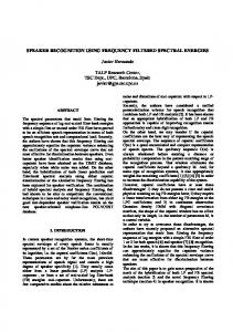
Fig 1.1 speech-production and speech perception process
Fig1.1 shows speech production and perception process and basic information rate of signal at various stages of the process. The discrete symbol information rate is the raw message and is rather low of 50bps (bits per second). After the language code conversion the information rate rises to about 200bps. In the neuromuscular control level the representation of the information in the signal becomes continuous with an equivalent rate of about 2000bps. At neuromuscular control where the movement of articulators and its coordination with brain comes in picture and transfer of information takes place about 30-50kbps at the acoustic signal level.
5
SPEECH MECHANISM
CHAPTER 1
For speech perception mechnism the information rate in the signal follows a inverse pattern of production process. Thus the continuous information rate at the basilar membrane is in the range of 30-50kbps. The higher level processing within
the brain converts the neural signals to a discrete
representation, which ultimately is decoded into a low-bit-rate message.[1] 1.2 Generation of voiced and unvoiced sounds Air enters the lungs via the normal breathing mechanism. As the air is expelled from the lungs through the trachea, it causes the tensed vocal cords within the larynx to vibrate producing so-called voiced speech sound, and it
Idea 1.2
results in speech waveform which is quasi-periodic in nature. The vocal cords are expressed as a simple vibration model, and the pitch of the speech changes according to adjustments in the tension of the vocal cords. When the vocal cords close, their vibration results in voiced sounds. when they are open, this vibration stops, and unvoiced sounds result.
Fig 1.2 A schematic diagram of the human vocal mechanism
6
SPEECH MECHANISM
CHAPTER 1
In the case of unvoiced sounds, the air flow pass through a narrow space formed by the tongue inside the month. A turbulent flow of air is produced and this is emitted as a noise-like sound, resulting in random speech waveform. [1] The classification of the speech signal into voiced and unvoiced provides a preliminary acoustic segmentation of speech, which is important for speech analysis. The analyses of speech signal is again very cumbersome due to its very fast changing parameters every 50 - 100 ms. For this speech analysis is performed in blocks or frames. These blocks are formed by windowing the speech signal for short duration for which the speech parameters are expected to be constant. Various methods are used for short time analysis of speech signal. In our project Mel Frequency analysis is used. [2] 1.3 Speaker-specific characteristics of speech The speaker-specific characteristics of speech are due to differences in physiological2 and behavioral aspects of the speech production system in humans.The main physiological2 aspect of the human speech production system is the vocal tract shape, larynx sizes and other parts of the production organs that are unique to each person. Moreover each speaker has his or her characteristic manner of speaking including the use of a particular accent, rhythm, intonation, style, choice of vocabulary and so
Idea 1.3 Speech conveys different forms of information to the listener. Along with the basic information about the language being spoken and the emotion, gender and the identity of the speaker also is a part of information.
on.These differences that might go unnoticed by the human ear will be captured by the system in the form of signal statistics and then exploited to distinguish one speaker from another one. Speaker recognition systems use a number of these features in parallel, attempting to cover these different aspects and employing them in a complementary way to achieve more accurate recognition. [3][4]
2
Physiology: understanding of the higher order mechanisms within the human central nervous system that account for speech production and perception in human beings.
7
SPEECH MECHANISM
CHAPTER 1
This chapter provides brief explanation of the speech production and perception mechanism in the human being, and illustrates how we can exploit the acoustic properties of the speech signal to identify the basic sound and the speakers, which help us in our recognition system.
8
CHAPTER 2 Voice Recognition Using MFCCs 2.1 Voice recognition principle 2.2 Mel-frequency Cepstrum
Voice Recognition Using MFCCs
CHAPTER 02
Automatic voice recognition technology is based on the digital processing
Idea 2.1
of the speech signal, the voice is the sound produced by the vocal organs of a vertebrate, especially a human, and it conveys infinite information, to represent the voice signal, two digital processes are used: Feature Extraction and Feature Matching. This chapter covers one of the mostly used feature extraction technique which is Mel Frequency Cepstrum Coefficients (MFCCs). First, the principles of voice recognition will be covered ,then the MFCC method is analyzed by explaining the various steps often used to obtain the coefficients. 2.1 Voice recognition principle To perform speech analysis, an input signal is taken from a microphone then the following operations are performed: Framing, windowing, Mel Cepstrum analysis and Matching (recognition) of the spoken word.
The training phase is the process of familiarizing the system with the voice characteristics of speakers registering, each speaker gives samples of its speech then the system builds a reference model for him after that comes the testing phase which is the actual recognition task, in this session an input voice is entered to the system then it is directly matched to the reference model stored before then a recognition decision is made.[5]
Voice recognition algorithmes
Training phase
Testing phase
Samples of the voice will be taken from each speaker, this builds a reference template
Ensuring that the input voice is matched with the reference template model then a recognition decision is made.
Fig 2.1 Voice recognition algorithms
10
Voice Recognition Using MFCCs
CHAPTER 02
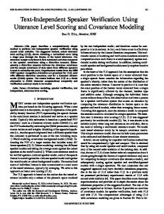
2.2 Mel-frequency Cepstrum Mel frequency Cepstrum is a representation of the short-termed power spectrum of a sound, MFCCs are the Mel Frequency Cepstrum Coefficients form the Cepstrum which is obtained by taking the inverse Fourier transform (IFT) of the logarithm of the spectrum of the signal. The following bloc diagram shows the different steps to obtain MFCCs.
Emphasis
Idea 2.2
Framing
Windowing The sounds that the human generates are filtered by the vocal tract (tongue, teeth,…) the role of the MFCCs is to represent the envelope that the vocal tract forms in the short time power spectrum of the voice signal.[5]
Voice input DFT
MFCCs Delta energy and
DCT
Mel filterbank
Fig 2.2 Block diagram showing the different steps. get MFCCs
The first step is Sampling of the signal at a given frequency
, and
emphasize higher frequencies, this is used to increase the energy of the signal at high frequencies. We suppose our signal is
] ]
]
]
(2.1)
11
Voice Recognition Using MFCCs
CHAPTER 02
The general steps to calculate the MFCCs can be summarized as follows: 1. Framing the signal into 20-50ms frame. 2. Finding the DFT then the periodogram estimate of the power spectrum. 3. Applying Mel filter-bank to power spectra, then for each filter an estimate of the energy is determined. 4. Taking Log of the filter-bank energies. 5. Computing the DCT of the resulting signal from step 4. The Mel scale is used to match the human perception to voice, the human ear differentiates small frequencies better than higher ones, this formula represents the relationship between the Mel scale and frequency
( )
(
)
(2.2)
6000
Idea 2.3 The first frame has samples, the second frame occurs after a frame skip duration that is , so the second frame begins after the first frame by samples, this means that they overlap by - samples.[6]
5000
M(f)
4000
3000
2000
1000
0
0
1
2
(1)
3
4
5 frequency
6
7
8
9
10 4
x 10
Fig 2.3 Graph of the Mel scale in terms of frequency
From the figure above it is noticed that as the frequency increases the slope of the graph increases, means that the distinction between adjacent frequencies becomes weak.
12
Voice Recognition Using MFCCs
CHAPTER 02
2.2.1 Steps in detail Framing: the signal is framed at a suitable value, generally from 20ms to 50ms, the frame length is measured in samples: (
)
Fig 2.4 shows the different parameters used in the encoding process applied to speech, framing is within this operation.
Window Duration SOURCERATE
WINDOWSIZE
Frame Period TARGETRATE ....etc
Parametervector size Bloc n
Bloc n+1 n+1
Speech Vectors
Fig 2.4 Speech encoding process [7]
Let’s call the time domain signal for the frame length is denoted as
], the framed signal or the signal
]
[n]
The Hamming window is applied to
[n] let’s call
[n] the resulting
signal.
13
Voice Recognition Using MFCCs
CHAPTER 02
]
]
]
]
(2.3)
(
)
(2.4)
Fig 2.5 Hamming window
] is computed.
DFT of the signal ]
∑
]
(2.5)
K is the length of the DFT. Now the Periodogram estimate of the power spectrum is calculated. ]
]
(2. 6)
Now we perform an M point FFT and keep only the first( coefficients. So that
(
)
)
14
Voice Recognition Using MFCCs
CHAPTER 02
To compute the Mel spaced filter-banks, an upper and lower frequency are chosen, then they are converted to Mel scale (equ 2.2), a number of filter banks is determined (let’s say 25), for an N number of filter banks N+2 points are needed, it is to find N frequency value between
and
(q is the frequency in Mels) the N Mel values are found using the following procedure:
(2.7) (
)
Then the result is N points linearly spaced between
and
, the
spacing between each point and the other is x. Now the resulting Mel scale values are converted to Hertz, and the are computed for a given frequency , the result is (
. )
]
(2.8)
Now filter-banks are created using the following function of
( )
(2.9) {
15
Voice Recognition Using MFCCs
CHAPTER 02
[fmin,fmax]=[0,8000]Hz Weight
1 0.5 0
0
1000
2000
3000
4000 Frequency (Hz)
5000
6000
Weight
1
8000
[fmin,fmax]=[300,3750]Hz
0.5 0
0
1000
2000
3000
4000 Frequency (Hz)
5000
6000
7000
8000
[fmin,fmax]=[4000,6000]Hz
1 Weight
7000
0.5 0
0
1000
2000
3000
4000 Frequency (Hz)
5000
6000
7000
8000
Fig 2.6 Mel Filter banks with different frequency ranges.
is the Mel frequency for
+2, the number of filter-banks that
can be used is [20-40]. To calculate filter-bank energies, each filter-bank
( ) is multiplied with
the periodogram estimate of the power spectrum, and then coefficients are added up, this results in N numbers giving us an idea of the energy in each filter-bank. ]
]
]
1. The Log for each filter-bank energy computed above is calculated. (
)
2. Finally the Discrete Cosine Transform is taken for each log energy computed above. The log energy for each filter-bank is
√ ∑
(
then
(
))
(2.10)
16
Voice Recognition Using MFCCs
CHAPTER 02
s so that that j= {1,2,…N}, are called Mel
Finally the coefficients
Frequency Cepstral Coefficients (MFCCs), the needed coefficients are the first 12 coefficients.[9] ] of the signal
To obtain the Cepstrum
], DFT of the Log of the
power spectrum is taken.[10] ]
∑
( ∑
]
)
(2.11)
Amplitude
0.5
Waveform 0
-0.5 -1
0
0.05
0.1
0.15
0.2
0.25
0.3
0.35
0.4
Magnitude (dB)
Time (s)
Idea 2.4 Stops are sounds where there is an occlusion of the vocal tract , in this case there is no nasal air flow so the air flow stops immediately, stops in English include voiceless sounds : p,t,k and voiced sounds like b,d,g. Sibilants are a kind of fricative sounds producing noisy airflow, the airflow in sibilants generates a groove in the tongue toward the teeth, this happens in the sounds s and z.[8]
50
Spectrum 0 -50 -100
0
500
1000
1500
2000
2500
3000
3500
4000
4500
5000
Frequency (Hz) Amplitude
800
Cepstrum
600 400 200 0
0
0.002
0.004
0.006
0.008
0.01
0.012
0.014
0.016
0.018
0.02
Quefrency (s)
Fig2.7 Audio waveform (letter a) with its Spectrum and Cepstrum
2.2.2Delta and energy The previous steps resulted in 12 cepstral coefficients for each frame, now the 13th feature is added, it is the energy of the signal within the frame, energy changes as the phone changes, for stops like the sounds p or k (see idea 2.4) the energy is low compared to its value when uttering sibilants like s or z. In the HTK toolkit the Energy is computed as the Log of the energy of the signal
]in N samples of a frame i.
17
Voice Recognition Using MFCCs
CHAPTER 02
∑
]
(2.12)
In reality, speech is not constant from frame to frame, in between, phones can exist and one may lose acoustic informations, this problem is solved by adding 12 delta coefficients (velocity features) and 12 acceleration (doubledelta) features. The delta feature for the cepstral value
at a sample of
time t is computed by the following regression formula. ∑
(
)
∑
(2.13)
is set by the user in configuration, if the above formula is applied to delta coefficients
( ) then acceleration coefficients are obtained (12 are
needed), the delta energy coefficient is obtained by replacing
(the cepstral
coefficient) by the energy of the frame, 2 more coefficients are needed the delta energy coefficient and the double delta energy coefficient. Now the following feature coefficients are calculated
12 mel frequency cepstral coefficients
12 delta cepstral coefficient
12 double delta cepstral coefficient
1 delta energy coefficient.
1 energy coefficient.
1 double delta energy coefficient.
Now each frame has 39 coefficients having the spectral features of the signal, these coefficient constitute what we call the feature vector.[10]
18
CHAPTER 3 HIDDEN MARKOV MODELS 3.1 Markov chain 3.2 Hidden Markov Model „HMM‟ 3.3 Hidden Markov Model Building Blocks 3.4 The relationship between HMMS Feature vectors and Speech
HIDDEN MARKOV MODELS
CHAPTER 03
This chapter provides the necessary information to understand the mechanism used for speaker recognition problem. To start, an introduction to the theory of hidden Markov model will be discussed as well as the basic algorithms used for the training and decoding process. In addition, state time trellis diagram will be discussed due to its use in finding the best path.
3.1 Markov chain A Markov chain is a process that consists of a finite number of states, with transitions among these states. A symbol is associated with each state and a probability is associated with each transition; such that the probability of being in a particular state depends only on the previous state.
Idea 3.1 In Markov model ,the probability of each symbol depends only on the preceding symbol not on the entire previous sequence.
Fig 3.1 A three-state chain
Fig 3.1 shows a three-state Markov chain, with transition probabilities a ij between states i and j. The symbols A, B and C are associated to states 1, 2 and 3 respectively. For example the transition from state 1 to state 2 generates symbol B as output. These symbols are called output symbols because Markov chain is thought of as a generative model; it outputs symbols as transition from one state to another. Now, given a sequence of output symbols generated by a Markov chain, we can retrace the corresponding sequence of states completely and unambiguously. An example of symbol sequence B A A C B B A C CC A is
20
HIDDEN MARKOV MODELS
CHAPTER 03
produced by transitioning into the following sequence of states: 2 1 1 3 2 2 1 3 3 3 1. Therefore in Markov chain the transitioning from one state to another is probabilistic, but the generation of the output symbols is deterministic. [11] 3.2 Hidden Markov Model „HMM‟ In the Markov model each state corresponds to one observable event
Idea 3.2
(output symbol). But this model is too restrictive to be applicable to many
HMM consists of two
problems of interest. Therefore Hidden Markov concept extends the model
stochastic processes. The
to include the case where the observation is a probabilistic function of the state.
Hence for each state a probability distribution is defined, that
first stochastic process is a Markov chain that is characterized by states and
specifies the probability for every observation symbol to be generated in
transition probabilities. The
that particular state. As each state can generate each observation symbol, it
second stochastic process
is no longer possible to see which state sequence generated an observation sequence as was the case for Markov models, the states are hidden, and hence the name of the model came.
produces emissions observable at each moment, depending on a statedependent probability distribution.
3.2.1 HMM parameters A Hidden Markov model can be defined by the following parameters:
Number of states in the model N.
Number of distinct observation symbols M.
Observation symbols
States will usually be indicated by
, , a state that the model is in at a
particular point in time will be indicated by q t . Thus qt = model is in state
at time t.
A probability distribution of transition between states A={aij}, where (
means that the
|
)
(3.1)
An observation symbol probability distribution b={bj(k)} in which (
|
)
(3.2) 21
HIDDEN MARKOV MODELS
CHAPTER 03
The initial state distribution
) where )
(3.3)
To indicate the complete parameter a set of a model the notation M= (A, B, ). [12] 3.2.2 HMM Network topology An HMM topology consists of the number of states with varied connections between states which depend on the occurrence of the observable symbol sequences being modeled
1
2 1
3
2
3
4
4
a
b
Fig 3.2: a) Ergodic model b) left to right model
The topology of Fig 3.2.a is called an ergodic network, since any state can be reached from any other state. This topology is inappropriate for speech recognition because speech consists of an ordered sequence of sounds. Generally left-to-right model is used Fig 3.2.b, where a state cannot be revisited once it is left, a transition can only stay in the same state or go to a higher numbered state. Consequently the transition matrix A is upper triangular. [13]
22
HIDDEN MARKOV MODELS
CHAPTER 03
3.2.3 State-Time Trellis Diagram A state–time trellis diagram shows the HMM states with all the different paths that can be taken through various states as time unfolds. Fig 3.3 illustrate a 4-state HMM and its state–time diagram. Since the number of states and the state parameters of an HMM are time-invariant, a state-time diagram is a repetitive and regular trellis structure. For a left–right HMM the state–time trellis has to diverge from the first state and converge into the last state. There are many different state sequences that start from the initial state and end in the final state. Each state sequence has a prior probability that can be obtained using Markov property.[14]
Fig 3.3: a) A 4-state left–right HMM, b) its state–time trellis diagram
3.3 Hidden Markov Model Building Blocks There are three basic HMM problems in finding the probability of speech feature vectors generated from an HMM. Firstly, evaluation, which finds the probability that a sequence of visible states was generated by the model M and this, is solved by the Forward-Backward algorithm. Secondly, decoding finds state sequence that maximizes probability of observation sequence using Viterbi algorithm. Lastly, training which adjusts model
23
HIDDEN MARKOV MODELS
CHAPTER 03
parameters to maximize probability of observed sequence. This last step is simply a problem of determining the reference speaker model for all speakers. The Baum-Welch re-estimation procedure is used for this case. 3.3.1 Forward-Backward procedure Idea 3.3
)and the
Consider the sequence of observation ) defined as:
forward variable
observation sequence,
)
)
(3.4)
i.e. The probability that the model has generated the partially observed sequence
Given HMM model and
at current state
. This variable
) can be solved
inductively by the forward procedure:
forward-backward algorithm finds the probability that the sequence comes with this model. In speaker identification
)
1. Initialize α at time t=1:
)
(3.5) For 1≤ i ≤N.
test, each speaker has a model, and identification is accomplished by finding the best fitting model as
2. Induction step:
)
[∑
]
)
)
(3.6)
determined by the highest probability.
For 1≤ t ≤ T-1; 1 ≤ ≤ N Once the variable α
)is the sum of this forward
) is calculated then
variable for the final observation over all the states. )
∑
Idea 3.4
)
(3.7)
This method is commonly known as the forward algorithm. Another way is to work backward from the ending state. The backward variable can be defined similar. )
)
i.e. probability of the sequence of observation after time t given state time t and the model M. again
(3.8)
Forward algorithm starts with the first observation and work forward through the data sequence until the end reached. This produces a probability which is the sum over all possible state sequence evaluated at
at
) can be solved inductively by the
backward procedure: 1. Initialize 𝞫 at time t=T:
)
(3.9)
24
HIDDEN MARKOV MODELS
CHAPTER 03
For 1≤ i ≤N )
2. Induction step:
∑
)
)
(3.10)
For t = T-1,T-2,….,1; 1≤ i ≤N ) is [15]:
Another efficient way of computing )
∑
[
)]
(3.11)
3.3.2 Viterbi Algorithm
Idea 3.5
Given the HMM M=(A, B, π) and the observation sequence ), veterbi algorithm finds the sequence of states ) that is most likely to have generated the given ) or
observations sequence.This boils down to maximize ).
equivalently Define variable
In speaker identification, Veterbi algorithm finds the path through a given speaker’s model that result in the highest probability. This algorithm is similar to the forward algorithm, with Σ replaced by max and additional backtracking.
) as the best path ( the path with the highest probability)
from the start into some state
at time t.
)
) (3.12)
By induction )
)
[
)
]
(3.13)
To recover the state sequence, this needs to keep tracks the argument which
Idea 3.6 In most cases, HMMs are implemented using log values to avoid underflow caused by the extremely small probabilities that occur when dealing with large models and large amount of the input data
maximizes the equation (3.13) for each t and j, and this is done via the array
).
The formal procedure for finding the best state sequence is as follows: 1. Initialisation at time t=1 )
) )
(3.14) (3.15) For 1≤ i ≤N 25
HIDDEN MARKOV MODELS
CHAPTER 03
2. Recursion: )
)
[ )
)
(3.16)
]
(3.17)
] )
[
For 2≤ t ≤ T; 1 ≤ ≤ N 3. Termination: [
)]
(3.18)
[
)]
(3.19)
4. Path ( state sequence ) backtracking: )
(3.20) For t=T-1, T-2,… 1.
3.3.3 Baum-Welch algorithm ) and general
Given finite training observation sequences
structure of HMM (numbers of hidden and visible states), determine HMM parameters M=(A, B, π) that best fit the training data and maximize the probability of the observation sequence given the model Define variable state
).
) as the probability of being in state at time t and in
at timet+1 given observation sequence . )
(
|
)
(3.21)
Idea 3.7 )
) In similar manner
)
)
)
)defined as the probability of being in state
(3.22) at time t
given the observation sequence . ) )
) ) ∑
) )
)
(3.23)
Application of these steps results in a new HMM ̅ by replacing M with ̅ , this procedure can be applied iteratively until there is minimal deference between M and ̅ in successive iteration.
(3.24)
26
HIDDEN MARKOV MODELS
CHAPTER 03
Expected number of transitions from state to state
=∑
)
(3.25)
)
(3.26)
Expected number of transitions out of state
=∑
Using the above formulas, a set re-estimation formulas for the parameter
,
A and B are: )
∑
)
∑
)
)
(3.27)
(3.28)
)
)
)
∑ ∑
)
(3.29)
[16]
3.4 The relationship between HMMS Feature vectors and Speech The observation sequence for speech recognition is a sequence of acoustic feature vectors (cepstral features). The acoustic feature vector represents information such as the amount of energy in different frequency bands. Each observation consists of 39 real valued features indicating spectral information. A reader to HMM theory would think that the hidden states of HMMs corresponds to phone units, and the words are sequences of these phones, but in fact if the frame duration is taken as 20ms, a simple phone like ‘ah’ or ‘s’ would take about 1second , this means it lasts 50 frames, this amount
27
HIDDEN MARKOV MODELS
CHAPTER 03
of frames cannot have an identical acoustic content, or feature vectors for each frame would not convey the same spectral information so the phone is modeled with more than 1 hmm state. The sequential nature of speech make strong constraints on transitions between states, the state is allowed to transition either to itself or to 1 succeeding
state,
the
standard
model
for
1
phone
is
shown
below
1 Start
2
Beginning
3
Middle
4
Final
5 End
Fig 3.4 standard 5-states HMM model for a phone.
The first and fifth states are non-emitting states, and the 3 others are emitting states.[10] To construct a sequence for a word having several phones, the start and end states of individual phones are mapped to the other phones.an example of state sequence for the word GOOD with succession of phones {GUH-D} is shown below
E E
S t t a r t
Fig 3.5.a composite word model for the word “GOOD”
28
HIDDEN MARKOV MODELS
CHAPTER 03
This chapter presented background materials on hidden Markov Modeling that will be used to implement a coherent speaker recognition system, in the next chapters feature vectors obtained from the previous chapter are used for speech recognition, and from the results of this, speaker identification can be performed using the acoustic model and the language model in parallel.
29
CHAPTER 4 Implementation in HTK 4.1 Experiment 4.2 Task Grammar 4.3 Creating Dictionary 4.4 Preparation of the recorded data 4.5 Coding the data 4.6 Creating monophone HMMs 4.7 Fixing the silence models 4.8 Recognizer Evaluation 4.9 Discussion
Implementation in HTK
CHAPTER 04
In this chapter, the implementation of a speaker recognition system using HTK will be presented. The main purpose is to construct a speech recognizer that can identify the speaker. The speaker of interest is the one uttering the training data. 4.1 Experiment In our experiment we have chosen the following English sentence: “enjoy your vacation”, having the following monophones in order:” eh n jh oy y ao r v ey k ey sh ah n” But for pronunciation purposes, silence models and short pauses must be included.
We have chosen 10 persons to pronounce the preceding sentence. The information about persons and the wav files corresponding to them are listed in the table below
Table I : the speakers with the audio files corresponding to them (the files highlighted are the ones used for training)
Speaker name
gender age audio file name
content
mi1.wav
Rym
F
11
mi2.wav
Enjoy your
mi3.wav
vacation
mi4.wav
1
mi5.wav mi6.wav sa1.wav
Sarah
F
23
2
sa2.wav
Enjoy your
sa3.wav
vacation
sa4.wav sa5.wav sa6.wav 8.wav
Nice day
na1.wav
3
Nacera
F
24
na2.wav
Enjoy your
na3.wav
vacation
31
Implementation in HTK
CHAPTER 04
na4.wav na5.wav na6.wav ra1.wav ra2.wav
Rayane
M
12
ra3.wav
Enjoy your
ra4.wav
vacation
ra5.wav 4
ra6.wav mon2r.wav
Monday
mon3r.wav va1.wav va2.wav Aziz
M
52
5
va3.wav
Enjoy your
va4.wav
vacation
va5.wav va6.wav va7.wav mondayvava.wav
Monday
monvava.wav sunvava.wav
Sunday
WAR1.wav WAR2.wav F
wardiya
44
WAR3.wav
Enjoy your
WAR4.wav
vacation
WAR5.wav
6
WAR6.wav MOTWARD.wav Beautiful mama1.wav mama3.wav
mama 7
F
45
mama4.wav
Enjoy your
mama5.wav
vacation
mama6.wav mama7.wav mama8.wav
32
Implementation in HTK
CHAPTER 04
mama9.wav wordmama.wav
Hello
word2mama.wav
My sister
word3mama.wav
My mother
ouss1.wav ouss2.wav
oussama
M
26
ouss3.wav
Enjoy your
ouss4.wav
vacation
ouss5.wav ouss6.wav 8
ouss7.wav oussword.wav
I am very intelligent
oussword2.wav
Amazing
ach1.wav ach2.wav
Achour
M
40
ach3.wav
Enjoy your
ach4.wav
vacation
ach5.wav ach6.wav
9
achword.wav
Je m‟appelle zazou
sami1.wav
Samira
F
35
sami2.wav
Enjoy your
sami3.wav
vacation
sami4.wav sami5.wav
10
sami6.wav samiword.wav
Thafath joue ballon
4.2 TaskGrammar
The following content is written in a text file we called “gram”
33
Implementation in HTK
CHAPTER 04
Fig 4.1 gram.txt A word network “wdnet” is created using Hparse
>Hparse gram.txt wdnet
4.3 Creating Dictionary
The dictionary is constructed manually, it contains the sentence defined in the grammar with the proper pronunciation , the script file is called dict.txt ,then the monophones occurring in it are placed in a new script file called monophones0.txt
Fig 4.2 dict.txt
Fig 4.3 monophones0.txt
34
Implementation in HTK
CHAPTER 04
4.4 Preparation of the recorded data
A word level script called words (speaker number).txt is constructed; it contains the transcriptions of what is said in each wav file used for training.
Fig 4.4 words1.txt
The following script “mkphones0.led.txt” is created
Idea 4.1 The meanings of EX,IS,DE EX is used to replace each word in words1.txt by the its pronunciation in the dictionary dict.txt. IS meansto insert a silence modelsilat the start and the end of each utterance.
Fig 4.5 mkphones0.led.txt
The phone level script called “phones (speaker number).txt” is
DE is used to delete short pause labels in the script phones01.txt in the incoming step
created by HLEd >HLEd –I „*‟ –d dict.txt –i phones01.txt mkphones0.led.txt words2.txt
The script file created is shown in Fig 4.4.
35
Implementation in HTK
CHAPTER 04
4.5 Coding the data
To code the data configuration files config.txt and config2.txt are created, the content of each of them is shown below. “config2.txt” content: # Coding parameters SOURCEKIND = WAVEFORM SOURCEFORMAT = WAV SOURCERATE = 226.5 TARGETKIND = MFCC_0_D_A TARGETRATE = 400000 SAVECOMPRESSED = T SAVEWITHCRC = T WINDOWSIZE = 1000000 USEHAMMING = T PREEMCOEF = 0.97 NUMCHANS = 26 CEPLIFTER = 22
Idea 4.2 The values of TARGETRARE and WINDOWSIZE are chosen in this way because they are suitable for the example of isolated word grammar, the default values given in htk book (p31) caused repititions of words in recognition.
NUMCEPS = 12 ENORMALISE = T “config.txt” content:
# Coding parameters TARGETKIND = MFCC_0_D_A TARGETRATE = 400000 SAVECOMPRESSED = T SAVEWITHCRC = T WINDOWSIZE = 1000000 USEHAMMING = T PREEMCOEF = 0.97 NUMCHANS = 26 CEPLIFTER = 22 NUMCEPS = 12 ENORMALISE = T 36
Implementation in HTK
CHAPTER 04
To extract the feature parameters Hcopy is used, before the command shown below is run, the script file convert.txt is created (it contains all the audio files listed in Table I), it is shown in Fig 4.7.
>HCopy -T 1 -C config.txt -S convert.txt Idea 4.3 To avoid errors in the command window when executing the command HERest, the test file in Fig 4.6 should be modified in the following way:
„*‟ will be * („ „ are deleted) Each line starts by “ and ends by . (Point)
Fig 4.6 phones01.txt
Fig 4.7 convert.txt
37
Implementation in HTK
CHAPTER 04
4.6 Creating monophone HMMs
The files train_sp(number of speaker).txt and proto.txt are created, proto.txt and train_sp1.txt are shown in Fig 4.8 and Fig 4.9 respectively.
Fig 4.8 proto.txt
38
Implementation in HTK
CHAPTER 04
After that, the command HCompV can be executed. >HCompV -C config.txt -f 0.01 -m -S train_sp1.txt -M hmm0_sp1 proto.txt
Idea 4.4 The data used for training are highlighted in Table I, in some htk examples 3 samples for training are enough, in this experiment we used 4 sentences for each speaker in order to make the results more accurate.
Fig 4.9 train_sp1.txt
This results in the creation of a new version of proto.txt and a script file vFloors.txt in the directory hmm0_sp1.
“proto.txt” (new version) content ~o 1 39 39 ~h "proto" 5 2 39 -6.817831e+000 -1.795901e+001 1.544357e+001 -1.344095e+001 …
39
Implementation in HTK
CHAPTER 04
We can see that the zero means and the unit variances in Fig 4.9havebeen replaced by the global speech means and variances. Now the 3 lines of proto.txt should be cut and pasted into the beginning of vFloors.txt, and the termMFCC_D_A_0 should be replaced by MFCC_0_A_D, then the resulting file is saved as macros.txt Now a new script file called hmmdefs.txt is created and the content of proto.txt (with the 3 lines cut) is copied for each monophone in monophones0.txt “macros.txt” content ~o 1 39 39~v varFloor1 39 3.823055e-001 8.135711e-001 4.871610e-001 5.969346e-001 6.232712e001
7.299178e-001
8.277286e-001
5.443348e-001
7.494858e-001
5.331665e-001 8.273274e-001 2.717662e-001 2.640264e+000 3.069856e002
6.211357e-002
4.464408e-002
4.441054e-002
5.292542e-002
4.015956e-002 8.592328e-002 5.867302e-002 5.088175e-002 6.099226e002
5.346099e-002
3.406173e-002
1.073499e-001
4.715789e-003
1.096903e-002 7.957620e-003 7.306530e-003 8.674498e-003 7.634106e003
1.744311e-002
1.153432e-002
8.500432e-003
1.175649e-002
8.656779e-003 6.373433e-003 8.520158e-003 “hmmdefs.txt” content ~h "ah" 5
40
Implementation in HTK
CHAPTER 04
2 39 -6.817831e+000 -1.795901e+001 1.544357e+001 -1.344095e+001 …. ~h "ao" 5 …
To re-estimate the HMM parameters Baum-welch training is used by the command HERest, the models are re-estimated 3 times , each time putting the re-estimated fileshmmdefs.txt and macros.txt in a new directory, in this case hmm1_sp1, hmm2_sp1 and hmm3_sp1, macros.txt is put also in these files but the values in it doesn‟t change. The following command is typed
>HERest -C config.txt -I phones01.txt -t 250.0 150.0 1000.0
-S train_sp1.txt –
H hmm0_sp1/macros.txt -H hmm0_sp1/hmmdefs.txt -M hmm1_sp1 monophones0.txt >HERest -C config.txt -I phones01.txt -t 250.0 150.0 1000.0
-S train_sp1.txt
–H hmm1_sp1/macros.txt -H hmm1_sp1/hmmdefs.txt -M hmm2_sp1 monophones0.txt >HERest -C config.txt -I phones01.txt - t 250.0 150.0 1000.0
-S train_sp1.txt
–H hmm2_sp1/macros.txt -H hmm2_sp1/hmmdefs.txt -M hmm3_sp1 monophones0.txt
41
Implementation in HTK
CHAPTER 04
We see that the values of means and variances change each time and the values in the transition matrix too. 4.7 Fixing the silence models
Now the silence models should be fixed.
Short pause (sp) is a one emitting state model, so that state 3 of sil is state 2 of sp, so sp model is created by opening a new directory hmm4, then copying the two files hmmdefs.txt and macro.txt from hmm3 then the hmm of sil is copied then pasted, after that the name is changed to sp and state 3 of sil becomes state2of sp, the remaining parameters are modified to obtain a 1 emitting state sp model. A part of hmm4_sp1/hmmdefs.txt is shown below in fig 4.10
Fig 4.10 a part of hmm4_sp1/hmmdefs.txt
We create a new text file called sil.hed.txt
Fig 4.11 sil.hed.txt
The AT command adds transitions to the transition matrices and TI creates a tied state called silst.
42
Implementation in HTK
CHAPTER 04
The following command is executed. >HHEd
-H
hmm4_sp1/macros.txt
-H
hmm4_sp1/hmmdefs.txt
-M
hmm5_sp1 sil.hed.txt monophones1.txt
We notice in hmm5_sp1 that the values in sil.hed.txt are added to the transition matrices of sil and sp.
The re-estimation is applied again to generate hmmdefs.txt and macro.txt in 2 other directories hmm6_sp1 and hmm7_sp1, in this case sp is added to the phones in monophones0.txt then it is saved as monophones1.txt, the following commands are run.
>HERest -C config.txt -I phones01.txt - t 250.0 150.0 1000.0
-S train_sp1.txt
–H hmm5_sp1/macros.txt -H hmm5_sp1/hmmdefs.txt -M hmm6_sp1 monophones1.txt >HERest -C config.txt -I phones01.txt - t 250.0 150.0 1000.0 –H
hmm6_sp1/macros.txt
-H
hmm6_sp1/hmmdefs.txt
-S train_sp1.txt -M
hmm7_sp1
monophones1.txt
Before getting into the recognition command, audio files from several speakers are entered to test the recognition process. The files are in test.txt, the content of each of them is mentioned in Table I , the files occurring in test.txt are all files in Table I ,except the ones used for training(highlighted in table I) this is for all speakers except for speaker 7 (MAMA), for this speaker we tested the files already trained to see the difference. The content of test.txt data\sa5.mfc data\sa6.mfc data\na5.mfc data\na6.mfc…
43
Implementation in HTK
CHAPTER 04
4.8 Recognizer Evaluation HVite is run for the speaker 1 model and the final recognition results are stored in result.txt >HVite -T 1 -H hmm7_sp1/macros.txt -H hmm7_sp1/hmmdefs.txt -S test.txt -i results.txt -w wdnet -p 0.0 -s 5.0 dict.txt monophones1.txt The following results appear on the command window:
(a)
44
Implementation in HTK
CHAPTER 04
(b)
(c)
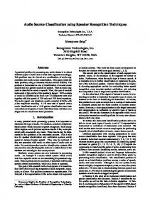
Fig 4.12 (a)-(b)-(c) Recognition results for speaker 1
45
Implementation in HTK
CHAPTER 04
The information listed for each utterance are: Idea 4.5
The recognized string: in fact whatever the speaker say, HTK toolkit recognizes only what is in its grammar, since we have written one single sentence in grammar, it recognizes nothing but “Enjoy your vacation”. The total number of frames in the utterance: this gives an idea of the length of the sentence. The average log probability per frame: is the total acoustic likelihood divided over the number of frames (see idea 4.5). The total acoustic likelihood: the total log probability. The total language model likelihood: since the recognizer test the sentence as a whole there is no word –end transitions so the language model likelihood is set to 0.
For an acoustic model of T frames, every frame from the start node to the exit node passes through T emitting HMM states, the log probability is computed by summing the individual transitions in the path and the probability of each emitting state generating the particular observation, the decoder finds the path through the network having the highest log probability. [7]
The average number of active models 4.9 Discussion The speaker of the trained sentence „Enjoy your vacation‟ can be identified by ordering the average log probability per frame in ascending order, the utterance with the higher average Log probability per frame (the closest to zero), corresponds to the speaker in interest, for speaker1, from Table I the utterances corresponding to the speaker “ RYM” are mima5.wav and mima6.wav, from Fig 4.12 , the audio file having the highest average log probability is mi6.mfc with a value -61.1875 then comes mi5.mfc with -61.5138, both correspond to the speaker Rym. In order to identify the speaker only, without caring for other people, thresholding can be applied, in this case the parameters used for thresholds are the beam searching using –t and word end pruning using –v choosing a value of 200 for the beam searching and 200 for the word end pruning means that any model or any observation whose log probability token falls more than 200 below the maximum for all models is deactivated
46
Implementation in HTK
CHAPTER 04
or killed ,furthermore, tokens from word end nodes that falls more than 200 below the maximum word end likelihood are killed. The following command is executed. >HVite -T 1 -H hmm7_sp1/macros.txt -H hmm7_sp1/hmmdefs.txt -S test.txt -i results1.txt -w wdnet -p 0.0 –t 200 –v 200 -s 5.0 dict.txt monophones1.txt The results in the command window are shown in Fig 4.13, using thresholding caused 4 audio files to be recognized, fromTable I , it is remarked that the files mi5.mfc and mi6.mfc belongs to the speaker which means it is a good result, but two other files ra4.mfc and ra5.mfc belong to speaker4 that is Rayane , in fact the values of average likelihood per frame for the two speakers are close, to detect only the audio file corresponding to the speaker the threshold in –t option can be decreased, let‟s use –t 100. >HVite -T 1 -H hmm7_sp1/macros.txt -H hmm7_sp1/hmmdefs.txt -S test.txt -i results1.txt -w wdnet -p 0.0 –t 100 –v 200 -s 5.0 dict.txt monophones1.txt
47
Implementation in HTK
CHAPTER 04
(a)
(b)
Fig 4.13 (a)-(b) Recognition results for speaker 1 using thresholding
48
Implementation in HTK
CHAPTER 04
(a)
(b)
Fig 4.13 (a)-(b) Recognition results for speaker 1 using thresholding 2
49
Implementation in HTK
CHAPTER 04
Let‟s apply the same procedure to speaker2 (Sarah), the results are shown in Fig 4.14.
(a)
(b)
Fig 4.14 (a)-(b) Recognition results for speaker 2 using thresholding
50
Implementation in HTK
CHAPTER 04
In speaker2 , 2 audio files sa5.mfc and sa6.mfc are detected, both correspond to speaker2, but one may not know whether they both belong to the speaker in interest, that is why the threshold must be decreased again to obtain only 1 audio file detected.
(a)
(b)
Fig 4.14 (a)-(b) Recognition results for speaker 2 using thresholding 2
51
Implementation in HTK
CHAPTER 04
Then the process of Thresholding can be summarized in the following chart Chart I: Method to use Beam searching in recognizing MFC files
Start
F0 = 200 i=0 i=0 is executed -t Fi –v200 i=i+1 No yes
0 mfc files detected previously too?
Yes
More than 1 mfc file is detected?
No
yes
0 mfc files detected?
The speaker exists in the list of mfc files? Yes
No End
No
52
Implementation in HTK
CHAPTER 04
The results for speaker 3 is shown in Fig 4.15 below
(a)
(b)
Fig 4.15 (a)-(b) Recognition results for speaker 3 using thresholding
53
Implementation in HTK
CHAPTER 04
Table II: Recognition results in the command window using Tresholding: several iterations are perfomed according to Chart I till recognition is perfomed successfully (green color), “S “means the sentence “ENJOY YOUR VACATION”
Speaker number
Speaker name
F value in –t option
MFC files detected
Rym
200
Sarah
100 200
mi5.mfc mi6.mfc mi6.mfc sa5.mfc sa6.mfc sa5.mfc sa6.mfc sa6.mfc na6.mfc ra4.mfc ra5.mfc 0 ra4.mfc va5.mfc va6.mfc va5.mfc va6.mfc va6.mfc WARD5.mfc WARD6.mfc WARD5.mfc WARD6.mfc WARD5.mfc mama5.mfc mama6.mfc mama7.mfc mama8.mfc ra5.mfc ra4.mfc mama5.mfc mama6.mfc mama7.mfc mama8.mfc mama6.mfc mama7.mfc mama8.mfc mama6.mfc mama7.mfc mama8.mfc mama6.mfc
1
100 2 3
Nacera Rayane
50 200 200
Aziz
100 150 200
4
5
100
Wardiya
50 200 100
6 Mama
50 200
100
7
50
25
12.5
Average Log Content probability of per frame MFC file -65.5138 S -61.1875 S -61.1875 S -56.7441 S -49.9066 S -56.7441 S -49.9066 S -49.9066 S -65.9774 S -45.4212 S -59.8998 S 0 0 -45.4212 S -68.7027 S -68.0087 S -68.7027 S -68.0087 S -68.0087 S -57.8368 S -59.6924 S -57.8368 S -59.6924 S -57.8368 S -64.9699 S -50.0685 S -46.8897 S -46.5117 S -100.6124 S -92.3274 S -64.9699 S -50.0685 S -46.8897 S -46.5117 S -50.0685 S -46.8897 S -46.5117 S -50.0685 S -46.8897 S -46.5117 S -50.0685 S
Recognition rate?
50% 100% 50% 50% 100% 100% 50% 0% 100% 50% 50% 100% 50% 50% 100%
16.66%
25%
33.33%
33.33% 33.33%
54
Implementation in HTK
6.25
3.125
1.5625 2.34375 1.953125 2.1484375 0
Oussama
8
CHAPTER 04
mama7.mfc mama8.mfc mama6.mfc mama7.mfc mama8.mfc mama6.mfc mama7.mfc mama8.mfc 0 mama6.mfc mama8.mfc 0 mama6.mfc
-46.8897 -46.5117 -50.0685 -46.8897 -46.5117 -50.0685 -46.8897 -46.5117 0 -50.0685 -46.5117 0 -50.0685
S S S S S S S S 0 S S 0 S
mama8.mfc 0 0
-46.5117 0 0
S 0 0
33.33%
33.33%
0% 50% 0% 50% 0% 0%
1.8798828 0 0 0 0% 13 2.0141598 mama6.mfc -50.0685 S 50% 15 mama8.mfc -46.5117 S mama6.wav and mama8.wav belong to the same speaker Mama and they are too close in average log probability, and also they are detected together for very small values of thresholds, this is because they are the trained data for speaker 8, as mentioned before. 200 ra5.mfc -91.0644 S ra4.mfc -89.9052 S 16.66% va6.mfc -85.8467 S ouss5.mfc -63.1234 S ouss6.mfc -60.6256 S ouss7.mfc -58.9640 S ouss5.mfc -63.1234 S 33.33% 100 ouss6.mfc -60.6256 S ouss7.mfc -58.9640 S 50 ouss5.mfc -63.1234 S 33.33% ouss6.mfc -60.6256 S ouss7.mfc -58.9640 S 25 ouss5.mfc -63.1234 S 33.33% ouss6.mfc -60.6256 S ouss7.mfc -58.9640 S 12.5 ouss5.mfc -63.1234 S 33.33% ouss6.mfc -60.6256 S ouss7.mfc -58.9640 S 6.25 ouss5.mfc -63.1234 S 50% ouss6.mfc -60.6256 S 3.125 ouss6.mfc -60.6256 S 100%
55
Implementation in HTK
9
Achour Samira
10
200 200
100 50
CHAPTER 04
ach5.mfc WAR5.mfc Sami5.mfc sami6.mfc sami5.mfc sami6.mfc sami5.mfc
-81.1658 -133.8591 -60.6665 -57.5264 -60.6665 -57.5264 -62.9390
S S S S S S S
100% 33.33%
50% 100%
From the above table it is remaked that recognition was perfomed successfully for all the 10 speakers . As seen in theory, each HMM is composed of a sequence of phone models, each phone model contains subphone states. To solve the problem of decoding , in the speech recognition task, the best sequence of words is the one that maximizes the two factors,the maximum lnguage model prior
and the acoustic likelihood
.[10]
(4.1)
This fact was used for Speaker identification, the thresholding of the language model likelihood enables the detection of the intended sentence “ENJOY YOUR VACATION”, and the maximum Log probability thresholding allows the speaker identifcation, because the more the testing voice is closer to the voice used for training, the Maximum log probability and the average Log acoustic likelihood become higher, the use of the value 200 as an initial value in the -t option was set arbitrarily, because it suits all speakers, in the –v option (the word end puning), the value 200, was set by default as the optimum case because withsmaller values, the model risks of not detecting any mfc file (see Fig 4.16)
56
Implementation in HTK
CHAPTER 04
(a)
(b)
Fig 4.16 (a)-(b) Recognition results when setting the word end pruning threshold to 100
57
Implementation in HTK
CHAPTER 04
Finally, the following facts can be deduced from this model.
This model is a text dependent , because when using thresholds the sentences said by speakers that are other than “ENJOY YOUR VACATION”, like MOTWOARD.mfc, wordmama.mfc and oussword.mfc (see TABLE I), are deactivated even when using initial values of thresholds.
This method is a fast method , for most of speakers a small number of iterations (even when more than 1 file corresponding to the text and to the speaker exists), is enough to recognize one sentence allowing the user to say: it belongs to the speech (“ENJOY YOUR VACATION”) and it is uttered by the speaker in interest.
This model can be generalized for a high number of speakers, because it is trained with 10 speakers from different ages and genders.
58
CONCLUSION
CONCLUSION
The concept of constructing text dependent speaker recognition has been presented in this project. Since the speaker recognition is a new idea in the field of signal processing, and speech recognition was developed earlier, the mathematical models that construct the speech recognizer were used to identify a speaker uttering some training data. To achieve the results, a lot of experiments have been done respecting the HTK toolkit procedure. Furthermore, the results were presented in HTK command window instead of a text file. By using the concept of thresholding, only the intended audio file corresponding to the speaker in interest appears, and the audio files of other speakers in addition to the sentences other than the trained one, are deactivated even if they belong to the speaker in interest. As a further, some recommendations are suggested for researchers in the filed: The recognizer live in HTK needs to be developed to function in a faster rate. Constructing a big grammar containing all sentences in English, in order to recognize anything the speaker can say. The development of HTK as software having an appropriate user interface to avoid dealing with the traditional command window.
95
REFERENCES
REFERENCES [1] Rana, D. S. (2012). The process of speech recognition, perception, speech signals and speech production in human beings.International Journal of Advanced Research in Computer Engineering & Technology (IJARCET), 1(9), pp-156. [2] Harish ChanderMahendru,(January 2014)."Quick Review of Human Speech Production Mechanism ",Department of Electronics & Communication Engg., Haryana Engineering College,International Journal of Engineering Research and Development, Volume 9, Issue 10 . [3] http://www.barcode.ro/tutorials/biometrics/voice.html (03/2016) [4] CHOUGUI &HACIANE(2015). "speaker recognition system using htk",Master final report, Institute of Electrical and Electronics Engineering,.University of Boumerdes. [5] Tiwari, V. (2010). MFCC and its applications in speaker recognition.International Journal on Emerging Technologies, 1(1), 19-22. [6] Rajsekhar, A. (2008). Real time Speaker Recognition using MFCC and VQ. M. TechThesis, National Institute of Technology, Rourkela, India. [7] Steve, Y., Gunnar, E., & MARK, A. (2009). The HTK book (for HTK Version 3.4).Steve Young, Gunnar Evermann, Dan Kershaw, Gareth Moore, Julian Odell, Dave Ollason, ValtchoValtchev, Phil Woodland. [8] https://en.wikipedia.org/wiki/Manner_of_articulation (05/2016) [9] http://practicalcryptography.com/miscellaneous/machine-learning/guide-mel-frequencycepstral-coefficients-mfccs/ (03/2016) [10] Martin, J. H., &Jurafsky, D. (2000). Speech and language processing.International Edition. [11] Makhoul, J., & Schwartz, R. (1995). State of the art in continuous speech recognition. Proceedings of the National Academy of Sciences, 92(22), 9956-9963. [12] AI, R. T., Spraakherkenning, A., Wiggers, I. P., &Rothkrantz, L. J. M. (2003). AUTOMATIC SPEECH RECOGNITION USING HIDDEN MARKOV MODELS. [13] Kotwal, P., & Dixit, M. R. Learning Assistant in Educational Field Using Automatic Speech Recognition. [14] Vaseghi, S. V. (2008). Advanced digital signal processing and noise reduction. John Wiley & Sons. [15] Jackson, P. (2011). HMM tutorial. Centre for Vision Speech Signal Processing, University of Surrey. Web. [16] Rabiner, L. R. (1989). A tutorial on hidden Markov models and selected applications in speech recognition. Proceedings of the IEEE, 77(2), 257-286.
60
APPENDIX A AN OVERVIEW OF THE HIDDEN MARKOV MODEL TOOLKIT A.1 HTK software A.2 Available HTK Tools A.3 HTK files
AN OVERVIEW OF THE HIDDEN MAROV MODEL TOOLKIT
The subject of this appendix is Hidden Markov Toolkit HTK, a collection of software libraries and tools for manipulating Hidden Markov models are presented. The architecture of the toolkit will be described and an overview of the tools used in our speaker recognizer will be given. A.1 HTK software The Hidden Markov Model Toolkit (HTK) is a software toolkit for building and manipulating systems that use hidden Markov models. It has been developed at the Machine Intelligence Laboratory of the Cambridge University Engineering Department. The first version of HTK was developed in 1989 and since then many versions have been developed. In this project HTK version 3.4.1 is used. HTK is primarily designed for building HMM based speech recognizers although it has been used for numerous other applications including research into speech synthesis and speaker recognition was also used. HTK consists of a set of library modules and tools available in C source format. These tools provide sophisticated facilities for speech analysis, HMM training, testing and result analysis. The software supports HMMs using both continuous density mixture Gaussians and discrete distributions and can be used to build complex HMM systems. HTK tools are designed to run with traditional command line style interface, each tool has a large number of required and optional arguments and most tools require one or more script files. A.2 Available HTK Tools Fig A.1 gives an overview of the HTK tools subdivided into four groups according to the processing stages in which they are used: Data preparation, Training, Testing and analysis tools. In this section, only the tools needed for the implementationof speaker recognizer are presented.
APPENDIX A
AN OVERVIEW OF THE HIDDEN MAROV MODEL TOOLKIT
The interested reader on this topic is advised to refer to HTK book for more details.
Fig A.1 HTK tools
A.2.1 Data preparation tools Before any training or recognition process can be done with HTK, the required data are set up in a format that suits HTK. The software offers tools to prepare the data for further processing. Some of them are presented in this appendix with their corresponding function: HCopy: This function is used to Copy one ore more source files to an output file, and convert the input files to a parametric form, where the behavior is cotrolled by the configuration file. HList This tool is used to check the contents of any speech file and to visualize a file with feature vectors.
APPENDIX A
AN OVERVIEW OF THE HIDDEN MAROV MODEL TOOLKIT
HLEd It is an editor for manipulating script files, and used to make transformations to label files and to output files to single Master Label File MLF. The detailed operation of HLEd tool is controlled by the following command line options: Option -d s -i mlf -l s
Utility Read a dictionary from file s and use this for expanding labels when the EX command is used This specifies that the output transcriptions are written to the master label file mlf Directory to store output label files.When the output is directed to an MLF, this option can be used to add a path to each output file name. In particular, setting the option -l '*' will cause a label file named xxx to be prefixed by the pattern "*/xxx" in the output MLF file. This is useful for generating MLFs which are independent of the location of the corresponding data files.
A.2.2 Training tools HTK allows HMMs to be built with any desired topology. The purpose of the prototype definition is only to specify the overall characteristics and topology; the actual parameters will be computed later using the appropriate training tools. The following gives some of these training tools and their function: HCompV This function is used to initialize the parameters of the emission probability distribution function (PDF) in HMM states to the global values for a given phoneme, these global parametersare calculated from a set of training data using this tool. The detailed operation of HCompV tool is controlled by the following command line options:
APPENDIX A
AN OVERVIEW OF THE HIDDEN MAROV MODEL TOOLKIT
Option
Utility
-f f
Create variance floor macros with values equal f times the global variance and the output is stored in a file called vFloors.
-m
Updates all the HMM component means with the sample mean computed from the training files.
HERest This function is used to perform a single re-estimation of the parameters of a set of HMMs using an embedded training version of the Baum-Welch algorithm. The detailed operation of HERest tool is controlled by the following command line options: Option -t f
Utility Set pruning threshold to f.during the backward probability calculation, at each time all t all (log)𝞫 values falling more than f below the maximum 𝞫 value at that time are ignored. During the subsequent forward pass (log) α values are only calculated if there are corresponding valid 𝞫 values.
HEEd It works as a script editor but its input and output are HMM definition files. Its basic operation is to load a set of HMMs then apply a sequence of editing operations and output the transformed set.
A.2.3 Testing tools Once the training is done. The models are tested against a set of testing data. HTK provides a single recognition tool called HVite which uses the algorithm like the one described in the previous chapter to perform Viterbi-based speech recognition.
APPENDIX A
AN OVERVIEW OF THE HIDDEN MAROV MODEL TOOLKIT
HVite This is Veterbi decoder or recognizer. Given an unknown word, it computes the Veterbi probability of all models and finds the maximum. The model that emitted the given word with the maximum probability wins. HVite takes as input a network describing the allowed word sequences, a dictionary defining the pronunciation of each word and a set of HMMs. It operates by converting the word network to phone network and then attaching the appropriate HMM definition to each phone instance. Recognition can be performed on either a list of stored speech files or on direct input. In this stage HTK provides a tool HParse for creating a word network. The detailed operation of HVite tool is controlled by the following command line options:
Option
Utility
-w
Perform recognition from word level networks
-p f
Is a word insertion penalty to f . and it is a fixed value added to each token when it transits from the end of one word to the start of the next
-t
Used to disactivate models whose maximum log probability token falls more than f below the maximum for all models.
A.2.4 Analysis tools Once the HMM-based recognizer has been built. It is necessary to evaluate its performance. And this can be done using tool HResults HResults Is an HTK performance analysis tool, it reads from the output of the recognition tool, and compares them with the corresponding reference transcription files.
APPENDIX A
AN OVERVIEW OF THE HIDDEN MAROV MODEL TOOLKIT
A.2.5 Standard HTK tool options: Some standard options are common to every HTK tool. In this project some of them are used:
Option -T 1 -C -S -I mlf -M dir
-H mmf
Utility displays some information about the algorithm actions. used to specify a configuration file name used to specify a script File name This loads the master label file mlf, this option may be repeated to load several MLFs Store output HMM macros files in the directory dir, otherwise the new HMM definition will overwrite the existing one. Load HMM macros model file mmf, this option may be repeated to load multiple MMFs
A.3 HTK files A.3.1 Master Label File (MLF) This is a file which contains a number of transcriptions stored sequentially within it. Each such transcription is preceded by a pattern and terminated by a period. MLF can also be used to redirect the search for a transcription to another directory thereby allowing an HTK tool to access label files dispersed throughout a large database. A.3.2 Configuration File The configuration file is a text file for setting the parameters of acoustical coefficient extraction. It consists of a list of parameters-values pairs along with an optional prefix which limits the scope of the parameter to a specific module or tool. If no prefix then any module or tool can read it. [Module:] parameter = value Only one parameter definition written per line and square brackets indicate that the module name is optional. Parameter definitions are not case sensitive but by convention they are written in upper case. A # character indicates that the rest of the line is a comment.
APPENDIX A
AN OVERVIEW OF THE HIDDEN MAROV MODEL TOOLKIT
An example of configuration file is given:
# Coding parameters SOURCEKIND = WAVEFORM SOURCEFORMAT = WAV SOURCERATE =226.75 TARGETKIND = MFCC_0_D_A TARGETRATE =400000 SAVECOMPRESSED = T SAVEWITHCRC = T WINDOWSIZE =1000000 USEHAMMING = T PREEMCOEF = 0.97 NUMCHANS = 26 CEPLIFTER = 22 NUMCEPS = 12 ENORMALISE = T
With such a configuration file, an MFCC (Mel Frequency cepstral coefficient) analysis is performed (prefix “MFCC” in the TARGETKIND identifier). For each signal frame the following coefficient are extracted:
The 12 first MFCC coefficients [c1,…, c12] (since NUMCEPS = 12).
The “null” MFCC coefficient c0, which is proportional to the total energy in the frame (suffix “_0” in TARGETKIND).
13 “Delta coefficients”, estimating the first order derivative of [c0, c1,…,c12] (suffix“_D” in TARGETKIND).
13 “Acceleration coefficients”, estimating the second order derivative of [c0, c1,…, c12] (suffix “_A” in TARGETKIND).
And specify that the frame period is 40msec, the output should be saved incompressed format.The FFT should use a Hamming window and the signal should have first order pre-emphasis applied using a coefficient of 0.97. The filter-bank should has 26 channels. The variable ENORMALISE is by default true and performs energy normalization on recorded audio files.
APPENDIX A
AN OVERVIEW OF THE HIDDEN MAROV MODEL TOOLKIT
A.3.3 Script files Scripts files in HTK refer to a sequence of commands or a set of data to be processed. These files are specified in HTK using the standard -S optionand their contents are read simply as extensions to the command line. Thus, they avoid the need for command lines with several thousand arguments, A.3.4 HMM definition files The principle function of HTK is to manipulate sets of hidden Markov models (HMMs). The definition of a HMM specify the model topology, the transition parameters and the output distribution parameters. HMM in HTK consist of a arbitrary number of states N, where the entry state and the exit state N are non emitting states. Each states has an associated observation probability distribution observation
(
), which determines the probability of generating
at time t and each pair of states i and j has an associated transition
probability aij.
Fig A.2 Simple left-right HMM model
Fig A.2 shows a simple left to right HMM model with five states in total, three of these are emitting states and have output probability distributions associated with them.
APPENDIX A
AN OVERVIEW OF THE HIDDEN MAROV MODEL TOOLKIT
The transition matrix will have 5 rows and 5 columns. Each row will sum to one except for the final row which is always all zero since no transitions are allowed out of the final state. HMM definitions are stored in text file using a simple formal language whose structure shown in Fig A.3. Keywords are indicated by surrounding angle brackets and the whole definition is bracketed by the keywords and . The notation is meant to be easily readable by humans The general structure is that global parameters are given first followed by the parameters for each state. Thus, in the example, the HMM has 5 states (), a vector size of 4 (), diagonal covariance (), no duration parameters () and data parameterization consisting of MelFrequency Cepstral Coefficients (). The data for each state consists of a 4 dimensional mean vector followed by a 4 dimensional variance vector. Finally, the keyword () introduces the 5x5 transition matrix.
APPENDIX A
AN OVERVIEW OF THE HIDDEN MAROV MODEL TOOLKIT
Fig A.3 Definition of left-right HMM model
This Appendix was written from material found on the HTK book, to help the reader of this paper get a quick idea of how the Toolkit works. The interested reader in further details and techniques about HTK is strongly advised to refer to the HTK book.
APPENDIX A