of phonetically-aware Baum-Welch statistics, by using forced alignment .... Baum-Welch statistics for global features. ...... ICASSP, Florence, Italy, May 2014, pp.
1
Text-dependent speaker recognition with random digit strings Themos Stafylakis, Md. Jahangir Alam and Patrick Kenny Centre de Recherche Informatique de Montr´eal (CRIM), Quebec, Canada {themos.stafylakis, jahangir.alam, patrick.kenny}@crim.ca
Abstract—In this paper we explore Joint Factor Analysis (JFA) for text-dependent speaker recognition with random digit strings. The core of the proposed method is a JFA model by which we extract features. These features can either represent overall utterances or individual digits, and are fed into a trainable backend to estimate likelihood ratios. Within this framework, several extension are proposed. A first is a logistic regression method for combining log-likelihood ratios that correspond to individual mixture components. A second is the extraction of phonetically-aware Baum-Welch statistics, by using forced alignment instead of the typical posterior probabilities that are derived by the universal background model. We also explore a digit-string dependent way to apply score normalization, that exhibits a notable improvement compared to the standard one. By fusing 6 JFA features, we attained 2.01% and 3.19% Equal Error Rates, on male and female respectively, on the challenging RSR2015 (part III) dataset. Index Terms—Joint Factor Analysis, text-dependent speaker recognition
I. I NTRODUCTION
T
HE tremendous progress attained over the past decade in text-independent speaker recognition can be attributed to two main factors: The large amounts of data provided by NIST and the introduction of subspace models, e.g. Joint Factor Analysis (JFA) and i-vectors [1], [2]. The success of subspace methods in the surveillance-oriented text-independent speaker recognition paradigm of NIST has a strong impact on industry, such as the development of speaker verification applications e.g. for banking systems. As speaker recognition becomes more and more commercialized, the demand for speaker recognition systems capable of making decisions using utterances of short durations (ideally a few seconds) is increasing. However, the efforts undertaken by the speaker recognition community for reducing the test utterances’ duration to 5-10 seconds demonstrated a severe degradation in the performance of the ivector state-of-the-art paradigm, even when the uncertainty of the i-vector estimates is propagated to the Probabilistic Linear Discriminant Analysis (PLDA) backend [3], [4]. The inability of text-independent speaker recognition methods to attain acceptable performance with utterances of short durations revived the interest for text-dependent speaker recognition. A system is considered as text-dependent when the user is prompted by the system to utter a specific phrase. The phrase can be common to all speakers, speaker-specific or chosen by the speaker from a predefined list. Moreover, the test phrase can either be identical to the enrollment phrase or a subset of the words contained in the enrollment phrase. In
the RSR2015 (Part III) dataset that is examined in this article, the test utterances are random digit string of five digits, while the enrollment phrases are composed of three repetitions of all ten digits in a random order [5]. We may notice at least two benefits of the random digit strings over the global or user-specific fixed-phrases. First, the randomness allows the system to counter spoofing attacks and perform liveness tests more easily, i.e. to verify that an utterance indeed comes from a genuine live user and is not a prerecorded or artificially generated one. Moreover, like the global fixed-phrase scenario, phrases contain a limited number of phonetic units (e.g. triphones), which enables us to train models robustly even when limited data is available. On the other hand, a drawback of using random digit strings instead of fixed-phrases is the creation of co-articulation effects between digits that vary across random sequences. Those effects are hard to handle and can severely degrade the performance. In [5], a Hidden Markov Model (HMM) system termed HiLAM is tested on RSR2015 and the Equal Error Rate (EER) in digits (part III) increases by a factor of 3 compared to fixed-phrases (part I). Another interesting aspect of the particular text-dependent setting is the shift of the level of granularity from the phrase to the digit. In a standard text-dependent setting, enrollment and test utterances are of the same phrase. This does not hold for random digit strings, since the test utterance contains only a subset of the 10 digits. Thus, in order to compare speech segments of the same phonetic content, we first need to segment the utterances into digits and then score individual segments of the test utterance against the corresponding ones of the enrollment, so that each pair of enrollment and test segments is of the same digit. In the proposed method, we segment the utterances into digits by deploying an HMM with 10 states, i.e. one state per digit. After experimentation, we found that the most stable configuration of the HMM is the Tied-Mixture Model (TMM), where means and covariance matrices are common to all states and the weights are the only state-dependent parameters. We then use a Joint Factor Analysis (JFA) system to extract channel-compensated features, followed by a trainable backend that estimates log-likelihood ratios for all digits comprising a test utterance (5 in the RSR2015 dataset). We refer to this type of features as local, since they are modelling segments of utterances. We also examine global features, where no digit-level segmentation is used and the features model whole utterances.
2
Our choice to re-examine JFA is due to the incapacity of the i-vector/PLDA paradigm in text-dependent speaker recognition that is reported extensively in recent bibliography [5], [6], [7], [8]. In the text-dependent case, attempts to confine speaker variability into a low-dimensional space were unsuccessful, possibly due to the lack of in-domain training data and the inadequacy of the out-of-domain datasets (mainly the NIST datasets) to serve for this purpose. On the other hand, channel variability is by nature low dimensional and therefore can be modeled fairly easily using subspace methods. Contrary to the restrictive i-vector approach of defining a common speaker and channel subspace, JFA allows us to independently decide whether speaker and channel effects should be modeled via a subspace, which is the main reason why we chose it instead of i-vectors. Therefore, in addition to the distinction between global and local vectors, we define as y-vectors the features that lie on a speaker subspace, and as z-vectors the features that lie on the supervector-size space, where a supervector is a vector of the concatenated means of a Gaussian Mixture Model (GMM).
We finally propose three extensions of the above framework. The first applies to local z-vectors and is the fusion of mixture component-specific log-likelihood ratios (LLRs). As we first demonstrated in [8], if this fusion method is performed in a digit-dependent way, the gain in performance is significant. The second extension, which is one of the main contributions of the article, is the use of forced alignment for estimating hard assignments of frames to phonetic classes. These assignments are then used to collect Baum-Welch statistics, a method that replaces the standard posterior probabilities estimation of frames to mixture components, performed by the Universal Background Model (UBM). Note that this is the third way for extracting Baum-Welch statistics that we examine in this article. The first is the use of a standard UBM without any segmentation (for global z- or y-vectors) while the second is the use of the TMM, for extracting one vector per digit using digit-dependent weights (for local z- or y-vectors). Finally, we propose a score normalization technique that takes into account the digit string of the test utterance and is well-suited to RSR2015 (part III) dataset. Fig. 1 depicts the flowchart of the proposed algorithm during evaluation, in which the different options on every algorithmic step are shown.
The rest of the paper is organized as follows. In Section II, the two types of HMMs are explained, the first for segmenting utterances into digits and the second for segmenting utterances into senones. In Section III, the JFA model is briefly described and the JFA-features are presented one by one. In Section IV, we analyze the backend and how it should be adapted for each of the JFA-features, while the component fusion technique is also presented. Finally, the experimental results can be found in Section V, together with some further details about the RSR2015 dataset. A preliminary version of this paper can be found in [8] while a rigorous analysis on JFA algorithm we use can be found in [9] .
II. H IDDEN M ARKOV MODELS FOR SEGMENTATION INTO DIGITS AND TRIPHONE STATES
In this section we focus on the two HMM segmentation techniques. The first one is based on TMM with states corresponding to digits and enables us to segment the utterances into digits. These segmentations are required in order to extract local features. The second one is a speech recognition HMM with GMMs as state-emission probabilities, by which we segment the utterances into triphone states. These assignments of frames to triphones will serve to extract phonetically-aware Baum-Welch statistics. A. UBM training and adaptation We start by training a gender independent, diagonal covariance UBM with Nc = 128 components on NIST data (Mixer Corpus). The NIST-UBM is then adapted to the background set of RSR2015 (part III) using iterative mean-only MAP adaptation [10]. This adaptation is crucial, since the NISTUBM is not well aligned with the RSR2015 data, due to severe mismatches in channel effects and phonetic content. The reason why we started with the NIST-UBM is that it allows us to experiment with JFA models that are also trained on NIST data. The fact that the correspondence between components of the two UBMs is preserved under MAP adaptation, makes feasible to train a JFA model with the NIST-UBM and extract features from RSR2015 using the particular JFA in conjunction with the adapted UBM [11]. The adapted UBM is used for JFA training on RSR2015 (part III) background set, and subsequently for extracting Baum-Welch statistics for global features. Moreover, its means and covariance matrices serve as the corresponding parameters of the TMM, which is used for JFA training and feature extraction of local features. B. Segmentation into digits In order to extract local features, we first need to segment the utterances into digits, using an HMM with states corresponding to digits. Although there is more than one way to configure the HMM, the most efficient one is to allow means and covariance matrices to be common to all states and use only the mixture weights to distinguish between states, a model known as Tied-Mixture or semi-continuous HMM (TMM) [12]. This solution seems well-suited to the task for several reasons. First of all, the phonetic content of each digit is very small and, therefore, the distribution of frontend features that belong to the same digit can be compacted into a few UBM components. Thus, the sets of weights by which digits are characterized are sparse and distinct to each other, easing Viterbi training and decoding. Moreover, due to the shared and fixed means and covariance matrices, the likelihood function of each frame and Gaussian component needs to be calculated only once, increasing the algorithmic efficiency. Finally, it enables robust channel modelling, since a single channel subspace can be trained and applied to all digits and utterances, which would have been impossible if digitdependent parameters had been used instead [13].
3
Fig. 1. Flowchart of the algorithm during evaluation.
We should finally mention that the TMM can be used to verify whether or not the user is uttering the prompted digit string. For example, the RSR2015 (Part III) contains a set of non-target trials where the speaker is either the same or different, but the digit string of the test utterance is not the prompted one. In such cases, the TMM can be used for digit-string recognition or verification, using e.g. maximum-likelihood decoding or likelihood ratio calculations. In this article, however, we are only concerned with the set of utterances for which the digit-sequence is the prompted one. Therefore, we deploy the TMM merely for segmentation of utterances with known digit strings and as well as for extraction of local z- and y-vectors. The TMM training algorithm is initialized by segmenting each training utterance into segments of equal duration, as many as the number of digits that each utterance contains. For the E-step, a Viterbi algorithm with “left-to-right, no skips” structure is applied, using the known digit sequence of each utterance. During the M-step, the weights of each of the 10 digits are updated, using maximum likelihood estimation [10]. Since the Viterbi algorithm uses hard assignments of frames to states, the convergence of the overall training algorithm appears when no more changes in the assignments appear in two consecutive E-steps.
C. Triphone segmentation using forced phonetic alignment The purpose of this method is to overcome the standard UBM-based way by which frames are assigned to mixture components. For example, recent advances in text-independent speaker recognition have shown a significant gain in accuracy when Deep Neural Networks (DNNs) are employed to estimate frame posteriors to senones, i.e. collections of triphones [14]. In the text-dependent case, where the phrases are known, these assignments can be estimated in a much simpler way, using traditional continuous density HMMs. The method is known as forced (phonetic) alignment and it aims to find the maximum likelihood path between acoustic observations (frames) and a given transcript. Once the path is estimated, the assignments of frames to phonetic classes (senones) are used to extract Baum-Welch statistics. The standard formulas for Baum-Welch statistics are given below
Nc =
T X
p(c|o(t) )
(1)
p(c|o(t) )o(t)
(2)
t=1
Fc =
T X t=1
where O = {o(t) }Tt=1 is the set of frontend features (e.g. MFCC, PLP) of an utterance of T frames, p(c|o(t) ) is the posterior assignment probability of the tth feature to the cth c component and {N c , F c }N c=1 are the zero and first order Baum-Welch statistics, respectively. The only difference is that the assignments p(c|o(t) ) that come from the forced alignment are hard, i.e. each frame belongs to a single phonetic class with probability one. Due to the constrained vocabulary of digits strings, the number of active senones in the dataset is rather small. In our experiment, we found that only 276 senones were visited at least once. We then kept only these senones and extracted Baum-Welch statistics from the utterances using 276 mixture components, i.e. one mixture component per senone. III. E XTRACTING UTTERANCE AND DIGIT FEATURES USING JFA In this section we present the several flavours of JFA features, which are distinguished by whether they are subspaceor supervector-size, and whether they model isolated digits or overall digit-sequences. A. Training a JFA model and extracting features Contrary to its original formulation as a monolithic classifier, JFA is deployed here as feature extractor. JFA is chosen for its capacity in removing channel effects in a model-based way, using a channel subspace. Although speaker subspace modelling has been attempted (i.e. y-vectors), the results are generally inferior to those obtained using supervector-size features (i.e. z-vectors) [15], [7]. Assume initially that there is no segmentation and the utterances are treated as a whole, like in text-independent speaker recognition or in global y- or z-vectors. The main JFA equation is the following sr = m + Dz + V y + U xr
(3)
4
JFA assumes that the supervector sr of the rth utterance of a speaker can be decomposed into 3 Gaussian and statistically independent terms: • Dz where D a diagonal matrix and z a supervector-size variable that characterize the speaker, and is therefore shared across all utterances of the same speaker. Thus, the dimension of z is equal to dz = Nc F , where F the dimensionality of the frontend feature space (e.g. PLP). • V y where the variable y is also a speaker variable but low-dimensional (dy = 300 in our experiments) and V is a rectangular matrix whose columns span the speaker subspace. Note that we use this variable only for training and extracting local features. r r • U x where x is the variable that corresponds to channel effects (and therefore is unique for every utterance) and U is a rectangular matrix whose columns span the channel subspace. In our experiments, xr is 100-dimensional. Finally, m is the UBM supervector, i.e. the UBM means, concatenated into a single column vector. The model is trained using an EM algorithm, similar to the one used to train the familiar i-vector extractor. We assume that the only observed variables are the zero and first order Baum-Welch statistics of each utterance. The assignments of frames to mixture components required for extracting BaumWelch statistics are estimated from the UBM (global vectors), the TMM (local vectors), or from the forced alignment (global with forced alignment). The model parameters are M = {D, V , U } while the hidden variables are P = {z s , y s , xs,r }, where the superscripts s and r are speaker and recording indices, respectively [9]. B. Feature-specific JFA models The features we extract are listed below, together with their corresponding JFA model. • Global z-vectors: As explained above, there are two versions of global z-vectors, that differ on the way the frame posterior probabilities are estimated. In the first version, the UBM is used to estimate them while in the second version, forced alignment is deployed. Since the feature is global, the digit-level segmentation is ignored. A JFA model is trained with a relevance factor equal to 2 on the RSR2015 background set, that consists of 97 speakers. The JFA model is described in Eq. (4). sr = mrsr + Dz + U xr •
(4)
Local z-vectors: For local z-vectors, the posterior probabilities obtained by the TMM are used for extracting Baum-Welch statistics rather than the forced alignment. One dz -dimensional vector per digit is extracted either from each (test) utterance or from each collection of (enrollment) utterances. A JFA model is trained on the RSR2015 background set, with channel factors tied across all segments of the same utterance. The JFA model is given in Eq. (5). sr,d = mrsr + Dz d + U xr
(5)
•
Local y-vectors trained on RSR2015: This is the first version of y-vectors, the one trained on the RSR2015 background set. As in the case of local z-vectors, speaker variables are tied across all segments in the training set that belong to the same speaker and digit combination, while channel factors are unique for each utterance and tied across all segments of the same utterance. Eq. (6) shows how a supervector sr,d that corresponds to an utterance r and digit d is generated. sr,d = mrsr + V y d + U xr
•
(6)
It is worth mentioning that the number of training speakers is 97, while the dimensionality of the speaker subspace is 300. The small number of training speakers is the reason why we do not train a JFA model with global y-vectors. Note though that in the local y-vector case, classes are defined as combinations of speakers and digits. Therefore, the true number of classes is 970, which is sufficient for training a 300-dimensional subspace. Local y-vectors trained on NIST: A second version of y-vectors is examined, trained on NIST (Mixer Corpus). The JFA model is trained using the NIST-UBM while no segmentation of NIST utterances is performed. Eq. (7) describes the JFA model during training. Note that during y-vector extraction, the adapted UBM is used instead of the NIST-UBM, and the supervector in (7) is replaced by mrsr . sr = mnist + V y + U xr
(7)
An objection might be raised, regarding the huge mismatch in durations between training and runtime utterances. The use of utterances of long durations, though, seems to be compulsory for robustly estimating correlations between the supervector dimensions, due to their rich and balanced phonetic content [16], [11]. An exception is the case where training and runtime utterances are of matched phonetic content, as it happens when e.g. local y-vectors are trained on the background set of RSR2015 (part III).
C. Post-processing the features After extracting the features, we post-process them as follows. For global features, we only apply length normalization, simply by projecting the vectors onto the unit-sphere, without applying prewhitening [17]. For local features, before projecting each digit-dependent vector onto the unit-sphere, we first centre each of the vectors by subtracting the corresponding digit-dependent mean. The means are estimated from the background set by pooling together all vectors corresponding to a given digit. The reason for applying this centering is the fact that in the case of local vectors, the level of granularity is the digit rather than the whole utterance. Therefore, all vectors corresponding to a given digit should be properly centred before projecting them onto the unit-sphere.
5
IV. J OINT D ENSITY BACKEND AND C OMPONENT F USION A common and straightforward way to do speaker recognition using fixed-size utterance representations (i-vectors, supervectors, etc.) is the cosine distance. Although this method performs fairly well with the proposed JFA-features, a trainable backend has good chances of performing significantly better. In this section, the Joint Density Backend (JDB) is presented together with a component fusion method for local z-vectors. This method aims to leverage the component Log-Likelihood Ratios (LLRs) using digit-dependent logistic regression. A symmetric version of the JDB termed generative pairwise model was first proposed in [18]. A. Joint Density Backend 1) Joint Density Backend and PLDA: One of the fundamental differences between JFA-features and i-vectors is that in the JFA case a single vector is extracted from the set of enrollment utterances of a given speaker, independently of their number. Therefore, a trial can be represented by the concatenation the enrollment and test vectors into a single vector of fixed size. This allows for the possibility of estimating the statistics of these concatenated vectors directly, under the two hypotheses (same or different speaker). On the other hand, PLDA is capable of providing likelihood estimates for arbitrary partitions of a collection of utterances into speakers [19]. Such a degree of generality though is not required here, as the number of vectors per trial is strictly two. Moreover, PLDA makes no distinction between enrollment and test utterances. In our formulation though, where the enrollment vector is a feature that corresponds to several utterances while the test vector to a single one, this symmetry seems restrictive and a more flexible asymmetric model may fit the data better. An interesting connection between the LLR of JDB and PLDA can be found in [18]. 2) Training and evaluating the model: Assume first that we deal with global y-features. The statistics of the trial vector under same-speaker hypothesis can be estimated in a straightforward manner. What is required is to extract enrollment and test vectors from the background set (y e and y t , respectively), concatenate them into pairs where enrollment and test vectors belong to the same speaker and estimate the mean µ and covariance matrix C of these concatenated vectors. By denoting the trial vectors by φ, where φT = [y Te , y Tt ], we obtain � � C ee C et T T µ = E[φ], C = E[φφ ] − µµ = (8) C te C tt where C te = C Tet . We may estimate the model parameters under differentspeaker hypothesis in a similar way, by creating a set of nontarget trials from the training set and subsequently estimating the first and second order statistics. There are mainly two drawbacks of this approach. First, the number of training nontarget trials can be huge and some sampling/selection method should be introduced. Second, model parameters estimates under the two hypotheses would be uncoupled, affecting the robustness of the approach. Note that the mean µ and the diagonal blocks C ee and C tt should be equal under both
hypotheses, as they represent first and second order statistics of the marginal distributions of y e and y t , respectively. Thus, a more robust approach is to derive the model parameters under different-speaker hypothesis directly from those under samespeaker hypothesis by setting the entries of the off-diagonal blocks C et and C te equal to zero. This approach implies independence between enrollment and test utterances under different-speaker hypothesis. To sum-up, the LLR of the JDB consists of evaluating and subtracting the logarithmic density function of two Gaussians of the same mean µ and different covariance matrices. For the numerator we set C num = C, while for the denominator we use C den , where � � C ee 0 C den = (9) 0 C tt 3) JDB with local features and z-vectors: Extending the analysis from global to local y-vectors is straightforward. To train model parameters, we first need to create a set of target trial from the background set, using pairs of segments that correspond to same combination of speaker and digit. Note that since on RSR2015, each test utterance contains 5 digits, each trial contributes 5 pairs during training and 5 digits LLRs when evaluating the model. To evaluate the model we should simply sum over all digit-specific LLRs, which is a direct consequence of the independence assumption. When using local features, the model parameters can either be digit-dependent or independent. In our experiments we tried both, however the digit independent JDB performed significantly better, which can be explained by the fact that the digit dependent model has 10 times the number of model parameters of the digit independent model, making robust estimation harder. In the case of global z-vectors, where we assume independence not only between digits but also between mixture components (since it is impossible to estimate full covariance matrices in a supervector-size space), a component-specific c set of parameters {µc , C c }N c=1 should be estimated during training. Thus, the training algorithm described for y-vectors should be repeated for each of the Nc mixture components of z-vectors. The LLR for global z-vectors equals to the summation of all Nc component-specific LLRs. Finally, in the case of local z-vectors, the overall LLR l of a trial becomes a double summation. We sum across all 5 digit-LLRs ld , where d spans all digits contained in the test utterance. The digit-LLR ld is also a sum across all mixture component LLRs ld,c of each component c of digit d, i.e. X XX l= ld = ld,c (10) d∈t
d∈t
c
where by d ∈ t we denote the set of digits contained in test utterance t. It is worth mentioning that for z-vectors, we found that making the covariance matrix blocks C ee , C tt and C et diagonal yielded notably better results, leading also to a tremendous reduction in the number of model parameters required to be trained and stored. On the other hand, y-vectors performed better with full covariance matrix blocks.
6
B. Fusing mixture component LLRs As described above, in the case of local z-vectors, the same component-specific JDB parameters {µc , C c } are used for estimating the set of LLRs that correspond to cth component {ld,c }d∈t , independently of d. This property is restrictive, since a given component may have substantially unequal speaker-discriminative capacity for different digits. A datadriven method to overcome this limitation is to weight the terms ld,c in a digit-dependent way, instead of simply adding them. Consider the following linear model X ld = wd,c ld,c + bd (11) c c The weights wd = {wd,c }N c=1 and biases bd can be estimated on the RSR2015 (part III) development set using logistic regression [20]. The relatively high dimensionality of wd (i.e. Nc ) makes regularization compulsory for avoiding overfitting the training data. Our experiments showed that without regularization, the results in the low-false alarm area tend to be very poor. We therefore chose to apply standard L2 regularization, which is equivalent the maximum a posteriori (MAP) estimate using a zero-mean Gaussian prior on wd . For the family of gradient decent algorithms, L2 regularization is implemented by placing a regularization coefficient 0 ≤ λ ≤ 1 in the update formula of the weights w as follows
w ← (1 − λ)w − α∇w f (w)
(12)
where f (w) is the objective function without regularization, α is the learning rate and ∇w f (w) denotes the vector of partial derivatives of f (w) with respect to w. To estimate λ, we used cross-validation on the RSR2015 development set and found that λ = 0.03 is optimal with respect to the minDCF criterion (as defined in NIST 2008 Speaker Recognition Evaluation). As before, the LLR of the overall trial P is evaluated by summing all digit-specific LLRs, i.e. l = d∈t ld . C. Score Normalization Contrary to cosine distance, JDB is a probabilistic approach and as such it should in principle be able to generate wellnormalized LLRs, provided that training and test data are well-matched. This was the case in text-independent speaker recognition where the JDB managed to attain results equivalent to those obtained by a state-of-the-art PLDA backend, without any score normalization [18]. However, for the text-dependent speaker recognition experiments that we conducted, score normalization proved to be very helpful for all types of features. In our experiments, the impostor cohorts are genderdependent, extracted from the background set and used for JDB training. We use s-norm (i.e. symmetric normalization) which is defined as the mean of t-norm and z-norm. For tnorm, the set of all enrollment vectors from the background set is used (154 and 137 male and female speaker models, respectively), where each such vector is extracted using all 3 10-digit utterances of the same speaker-channel combination.
Set Dev Dev Eval Eval
Gender M F M F
# target 5134 4886 5359 5188
# nontarget 251381 224714 295610 248852
TABLE I T RIAL STATISTICS FOR RSR2015 D IGITS PER SET AND GENDER
For z-norm, the set of all 5-digit test-utterances of the background set is used, namely 2661 and 2666 male and female utterances, respectively. Note that we use gender-dependent impostor cohorts. We have also tried an alternative s-norm, where the cohort of z-norm depends on the digit string of the test utterance. This approach is based on fact that the digit strings of the test utterances on RSR2015 are not completely random, since the number of unique string is only 52. This quasi-randomness can be exploited by defining the impostor cohort for z-norm of a given trial as the set of all test utterances from the background set of the same gender and digit-string combination with the runtime test utterance. By doing so, the distribution of the znorm LLRs becomes more Gaussian and their statistics more representative for each trial. Note that there is no need to do something similar for t-norm, since the digit strings of the enrollment utterances consist of all 10 digits and are therefore of the same phonetic content (ignoring co-articulation effects). V. E XPERIMENTAL R ESULTS A. RSR2015 and experimental set-up The RSR2015 database (part III) consists of 300 speakers (157 male and 143 female) between 17 and 42 years old, speaking in English and chosen so that they form a representative sample of the Singaporean population. The speakers are divided into three disjoint sets (background, development and evaluation) of about 100 speakers each. Six commercial mobile devices were used for the recordings that took place under a typical office environment. Each speaker model is enrolled with 3 10-digit utterances, recorded with the same handset, while each speaker contributes 3 different speaker models. Each test utterance contains a quasi-random string of 5 digits, one out of 52 unique strings. For both types of utterances, the digit string is given and the verification algorithm may use it. In Table I, the number of trials used for the experiment (after rejecting some utterances due to duration and SNR constrains) are given for each set and gender. The experiments are conducted using 60-dimensional, mean and variance normalized PLP [21]. We choose PLP because they performed slightly better compared to MFCC in our GMM-UBM benchmark. The RSR2015 utterances are downsampled to 8KHz, and are therefore matched to the NIST dataset in terms of bandwidth. After applying Voice Activity Detection (VAD) to the utterances, those of less than 1s remaining duration or of SNR below 15 dB are rejected. For calculating the SNR, the noise is calculated as the variance of the residual signal between the original signal and its denoised version, estimated using Weiner filtering. Finally, speaker models with less than 3 enrollment utterances are
7
Set Dev Dev Dev Eval Eval Eval
Nc 128 512 512 128 512 512
s-norm Type I Type I Type II Type I Type I Type II
EER (%) 4.81/8.04 4.66/8.25 4.03/8.90 4.15/8.36 4.11/7.90 3.59/6.83
minDCF08 0.217/0.356 0.195/0.336 0.181/0.334 0.224/0.383 0.220/0.349 0.207/0.306
minDCF10 0.595/0.775 0.552/0.746 0.519/0.724 0.798/0.874 0.820/0.811 0.775/0.728
TABLE II R ESULTS USING GMM-UBM OF 128 AND 512 COMPONENTS . T HE NOTATION MEANS MALE / FEMALE WHILE T YPE I MEANS DIGIT- STRING INDEPENDENT s- NORM WHILE T YPE II MEANS DIGIT- STRING DEPENDENT.
excluded from the lists. Details about the VAD can be found in [22]. B. Benchmark Results In Table II we present our benchmark results, obtained using a GMM-UBM approach with s-norm (Table II). The number of mixture components is either Nc = 128 or Nc = 512, the relevance factor is equal to 2, the covariance matrices are diagonal and the configuration (frontend, VAD) is identical to the one used in JFA. The notation within matrix entries in Table II means male/female. We also test the performance of the proposed digit-string dependent s-norm, discussed in Section IV-C. The results show that in most of the cases the proposed score normalization (denoted by Type II) yields improved results compared to the digit-string independent snorm (Type I). Before proceeding to the results obtained with JFA features, two issues are worth mentioning. First, the results are notably inferior to those attained in the RSR2015 (part I), where fixed phrases are used instead of random digit strings [23], [5], which can at least partly attributed to the existence of coarticulation effects between digits. Second, due to the lack of severe channel mismatch in the RSR2015 dataset, likelihoodbased systems without any model-based channel compensation perform satisfactory [5], [24]. This is not the case in other datasets, though, where JFA (or at least Nuisance Attribute Projection) is required in order to cope with channel mismatch [7]. C. Experiments using JFA and 128-component UBM In Table III, the effect of score normalization is addressed, using global z-vectors with forced alignment on the development set. Type I is the standard s-norm while in Type II, z-norm is digit-string dependent. We can clearly observe the progress attained by applying score normalization, which becomes more notable when making the z-norm digit-string dependent, as discussed in Section IV-C. An exception is the minDCF10 on female, where score normalization was not effective. The results on development and evaluation sets with JFA features are given in Table IV and V, respectively, and the corresponding DET curves on the evaluation set are given in Fig. 2 and Fig. 3. To obtain these results, s-norm Type II is used for all features. We first observe the rather poor performance of both types of y-vectors. These results are
s-norm Type I Type II
EER (%) 7.39/7.01 4.60/5.61 4.23/5.13
minDCF08 0.342/0.372 0.209/0.309 0.183/0.292
minDCF10 0.773/0.840 0.688/0.840 0.680/0.849
TABLE III T HE EFFECT OF SCORE NORMALIZATION USING GLOBAL VECTORS WITH FORCED ALIGNMENT ON RSR2015 D IGITS , DEVELOPMENT SET. T YPE I MEANS DIGIT- STRING INDEPENDENT s- NORM WHILE T YPE II MEANS DIGIT- STRING DEPENDENT.
feat y-nist y-rsr z z z z fusion
G/L L L G Gf a L Lf
EER (%) 6.56/7.33 5.70/6.23 4.85/7.60 4.23/5.13 5.50/6.73 4.40/5.60 3.07/3.75
minDCF08 0.289/0.377 0.244/0.326 0.219/0.353 0.183/0.292 0.245/0.344 0.201/0.309 0.137/0.213
minDCF10 0.737/0.825 0.659/0.799 0.605/0.775 0.680/0.849 0.694/0.756 0.631/0.766 0.548/0.700
TABLE IV R ESULTS ON RSR2015 D IGITS , DEVELOPMENT SET. T HE NOTATION MEANS MALE / FEMALE , L f MEANS LOCAL VECTORS WITH FUSION OF COMPONENT LLR S WHILE G f a MEANS GLOBAL VECTORS WITH FORCED ALIGNMENT (128- COMPONENT UBM).
consistent with several others reported (e.g. [6], [25], [13], [26]) showing the weakness of speaker subspace methods in text-dependent speaker recognition. Focusing on global zvectors, we note the improvement attained by the use of forced alignment in terms of EER and minDCF08 , although the results in the extremely low false alarm area (minDCF10 ) are moderate. On local z-vectors, the effectiveness of component fusion compared to standard local z-vectors is evident in all metrics, genders and sets. Finally, when fusing the 6 systems, the EER drops to 2.04% and 3.42% on the evaluation set for male and female, respectively. This is a very good result, compared to the benchmark in Table II. The fusion weights are estimated on the development set using the BOSARIS toolkit [20]. In Table VI, the use of the JDB is compared to the cosine distance, using global z-vectors with forced alignment on the evaluation set. The relative improvement is about 23%, justifying the use of a trainable backend over a simple cosine distance.
feat y-nist y-rsr z z z z fusion
G/L L L G Gf a L Lf
EER (%) 4.57/8.06 4.18/7.38 4.08/6.97 2.83/4.77 3.87/6.90 3.25/6.08 2.04/3.42
minDCF08 0.224/0.371 0.204/0.341 0.200/0.336 0.140/0.256 0.191/0.319 0.167/0.291 0.110/0.182
minDCF10 0.706/0.822 0.641/0.787 0.640/0.774 0.652/0.729 0.618/0.749 0.565/0.744 0.492/0.562
TABLE V R ESULTS ON RSR2015 D IGITS , EVALUATION SET. T HE NOTATION MEANS MALE / FEMALE , L f MEANS LOCAL VECTORS WITH FUSION OF COMPONENT LLR S WHILE G f a MEANS GLOBAL VECTORS WITH FORCED ALIGNMENT (128- COMPONENT UBM).
8
backend CosDist JDB
EER (%) 3.69/6.18 2.83/4.77
minDCF08 0.183/0.319 0.140/0.256
minDCF10 0.716/0.766 0.652/0.729
TABLE VI C OSINE D ISTANCE VS . JDB USING GLOBAL VECTORS WITH FORCED ALIGNMENT ON RSR2015 D IGITS , EVALUATION SET. SN ORM IS APPLIED TO BOTH SYSTEMS .
inferior compared to z-vectors. Moreover, the results attained by fusing the two local y-vectors (Table VIII) are significantly improved compared to those of the individual systems. This can be attributed to the different nature of NIST and RSR training datasets that are resulting in substantially different and complementary subspaces. The NIST subspace captures long-term speaker characteristics while the RSR subspace, due to the digit-phonetic content models the way each digit is pronounced. Moreover, the fact that RSR local y-vectors are inferior to local z-vectors is most likely a result of the small number of training speakers. Fig. 2. Results on RSR2015 Digits, Male - evaluation set (128-component UBM)
set Dev Dev Eval Eval
Nc 128 512 128 512
EER (%) 3.07/3.75 2.87/3.36 2.04/3.42 2.01/3.19
minDCF08 0.137/0.213 0.134/0.190 0.110/0.182 0.105/0.162
minDCF10 0.548/0.700 0.492/0.623 0.492/0.562 0.491/0.553
TABLE VII T HE GAIN IN PERFORMANCE BY INCREASING THE SIZE OF THE UBM FROM 128 TO 512.
feature y-nist y-nist y-rsr y-rsr y-fusion y-fusion
Nc 128 512 128 512 128 512
EER (%) 4.57/8.06 3.63/5.66 4.18/7.38 3.82/5.75 3.60/6.22 2.96/4.40
minDCF08 0.224/0.371 0.194/0.288 0.204/0.341 0.189/0.299 0.177/0.293 0.152/0.219
minDCF10 0.706/0.822 0.632/0.762 0.641/0.787 0.630/0.760 0.586/0.734 0.542/0.665
TABLE VIII y- VECTORS AFTER INCREASING THE SIZE OF THE UBM FROM 128 TO 512, EVALUATION SET
Fig. 3. Results on RSR2015 Digits, Female - evaluation set (128-component UBM).
D. Experiments using JFA and 512-component UBM For a final set of experiments, we scale up the system by increasing the number of UBM components Nc from 128 to 512. The results after fusing the 6 systems are given on Table VII. Note that the system with global z-vectors and forced alignment remains unchanged, since the number of components is fixed to 276 and corresponds to the number of senones appearing on the dataset (see Section II-C). A further progress can be observed, especially on female. We should mention that the most notable relative improvement was observed in local y-vectors (Table VIII), especially in those trained on NIST, although their performance remains
We also present fusion results using only the two most successful features, namely global z-vectors with forced alignment and local z-vectors with component fusion. The results are given on Table IX, and show that the performance the two systems attain is not very far from the one attained by fusing all 6 systems. feature Global-z, Forced Align. Local-z, Comp. Fus. fusion of 2 fusion of all
EER (%) 2.83/4.77 3.25/4.99 2.31/3.72 2.01/3.19
minDCF08 0.140/0.256 0.161/0.241 0.119/0.184 0.105/0.162
minDCF10 0.652/0.729 0.570/0.698 0.487/0.607 0.491/0.553
TABLE IX C OMPARISON BETWEEN FUSION OF TWO BEST FEATURES WITH FUSION OF ALL FEATURES ON THE EVALUATION SET (512- COMPONENT UBM).
Our final set of results is given in Table X, where the snorm Type II is compared to the standard one (Type-I). We give results for the fusion of the 2 best features as well as
9
the fusion of all features. In both cases, the superiority of the proposed score normalization approach is clear, underlining the positive effect of having a matched digit string between impostor cohorts and test utterance. feature fusion of 2 fusion of 2 fusion of all fusion of all
s-norm Type I Type II Type I Type II
EER (%) 3.32/5.28 2.31/3.72 2.61/3.76 2.01/3.19
minDCF08 0.162/0.257 0.119/0.184 0.139/0.195 0.105/0.162
minDCF10 0.543/0.701 0.487/0.607 0.523/0.623 0.491/0.553
TABLE X C OMPARISON BETWEEN T YPE I AND T YPE II s- NORM USING FUSION OF 2 BEST SYSTEMS AND FUSION OF ALL SYSTEMS (512- COMPONENT UBM).
VI. C ONCLUSION In this paper, we presented several different ways of using JFA for speaker recognition with random digit strings. We started by training a UBM and we applied HMM techniques to segment the utterances either into digits or into senones. For extracting Baum-Welch statistics, we explored three different ways. A baseline UBM, a Tied-Mixture Model and the speech recognition method of forced alignment. The TMM is used for extracting local features, i.e. vectors that correspond to digits rather than to the overall utterance, while the UBM and the forced alignment are used for extracting global (i.e. digitindependent) features. JFA offers the possibility to use or not a subspace for modelling speaker effects. In the article, we explored both approaches, which we termed y- and z-vectors, respectively. In the case of local y-vectors, we experimented with two different approaches to train the speaker subspace. The first was with NIST data and the second with the background set of RSR2015 (part III). The rationale was that due to the severe difference between the two training sets, the two subspaces should capture different speaker characteristics. After fusing the two features, EER equal to 2.96% and 4.40% were attained on the evaluation set. Hence, their good fusion performance, especially when compared to those attained by each feature individually, verified that the two subspaces are to a large extent complementary to each other. Despite the good results obtained with local y-vectors, zvectors exhibit superior performance, possibly due to the small number of speakers in the RSR2015 background set (namely, 97 speakers). The small number of speakers was the main reason why global y-vectors could not work in this case, since the number of distinct classes is only 97. Only after adopting the local approach of defining classes as combinations of speakers and digits we were able to train a y-vector JFA model on RSR2015. It is worth mentioning though that the results we obtained using global y-vectors trained on NIST were very bad, despite the large number of training speakers. The most probable reason is the different digit-string between enrollment (10-digits) and test utterances (5-digits). The results obtained with global z-vectors showed that z-vectors are far less sensitive to mismatched phonetic content that y-vectors, at least for the proposed backend. In the case of local z-vectors, we showed that an improvement can be attained by applying logistic regression on the
set of component-specific LLRs. It is interesting to note that the method is only working in a digit-dependent way. For example, we attempted to train a single digit-independent set of fusion coefficients, but without success. In the case of global z-vectors, we explored the use of forced alignment for extracting Baum-Welch statistics and showed its superiority compared to the baseline UBM alignment. The two features, i.e. local z-vectors with component fusion and global z-vectors with forced alignment, exhibited also very good performance when fused together, attaining EER equal to 2.43% and 3.88% on male and female, respectively. As a final score-level method, we explored two different techniques to apply score normalization. We first showed that despite the use of a probabilistic backend (which we call Joint Density Backend), score normalization improves the results significantly. We then proposed an alternative, digit-string dependent way to apply s-norm, by using impostor cohorts of the same digit-string with the test utterance. The fusion results of all features showed a relative improvement of 23% and 15% when the proposed score normalization technique was applied compared to the digit-string independent one. As a final comment, we mention that the scope of the paper is to explore and combine several JFA and backend approaches using a single front-end. From an applicationperspective, fusion of several front-ends we expect to improve the results we reported [9]. R EFERENCES [1] P. Kenny, “Joint Factor Analysis of Speaker and Session Variability: Theory and Algorithms, Tech. Report CRIM-06/08-13,” 2005. [Online]. Available: http://www.crim.ca/perso/patrick.kenny [2] N. Dehak, P. Kenny, R. Dehak, P. Dumouchel, and P. Ouellet, “Frontend factor analysis for speaker verification,” IEEE Trans. Audio, Speech, Lang. Process., vol. 19, no. 4, pp. 788–798, May 2011. [3] P. Kenny, T. Stafylakis, P. Ouellet, M. J. Alam, and P. Dumouchel, “PLDA for Speaker Verification with Utterances of Arbitrary Duration,” in Proc. ICASSP, Vancouver, Canada, May 2013. [4] S. Cumani, O. Plchot, and P. Laface, “Probabilistic linear discriminant analysis of i-vector posterior distributions,” in Proc. ICASSP, Vancouver, Canada, May 2013. [5] A. Larcher, K. A. Lee, B. Ma, and H. Li, “Text-dependent speaker verication: Classifiers, databases and RSR2015,” Speech Communication, vol. 60, pp. 56–77, 2014. [6] A. Larcher, K.-A. Lee, B. Ma, and H. Li, “Phonetically constrained PLDA modeling for text-dependent speaker verification with multiple short utterances,” in Proc. ICASSP, Vancouver, Canada, May 2013. [7] P. Kenny, T. Stafylakis, J. Alam, and M. Kockmann, “JFA modeling with left-to-right structure and a new backend for text-dependent speaker recognition,” in Proc. ICASSP, Brisbane, Australia, Apr. 2015, pp. 4689– 4693. [8] T. Stafylakis, P. Kenny, J. Alam, and M. Kockmann, “JFA for speaker verification with random digit strings,” in Proc. Interspeech, Dresden, Germany, Sep. 2015, pp. 190–193. [9] ——, “Speaker and channel factors in text-dependent speaker recognition,” IEEE Transactions on Audio, Speech and Language Processing, vol. 24, no. 1, pp. 65–78, 2016. [10] D. Reynolds, T. Quatieri, and R. Dunn, “Speaker verification using adapted Gaussian mixture models,” Digital Signal Processing, vol. 10, pp. 19–41, 2000. [11] P. Kenny, T. Stafylakis, J. Alam, P. Ouellet, and M. Kockmann, “Indomain versus out-of-domain training for text-dependent JFA,” in Proc. Interspeech, Singapore, Sep. 2014, pp. 1332–1336. [12] J. Bellegarda and D. Nahamoo, “Tied mixture continuous parameter modeling for speech recognition,” IEEE Transactions on Audio, Speech and Language Processing, vol. 28, no. 12, pp. 2033–2045, 1990. [13] S. Novoselov, T. Pekhovsky, A. Shulipa, and A. Sholokhov, “Textdependent GMM-JFA system for password based speaker verification,” in Proc. ICASSP, Florence, Italy, May 2014, pp. 729–733.
10
[14] Y. Lei, N. Scheffer, L. Ferrar, and M. McLaren, “A novel scheme for speaker recognition using a phonetically aware deep neural network,” in Proc. ICASSP, Florence, Italy, May 2014, pp. 1695–1699. [15] P. Kenny, T. Stafylakis, J. Alam, P. Ouellet, and M. Kockmann, “Joint Factor Analysis for Text-Dependent Speaker Verification,” in Proc. Odyssey Workshop 2014, Joensuu, Finland, jun 2014, pp. 1–8. [16] H. Aronowitz and O. Barkan, “On leveraging conversational data for building a text dependent speaker verification system,” in Proc. Interspeech, Lyon, France, Sep. 2013, pp. 243–247. [17] D. Garcia-Romero and C. Y. Espy-Wilson, “Analysis of i-vector length normalization in speaker recognition systems,” in Proc. Interspeech 2011, Florence, Italy, Aug. 2011, pp. 249–252. [18] S. Cumani and P. Laface, “Generative Pairwise Models for Speaker Recognition,” in Proc. Odyssey Speaker and Language Recognition Workshop, Joensuu, Finland, June 2014, pp. 1–8. [19] N. Brummer and E. de Villiers, “The speaker partitioning problem,” in Proc. Odyssey Speaker and Language Recognition Workshop, Brno, Czech Republic, Jun. 2010. [20] ——, “The BOSARIS toolkit: Theory, algorithms and code for surviving the new DCF,” in Proc. NIST SRE Analysis Workshop, Atlanta, GA, Dec. 2011. [21] H. Hermansky, “Perceptual linear predictive (PLP) analysis of speech,” J. Acoust. Soc. Am., vol. 57, no. 4, pp. 1738–52, Apr. 1990. [22] J. Alam, P. Kenny, P. Ouellet, T. Stafylakis, and P. Dumouchel, “Supervised/Unsupervised Voice Activity Detectors for Text-Dependent Speaker Recognition on the RSR2015 Corpus,” in Proc. Odyssey Speaker and Language Recognition Workshop, Joensuu, Finland, June 2014, pp. 123–130. [23] P. Kenny, T. Stafylakis, P. Ouellet, and M. J. Alam, “JFA-based front ends for speaker recognition,” in Proc. ICASSP, Florence, Italy, May 2014, pp. 1724–1727. [24] A. Miguel, J. Villalba, A. Ortega, E. Lleida, and C. Vaquero, “Factor analysis with sampling methods for text-dependent speaker recognition,” in Proc. Interspeech, Singapore, Sep. 2014, pp. 1342–1346. [25] H. Aronowitz and A. Rendel, “Domain adaptation for text-dependent speaker recogntion,” in Proc. Interspeech, Singapore, Sep. 2014, pp. 2268–2272. [26] T. Stafylakis, P. Kenny, P. Ouellet, J. Perez, and M. Kockmann, “Textdependent speaker recognition using PLDA with uncertainty propagation,” in Proc. Interspeech, Lyon, France, Sep. 2013.