Sep 26, 2015 - MatCap Decomposition for Dynamic Appearance. Manipulation. Carlos J. Zubiaga, Adolfo MuËnoz, Laurent Belcour, Carles Bosch, Pascal ...
MatCap Decomposition for Dynamic Appearance Manipulation Carlos J. Zubiaga, Adolfo Mu˜ noz, Laurent Belcour, Carles Bosch, Pascal Barla
To cite this version: Carlos J. Zubiaga, Adolfo Mu˜ noz, Laurent Belcour, Carles Bosch, Pascal Barla. MatCap Decomposition for Dynamic Appearance Manipulation. Eurographics Symposium on Rendering 2015, Jun 2015, Darmstadt, Germany. 2015.
HAL Id: hal-01164590 https://hal.inria.fr/hal-01164590v2 Submitted on 26 Sep 2015
HAL is a multi-disciplinary open access archive for the deposit and dissemination of scientific research documents, whether they are published or not. The documents may come from teaching and research institutions in France or abroad, or from public or private research centers.
L’archive ouverte pluridisciplinaire HAL, est destin´ee au d´epˆot et `a la diffusion de documents scientifiques de niveau recherche, publi´es ou non, ´emanant des ´etablissements d’enseignement et de recherche fran¸cais ou ´etrangers, des laboratoires publics ou priv´es.
Eurographics Symposium on Rendering - Experimental Ideas & Implementations (2015) J. Lehtinen and D. Nowrouzezahrai (Editors)
MatCap Decomposition for Dynamic Appearance Manipulation C.J. Zubiaga1 , A. Muñoz2 , L. Belcour3 , C. Bosch4 and P. Barla1 1 Inria 2 Universidad
(a) Input MatCap
- Bordeaux University - IOGS - CNRS de Zaragoza, 3 Université de Montréal, 4 Barcelona Media
(b) Our decomposition
(c) Rotated lighting
(d) Color change
(e) Rougher look
Figure 1: Our approach decomposes a MatCap into a representation that permits dynamic appearance manipulation via image filters and transforms. (a) An input MatCap applied to a sculpted head model (with a lookup based on screen-space normals). (b) The low- & high-frequency (akin to diffuse & specular) components of our representation stored in dual paraboloid maps. (c) A rotation of our representation orients lighting toward the top-left direction. (d) Color changes applied to each component. (e) A rougher-looking material obtained by bluring, warping and decreasing the intensity of the high-frequency component. Abstract In sculpting software, MatCaps (a shorthand for "Material Capture") are often used by artists as a simple and efficient way to design appearance. Similar to LitSpheres, they convey material appearance into a single image of a sphere, which can be easily transferred to an individual 3D object. Their main purpose is to capture plausible material appearance without having to specify lighting and material separately. However, this also restricts their usability, since material or lighting cannot later be modified independently. Manipulations as simple as rotating lighting with respect to the view are not possible. In this paper, we show how to decompose a MatCap into a new representation that permits dynamic appearance manipulation. We consider that the material of the depicted sphere act as a filter in the image, and we introduce an algorithm that estimates a few relevant filter parameters interactively. We show that these parameters are sufficient to convert the input MatCap into our new representation, which affords real-time appearance manipulations through simple image re-filtering operations. This includes lighting rotations, the painting of additional reflections, material variations, selective color changes and silhouette effects that mimic Fresnel or asperity scattering.
1. Introduction Object appearance is the result of complex interactions between shape, lighting and material. The common approach to control appearance in Computer Graphics is to capture or model materials and light sources, then to rely on light c The Eurographics Association 2015.
transport simulation to render an image. This has the advantage of producing physically-realistic results in an automatic fashion. However, from an artist perspective, this is not as direct as painting and drawing, since rendering demands trial and error and is restricted by physical realism.
C.J. Zubiaga, A. Muñoz, L. Belcour, C. Bosch and P. Barla / MatCap Decomposition forDynamic Appearance Manipulation
The LitSphere [SMGG01] was introduced as an interesting middle-ground solution: an artist creates an image of a sphere without having to specify material or lighting properties; then appearance is transfered to an arbitrary-shaped object with a simple lookup based on screen-space normals. Even though the method ignores complex global illumination effects, its simplicity and immediacy have made it a tool of choice for the rendering of individual objects. Typical applications include scientific illustration (e.g., in MeshLab and volumetric rendering [BG07]) and 3D sculpting. In the latter case, LitSpheres are called "MatCaps", since their main purpose is to capture plausible material appearance in a single image (either through painting or color picking from a photograph). Their appearance is intentionally depicted in non-physical ways. This is the main reason for their inclusion in software like ZBrush, Modo or MudBox, alongside physically-based models and renderers. For this reason, we use the term "MatCap" to refer to LitSphere images that convey plausible material properties. We refer the reader interested in non-photorealistic LitSpheres to recent work on the topic (e.g., [TAY13]). The main limitation of a MatCap is that it describes a static appearance: lighting and material are "baked in" the image. For instance, lighting remains tied to the camera and cannot rotate independently; and material properties cannot be easily modified. A full separation into physical material and lighting representations would not only be difficult, but also unnecessary since a MatCap is unlikely to be physically-realistic. Instead, our approach is to keep the simplicity of MatCaps while permitting dynamic appearance manipulations in real time. Hence we do not fully separate material and lighting, but rather decompose an input MatCap (Figure 1a) into a pair of spherical image-based representations (Figure 1b). Thanks to this decomposition, common appearance manipulations such as rotating lighting, or changing material color and roughness are performed through simple image operators (Figures 1c-d). Our approach makes the following contributions: • We assume that the material acts as an image filter in a MatCap and we introduce a simple algorithm to estimate the parameters of this filter (Section 3); • We next decompose a MatCap into high- and lowfrequency components akin to diffuse and specular terms. Thanks to estimated filter parameters, each component is then unwarped into a spherical representation analogous to pre-filtered environment maps (Section 4); • We perform appearance manipulation in real-time from our representation by means of image operations, which in effect re-filter the input MatCap (Section 5). As shown in Section 6, our approach permits to convey a plausible, spatially-varying appearance from one or more input MatCaps, without ever having to recover physicallybased material or lighting representations.
2. Previous work Appearance editing. A few methods have addressed the problem of manipulating appearance in existing images or 3D scenes. Image-based material editing [KRFB06] works by estimating the environment behind an object as well as its material characteristics, by making a series of approximations. The method relies on the limited abilities of human visual perception to distinguish fake from real appearances, but requires high-dynamic range (HDR) inputs to work robustly. The interactive reflection editing system of Ritschel et al. [ROTS09] rather makes use of a full 3D scene to directly displace reflections on top of object surfaces. An intermediate solution is provided by the Surface Flows method [VBFG12] that takes depth and normal images as input. The system lets users position or paint reflection textures while the method deals with their deformation, yielding a plausible appearance. The EnvyLight system [Pel10] proposes a full 3D solution, where scribbles on an object surface are used to modify a lighting environment, taking local light transport into account. These methods share a common limitation: edits are tied to input images or scenes. In contrast, our approach permits the transfer of appearance to arbitrary 3D objects, while preserving edited appearance. Material estimation. One way to make appearance easily transferable is to perform inverse rendering (i.e., separate an image into physical lighting and material representations), then to re-render it. This is under-constrained since both physical representations are of high dimensionality [RH01]. A first body of methods deals with this limitation by relying on controlled lighting. Jaroszkiewicz [JM03] use homomorphic factorization to assign a material to a painted object, assuming a single known light source. Romeiro et al. [RVZ08] retrieve reflectance data from a single image of a sphere by relying on a light probe. Ghosh et al. [GCP∗ 09] reconstruct spatially varying roughness and albedo by means of a spherical harmonics illumination. Aittala et al. [AWL13] rather employ planar Fourier lighting patterns that they project using a consumer-level screen display. In our case, lighting is unknown; the conventional solution is then to rely on lighting priors. Romeiro et al. [RZ10] extend their approach to unknown lighting by assuming natural illumination statistics. Lombardi et al. [LN12] manage to recover both reflectance and lighting, albeit with a degraded quality compared to ground truth for the latter. They not only assume natural image statistics, but also impose a low entropy prior on illumination, and directional statistics priors on reflectance. Both approaches rely on optimizations that represent materials as vectors with thousands of coefficients. Editing appearance would require additional fitting in post-process. However, MatCaps may depart from physical realism, and we are only interested in modifying their appearance. We thus do not need such an accurate, computationally-demanding separation, and instead use a simpler estimation that is sufficient for our purpose. c The Eurographics Association 2015.
C.J. Zubiaga, A. Muñoz, L. Belcour, C. Bosch and P. Barla / MatCap Decomposition forDynamic Appearance Manipulation
Figure 2: Left: the filter energy α(θ) is the sum of a base color α0 and a Hermite funtion for silhouette effects (with control parameters θ0 , m0 = 0, m1 and α1 ). Right: three slices of our material filter for θ = {0, θ0 , π2 } (red points). Observe how the filter (in blue) is shifted in angles by µ θ (green arrows), with its energy increasing toward θ = π2 .
Pre-filtered lighting. A radically different approach consists in manipulating the result of the interaction between lighting and material. Pre-filtered environment maps [KVHS00] take this approach, using a lighting environment pre-convolved by a material and stored in a spherical map. Interestingly, a MatCap may be seen as a special case of pre-filtered lighting: the Radiance Environment Map [CON99]. The methods differ in two ways though: a MatCap is tied to a single view, and it is created by an artist instead of being rendered. One may want to directly paint inside a pre-filtered environment map, but this would require the artist to deal with inherent lighting distortions and to anticipate the results. We take the opposite approach that is to turn a MatCap into a pair of spherical image representations, which requires no effort from the part of the artist. In addition, it allows artists to reuse MatCaps from libraries, or to paint new ones in their own favorite imaging software. 3. Appearance model In this paper, we make the hypothesis that the material depicted in a MatCap image acts as a filter of constant size in the spherical domain (see Figure 2-right). Our goal is then to estimate the parameters of this filter from image properties alone. We first consider that such a filter has a pair of diffuse and specular terms. The corresponding diffuse and specular MatCap components may either be given as input, or approximated (see Section 4.1). The remaining of this section applies to either component considered independently. 3.1. Definitions We consider a MatCap component R to be the image of a Sphere in orthographic projection. Each pixel is uniquely identified by its screen-space normal using a pair (θ, φ) of angular coordinates. The color at a point in R is assumed to be the result of filtering an unknown lighting environment L by a material filter F. If we further restrict F to be radially-symmetric on the sphere, then we may c The Eurographics Association 2015.
Figure 3: Left: a MatCap is sampled uniformly in the θ dimension, around three different locations (in red, green and blue). Right: intensity plots for each 1D window. write R = F ⊗ L (i.e., a 2D spherical convolution). Previous work [RH01, DHS∗ 05] has made use of this formulation to study the effect of material as a low-pass filter on radiance. Even though MatCaps are artist-created images that are not directly related to radiance, they still convey material properties. The radial-symmetry hypothesis simplifies the estimation of these properties, as it allows us to study R in a single dimension. A natural choice of dimension is θ (see Figure 3-left), since it also corresponds to viewing elevation in tangent space along which most material variations occur. We thus re-write our previous 2D spherical convolution as a 1D angular convolution of the form: R(θ + t, φ) = ( f ⊗ Lφ )(θ + t), t ∈ [−ε, +ε],
(1)
where f is a 1D slice of F along the θ dimension, and Lφ corresponds to L integrated along the φ dimension. Recently, Zubiaga et al. [ZBB∗ 15] have shown that, starting from Equation 1, one obtains simple formula relating 1D image statistics to statistics of lighting and material. Their formula are trivially adapted to our angular parametrization based on screen-space normals (a simple change of sign in Equation 3). For a point given by (θ, φ), we have: K[R] = K[Lφ ] α(θ), ¯ = E[L¯ φ ] − µ θ, E[R] ¯ = Var[L¯ φ ] + ν, Var[R]
(2) (3) (4)
where K denotes the energy of a function, hat functions are R normalized by energy (e.g., R¯ = K[R] ), and E and Var stand for statistical mean and variance respectively. The filter parameters associated to each statistic are α, µ and ν and we make a number of simplifying assumptions to ease their estimation. Equation 2 shows that the filter energy α(θ) acts as a multiplicative term. Similarly to Zubiaga et al. [ZBB∗ 15], we define it as the sum of a constant α0 and an optional Hermite function that accounts for silhouette effects (see Figure 2-left). We assume only α0 varies per color, hence we call it the base color parameter. Equation 3 shows that the angular location of the filter is additive. The assumption here is that it is a linear function of viewing elevation (i.e., the material warps the lighting environment linearly in θ); hence it is controlled by a slope parameter
C.J. Zubiaga, A. Muñoz, L. Belcour, C. Bosch and P. Barla / MatCap Decomposition forDynamic Appearance Manipulation
µ ∈ [0, 1]. Lastly, Equation 4 shows that the size of the filter ν acts as a simple additive term in variance. We make the assumption that this size parameter is constant (i.e., the material blurs the lighting environment irrespective of viewing elevation). One may simply use µ = 0 for the diffuse component and µ = 1 for the specular component. However, Zubiaga et al. [ZBB∗ 15] show evidence of correlation between µ and ν, which are likely due to grazing angle effects. We borrow their correlation function µ(ν) = 1 − 0.3ν − 1.1ν2 , in effect defining slope as a function of filter size. Putting it all together, we define our filter F as a 2D spherical Gaussian: its energy varies according to α(θ), it is shifted by µ θ and has constant variance ν. This is illustrated in Figure 2-right, where we draw filter slices f for three different viewing elevations. In the following, we first show how to evaluate the filter energy α (Section 3.2), then its size ν (Section 3.3), from which we obtain its slope µ. 3.2. Energy estimation The filter energy is modeled as the sum of a constant base color and an optional silhouette effect function. However, silhouette effects are scarce in MatCaps, as they require the artist to consistently apply the same intensity boost along the silhouette. In our experience, the few MatCaps that exhibit such an effect (see inset) clearly show an additive combination, suggesting a rim lighting configuration rather than a multiplicative material boost. We thus only consider the base color for estimation in artist-created MatCaps. Nevertheless, we show in Section 5.2 how to incorporate silhouette effects in a proper multiplicative way. The base color α0 is a multiplicative factor that affects an entire MatCap component. If we assume that the brightest light source is pure white, then the corresponding point on the image is the one with maximum luminance. All MatCaps consist of low-dynamic range (LDR) images since they are captured from LDR images or painted in LDR. Hence at a point of maximum luminance, α0 is directly read off the image since K[Lφ ] = 1 in Equation 2. This corresponds to white balancing using a grey-world assumption (see Figure 6c). This assumption may not always be correct, but it is important to understand that we do not seek an absolute color estimation. Indeed, user manipulations presented in Section 5 are only made relative to the input MatCap. 3.3. Variance estimation The size of the filter corresponds to material variance, which is related to image variance according to Equation 4. Image variance. We begin by explaining how we compute image variance, the left hand side in Equation 4. To this end we must define a 1D window with compact support around a
point (θ, φ), and sample the MatCap along the θ dimension as shown in Figure 3-right. In practice, we weight R by a function Wε : [−ε, +ε] → [0, 1], yielding: Rε (θ + t, φ) = R(θ + t, φ)Wε (t),
(5)
where Wε is a truncated Gaussian of standard deviation ε/3. Assuming R to be close to a Gaussian as well on [−ε, +ε], the variance of R is related to that of Rε by [Bro03]: ε
¯ ' Var[R]
Var[R¯ ε ] · Var[Wε ] . Var[R¯ ε ] − Var[Wε ]
(6)
In other words, the image variance computed at a point (θ, φ) depends on the choice of window size. We find the most relevant window size (and the corresponding variance value) using a simple differential analysis in scale space, as shown in Figure 4. Variance exhibits a typical signature: after an initial increase that we attribute to variations of Wε , it settles down (possibly reaching a local minimum), then raises again as Wε encompasses neighboring image features. We seek the window size ε? at which the window captures the variance best, which is where the signature settles. We first locate the second inflection point which marks the end of the initial increase. Now ε? either corresponds the location of the next minimum (Figure 4a) or the location of the second inflection if no minimum is found (Figure 4b). If no second inflection occurs, we simply pick the variance at the largest window size ε? = π2 (Figure 4c). The computation may become degenerated, yielding negative variances (Figure 4d). Such cases occur in regions of very low intensity that compromise the approximation of Equation 6; we discard the corresponding signatures. Material variance. The estimation of ν from Equation 4 requires to make assumptions on the variance of the integrated lighting Lφ . If we assume that the lighting environment contains sharp point or line light sources running across the θ direction, then at those points we have Var[L¯ φ ] ≈ 0 and thus ¯ Moreover, observe that Equation 1 remains valid ν ≈ Var[R]. when replacing R and Lφ by their derivatives R0 and Lφ0 in the θ dimension. Consequently Equation 4 may also be used to recover ν by relying on the θ-derivative of a MatCap component. In particular, if we assume that the lighting environment contains sharp edge light sources, then at those points we have Var[L¯ φ0 ] ≈ 0 and thus ν ≈ Var[R¯ 0 ]. In practice, we let users directly provide regions of interest (ROI) around sharpest features by selecting a few pixel regions in the image. We run our algorithm on each pixel inside a ROI, and pick the minimum variance over all pixels to estimate the material variance. The process is fast enough to provide interactive feedback, and it does not require accurate user inputs since variance is a centered statistic. An automatic procedure for finding ROIs would be interesting for batch conversion purposes, but is left to future work. Our approach is similar in spirit to that of Hu and de Hann [HdH06], but is tailored to the signatures of Figure 4. c The Eurographics Association 2015.
C.J. Zubiaga, A. Muñoz, L. Belcour, C. Bosch and P. Barla / MatCap Decomposition forDynamic Appearance Manipulation
(a) Estimation at minimum
(b) Estimation at inflexion
(c) Estimation at π/2
(d) Degenerated signatures
Figure 4: Our algorithm automatically finds the relevant window size ε? around a ROI (red square on MatCaps). We analyze image variances for all samples in the ROI (colored curves) as a function of window size ε, which we call a signature. The variance estimate (red cross) is obtained by following signature inflexions (blue tangents), according to four cases: (a) Variance is taken at the first minimum after the second inflexion; (b) There is no minimum within reach, hence variance is taken at the second inflection; (c) There is no second inflexion, hence the variance at the widest window size is selected; (d) The signatures are degenerated and the ROI is discarded. The signature with minimum variance (black curve) is selected for material variance. 4. MatCap decomposition
0.01 0.008
0.1
Reference 600x600 300x300 150x150
0.08
1
Reference 600x600 300x300 150x150
0.8
0.006
0.06
0.6
0.004
0.04
0.4
0.002
0.02
0 B
C
Reference 600x600 300x300 150x150
0.2
0 A
We now make use of estimated filter parameters to turn a MatCap into a representation amenable to dynamic manipulation. Figure 6 shows a few example decompositions. Please note that all our MatCaps are artist-created, except for the comparisons made in Figures 8 and 12.
0 D
E
F
G
H
I
Figure 5: We validate our estimation algorithm on analytic primitives of known image variance in MatCaps. This is done at three resolutions for nine ROI marked A to I. Comparisons between known variances (in blue) and our estimates (with black intervals showing min/max variances in ROI) reveal that our algorithm is both accurate and robust. Note that since MatCap images are LDR, regions where intensity is clamped to 1 produce large estimated material variances. This seems to be in accordance with the way material perception is altered in LDR images [PFL09]. Validation We validate our estimation algorithm using analytical primitives of known image variance, as shown in Figure 5. To make the figure compact, we have put three primitives of different sizes and variance in the first two MatCaps. We compare ground truth image variances to estimates given ¯ (all other ROIs), at by Var[R¯ 0 ] (for ROIs A and D) or Var[R] three image resolutions. Our method provides accurate variance values compared to the ground truth, independently of image resolution, using R or R0 . The slight errors observed in D, E and F are due to primitives lying close to each other, which affects the quality of our estimation. The small underestimation in the case of I might happen because the primitives is so large that a part is hidden from view. To compute material variance, our algorithm considers the location that exhibits minimum image variance. For instance, if we assume the first two MatCaps of Figure 5 to be made of homogeneous materials, then their material variances will be those of A and D respectively. This implicitly assumes that the larger variances of other ROIs are due to blurred lighting features, which is again in accordance with findings in material perception [FDA03]. c The Eurographics Association 2015.
Figure 6: Each row illustrates the entire decomposition process: (a) An input MatCap is decomposed into (b) low- and high-frequency components; (c) white balancing separates shading from material colors; (d) components are unwarped to dual paraboloid maps using slope and size parameters.
4.1. Low-/High-frequency separation Up until now, we have assumed that a MatCap was readily separated into a pair of components akin to diffuse and specular effects. Such components may be provided directly by the artist during the capture or painting process, simply using a pair of layers. However, most MatCaps are given as a single image where both components are blended together. Separating an image into diffuse and specular components
C.J. Zubiaga, A. Muñoz, L. Belcour, C. Bosch and P. Barla / MatCap Decomposition forDynamic Appearance Manipulation
Figure 7: (a) An input MatCap is (b) eroded then (c) dilated to extract its low-frequency component. The high-frequency component is obtained by (d) subtracting the low-frequency component from the input MatCap.
(a) Input
(b) Diffuse (d) Specular (c) Low-freq (e) High-freq
Figure 8: A rendered Matcap (a) is separated into veridical diffuse & specular components (b,c). Our low-/highfrequency separation (d,e) provides a reasonable approximation. Intensity differences are due to low-frequency details in the specular component (c) that are falsely attributed to the low-frequency component (d) in our approach. Note that (a)=(b)+(c)=(d)+(e) by construction.
without additional knowledge is inherently ambiguous. Existing solutions (e.g., [NVY∗ 14]) focus specifically on specular highlights, while we need a full separation. Instead of relying on complex solutions, we provide a simple heuristic separation into low- and high-frequency components, which we find sufficient for our purpose. Our solution is based on a gray-scale morphological opening directly inspired by the work of Sternberg [Ste86]. It has the advantage of outputing positive components without requiring any parameter tuning, which we found in no other technique. We use morphological opening to extract the lowfrequency component of a MatCap. An opening is the composition of an erosion operator followed by a dilation operator. Each operator is applied once to all pixels in parallel, per color channel. For a given pixel p: � v � q erode(p) = min ; q∈P (np · nq ) � � dilate(p) = max vq (np · nq ) , q∈P
where P = {q | (np · nq ) > 0} is the set of valid neighbor pixels around p, and vq and nq are the color value and screenspace normal at a neighbor pixel q respectively. The dot product between normals reproduces cosine weighting, which dominates in diffuse reflections. It is shown in the inset figure along with the boundary ∂P of neighbor pixels. The morphological opening process is illustrated in Figure 7. The resulting low-frequency component is subtracted
from the input to yield the high-frequency component. Figure 8 shows separation results on a rendered sphere compared to veridical diffuse and specular components. Differences are mostly due to the fact that some low-frequency details (due to smooth lighting regions) occur in the veridical specular component. As a result the specular component looks brighter compared to our high-frequency component, while the diffuse component looks dimmer than our low-frequency component. Nevertheless, we found that this approach provides a sufficiently plausible separation when no veridical diffuse and specular components exist, as with artist-created MatCaps (see Figure 6b for more examples).
4.2. Spherical mapping & reconstruction Given a pair of low- and high-frequency components along with estimated filter parameters, we next convert each component into a spherical representation. We denote a MatCap component by R, the process being identical in either case. We first divide R by its base color parameter α0 . This yields a white-balanced image R? , as shown in Figure 6c. We then use the filter slope parameter µ to unwarp R? to a spherical representation, and we use a dual paraboloid map [HS98] for storage purpose. In practice, we apply the inverse mapping to fill in the dual paraboloid map, as visualized in Figure 9. Each texel q in the paraboloid map corresponds to a direction ω q . We rotate it back to obtain its correωq e ×ω ωq ) where uq = ke2 ×ω sponding normal nq = rotuq ,−µθ (ω , 2 ωq k θ = acos(e2 · ω q )/(1 + µ) and e2 = (0, 0, 1) stands for the (fixed) view vector in screen space. Since for each texel q we end up with a different rotation angle, the resulting transformation is indeed an image warping. The color for q is finally looked up in R? using the angular coordinates of nq . Inevitably, a disc-shaped region on the back-side of the dual paraboloid map will receive no color values. We call it the blind spot and its size depends on µ: the smaller the slope parameter, the wider the blind spot. Since in our approach the slope is an increasing function µ(ν) of filter size, a wide blind spot will correspond to a large filter, and hence a low-frequency content. It is thus reasonable to apply inpainting techniques without having to introduce new details in the back paraboloid map. In practice, we apply Poisson image editing [PGB03] with a radial guiding gradient that propagates boundary colors of the blind spot toward its center as shown in Figure 9 (right). This decomposition process is illustrated step by step in the supplemental video. The result is a pair of whitebalanced dual paraboloid maps, one for each component, as illustrated in Figure 6d. They are analoguous to pre-filtered environment maps (e.g., [KVHS00, RH02]), which make them well suited to real-time rendering. c The Eurographics Association 2015.
C.J. Zubiaga, A. Muñoz, L. Belcour, C. Bosch and P. Barla / MatCap Decomposition forDynamic Appearance Manipulation
Figure 9: We illustrate the reconstruction process, starting from a white-balanced MatCap component. Left: a dual paraboloid map is filled by warping each texel q to a normal nq ; the color is then obtained by a MatCap lookup. Right: This leaves an empty region in the back paraboloid map (the "blind spot") that is filled with a radial inpainting technique.
(a) Initial MatCap
(d) Initial MatCap
(b) Painted reflections (c) Rotated lighting
(e) Added reflection
(f) Rotated lighting
Figure 10: Lighting manipulation. Top row: (a) Starting from a single reflection, (b) we modify the lighting by painting two additional reflections (at left and bottom right); (c) we then apply a rotation to orient the main light to the right. Bottom row: (d) We add a flame reflection to a dark glossy environment by (e) blurring and positioning the texture; (f) we then rotate the environment.
(a) Initial MatCap
(b) Rougher material
(c) Shinier material
(d) Initial MatCap
(e) Modified color
(f) Silhouette effect
Figure 11: Material manipulation. Top row: (a) Starting from a glossy appearance, (b) we increase filter size to get a rougher appearance, or (c) decrease it and add a few reflections to get a shinier appearance. Warping is altered in both cases since it is a function of filter size. Bottom row: (d) The greenish color appearance is turned into (e) a darker reddish color with increased contrast in both components; (f) a silhouette effect is added to the low-frequency component.
5. Appearance Manipulation Rendering using our decomposition is the inverse process of Section 4.2. The color at a point p on an arbitrary object is given as a function of its screen-space normal np . For each component, we first map np to a direction ω p in the sphere: e ×n we apply a rotation ω p = rotup ,µθ (np ), with up = ke2 ×np k 2 p and θ = acos(e2 · np ). A shading color is then obtained by a lookup in the dual paraboloid map based on ωp , which is then multiplied by the base color parameter α0 . The low- and high-frequency components are finally added together. Dynamically manipulating appearance is made possible by inserting lighting and material operators in the process, as explained next (see also our supplemental video). 5.1. Lighting manipulation Lighting may be edited by modifying our representation given as a pair of dual paraboloid maps. We provide a painting tool to this end, as illustrated in Figure 10b. The user c The Eurographics Association 2015.
selects one of the components and paints on the object at a point p. The screen-space normal np and slope parameter µ are used to accumulate a brush footprint in the dual paraboloid map. To account for material roughness, the footprint is blurred according to ν. We use Gaussian- and Erfbased footprints to this end, since they enable to perform such a blurring analytically. We also provide a light source tool, which is similar to the painting tool, and is shown in Figure 10e. It takes as input a bitmap image that is blurred based on ν. However, instead of accumulating it as in painting, it is simply moved around. A major advantage of our decomposition is that it permits to rotate the whole lighting environment around. This is applied to both low- and high-frequency components in synchronization. In practice, it simply consists in applying the inverse rotation to np prior to warping. As shown in Figure 10c,f and in our video, this produces convincing results that remain coherent even with additional reflections.
C.J. Zubiaga, A. Muñoz, L. Belcour, C. Bosch and P. Barla / MatCap Decomposition forDynamic Appearance Manipulation
For the manipulation of apparent material color, we take inspiration from color variation tools in image processing software. We let users modify the base color parameter α0 in HSV space, as well as the relative intensities of low- and high-frequency components as shown in Figure 11e. Even though silhouette effects are uncommon in input MatCaps, we provide means to incorporate them at the rendering stage as illustrated in Figure 11f and in our video. Each color channel is increased by the same silhouette function (see Figure 2), with users controlling the θ0 , α1 and m1 parameters.
Rotated
Manipulating apparent material roughness requires the modification of ν, but also µ since it depends on ν. This is trivial for light sources that have been added or painted, as one simply has to re-render them. However, low- and high-frequency components obtained through separation of the input MatCap require additional filtering. For a rougher material look (Figure 11b), we decrease the magnitude of µ and blur the dual paraboloid map to increase ν. For a shinier material look (Figure 11c), we increase the magnitude of µ and manually add reflections with a lower ν to the dual paraboloid map. We have tried using simple sharpening operators, but avoided that solution as it tends to raise noise in images. The video shows the effect of varying µ and ν consecutively.
Initial
5.2. Material manipulation
(a) Lombardi et al.
(b) Ground truth
(c) Our approach
Figure 12: Comparison on lighting rotation. The top and bottom rows show initial and rotated results respectively. (b) Ground truth images are rendered with the gold paint material in the Eucalyptus Grove environment lighting. (a) The method of Lombardi et al. [LN12] makes the material appear rougher both before and after rotation. (c) Our approach reproduces exactly the input sphere, and better preserves material characteristics after rotation.
6. Results and comparisons Our material estimation algorithm (Section 3) is implemented on the CPU and runs in real-time on a single core of an Intel i7-2600K 3.4GHz, allowing users to quickly select appropriate ROIs. The decomposition process (Section 4) is implemented in Gratin (a GPU-tailored nodal software available at http://gratin.gforge.inria.fr/), using an Nvidia GeForce GTX 555. Performance is largely dominated by the low-/high-frequency separation algorithm, which takes from 2 seconds for a 400 × 400 MatCap, to 6 seconds for a 800 × 800 one. Rendering (Section 5) is implemented in Gratin as well and runs in real-time on the GPU, with a negligible overhead compared to rendering with a simple MatCap. We provide GLSL shaders for rendering with our representation in supplemental material. A benefit of our approach is the possibility to rotate lighting independently of the view. One may try to achieve a similar behavior with a mirrored MatCap to form an entire sphere. However, as shown in the supplementary video, this is equivalent to a spherical mapping, in which case highlights do not move, stretch or compress in a plausible way. In this paper, we have focused on artist-created MatCaps for which there is hardly any ground truth to compare to. Nevertheless, we believe MatCaps should behave similarly to rendered spheres when lighting is rotated. Figure 12 shows a lighting rotation applied to the rendering of a sphere, for which a ground truth exists. We also compare to a rotation obtained by the method of Lombardi et al. [LN12]. For
Figure 13: Mixing components. (a,b) Two different MatCaps applied to the same head model. Thanks to our decomposition, components may be mixed together: (c) shows the low-frequency component of (a) added to the high-frequency component of (b); (d) shows the reverse combination. the specific case of lighting rotation, our approach appears superior; in particular, it reproduces the original appearance exactly. However, the method of Lombardi et al. has an altogether different purpose, since it explicitly separates material and lighting. For instance, they can re-render a sphere with the same lighting but a different material, or with the same material but a different lighting. Up to this point, we have only exploited a single MatCap in all our renderings. However, we may use low- and highc The Eurographics Association 2015.
C.J. Zubiaga, A. Muñoz, L. Belcour, C. Bosch and P. Barla / MatCap Decomposition forDynamic Appearance Manipulation
(a) Material IDs
(b) Initial MatCaps
(c) Aligned MatCaps
(d) Material changes
(e) Lighting rotation
Figure 14: Using material IDs (a), three MatCaps are assigned to a robot object (b). Our method permits to align their main highlight via individual rotations (c) and change their material properties (d). All three MatCaps are rotated together in (e).
(a) Initial appearance
(b) Color tex. (low-freq)
(c) Color tex. (high-freq)
(d) Roughness variations
(e) Lighting rotation
Figure 15: Spatially-varying colors. (a) The MatCap of Figure 6 (2nd row) is applied to a cow toy model. A color texture is used to modulate (b) the low-frequency component, then (c) the high-frequency component. (d) A binary version of the texture is used to increase roughness outside of dark patches (e.g., on the cheek). In (e) we rotate lighting to orient it from behind.
(a) Initial appearance
(b) Occlusion map
(c) Diffuse map
(d) Silhouette effects
(e) Lighting rotation
Figure 16: Shape-enhancing variations. (a) A variant of the MatCap of Figure 10 (1st row) is applied to an ogre model. (b) An occlusion map is used to multiply the low- and high-frequency components. (c) A color texture is applied to the low-frequency component. (d) Different silhouette effects are added to each component. (e) Lighting is rotated so that it comes from below. frequency components coming from different MatCaps, as shown in Figure 13. Different MatCaps may of course be used on different object parts, as seen in Figure 14. Our approach offers several benefits here: the input Matcaps may be aligned, their color changed per components, and they remain aligned when rotated. Our representation also brings interesting spatial interpolation abilities, since it provides material parameters to vary. Figure 15 shows how bitmap textures are used to vary high- and low-frequency components separately. Figure 16 successively makes use of an ambient occlusion map, a diffuse color map, then silhouette effects to convey object shape. Our approach thus permits to obtain spatial variations of appearance, which are preserved when changing input MatCaps as seen in the video. c The Eurographics Association 2015.
7. Discussion and future work We have shown how to decompose a MatCap into a representation more amenable to dynamic appearance manipulation. In particular, our approach enables common shading operations such as lighting rotation and spatially-varying materials, while preserving the appeal of artist-created MatCaps. We are convinced that our work will quickly prove useful in software that already make use of MatCaps (firstly 3D sculpting, but also CAD and scientific visualization), with a negligible overhead in terms of performance but a greater flexibility in terms of appearance manipulation. The technical solutions we opted for could be improved in different ways. The inpainting technique we use for blind
C.J. Zubiaga, A. Muñoz, L. Belcour, C. Bosch and P. Barla / MatCap Decomposition forDynamic Appearance Manipulation
spot filling could be improved to better reconstruct structured paraboloid maps, as with the horizon line of Figure 6d (middle row). In practice, this is not a blocking issue since users may correct inpainting results by hand. Regarding rendering performance, large blur kernels may be costly, which is why we avoid painting reflections in the diffuse component; this could be made efficient by using mip-mapped paraboloid maps. Simple sharpening techniques raise image noise, which is why we avoid them in practice; we plan to experiment with more sophisticated operators. Our decomposition approach also makes a number of assumptions that may not always be satisfied . For instance, we assume an additive blending of components, whereas artists may have painted a MatCap using other blending modes. Assumed lighting properties might not always be met, in which case material parameters will be over- or under-estimated. This will not prevent our approach from working, since it will be equivalent to having a slightly sharper or blurrier lighting. Interestingly, recent psycho-physical studies (e.g., [DBM10]) show that different material percepts may be elicited only by changing lighting content. This suggests that our approach could be in accordance with visual perception, an exciting topic for future investigations. Our approach does not offer any solution to mimic local light transport, such as inter-reflections or shadowing effects. A challenging direction for future work would be to recombine information from a single MatCap to mimic these effects without requiring additional user input. Finally, we also see our approach as a first step toward the acquisition of physically-based material models from image statistics. This will require to devise new algorithms for estimating material parameters, taking into account physical constraints. Acknowledgments This work was supported by the EU Marie Curie Initial Training Network PRISM (FP7 - PEOPLE-2012-ITN, Grant Agreement: 316746) to C.J. Zubiaga and P. Barla. The authors would like to thank Keenan Crane for the cow anf the ogre model and and masterxeon1001 for the robot model. References [AWL13] A ITTALA M., W EYRICH T., L EHTINEN J.: Practical svbrdf capture in the frequency domain. ACM Trans. Graph. 32, 4 (July 2013), 110:1–110:12. 2 [BG07] B RUCKNER S., G RÖLLER M. E.: Style transfer functions for illustrative volume rendering. Computer Graphics Forum 26, 3 (Sept. 2007), 715–724. Eurographics 2007. 2 [Bro03] B ROMILEY P.: Products and Convolutions of Gaussian Distributions. Internal Report 2003-003, TINA Vision, 2003. 4 [CON99] C ABRAL B., O LANO M., N EMEC P.: Reflection space image based rendering. In SIGGRAPH ’99 (1999), ACM Press/Addison-Wesley Publishing Co., pp. 165–170. 3 [DBM10] D OERSCHNER K., B OYACI H., M ALONEY L.: Estimating the glossiness transfer function induced by illumination change and testing its transitivity. J. of Vision 10 (2010), 1–9. 10
[DHS∗ 05] D URAND F., H OLZSCHUCH N., S OLER C., C HAN E., S ILLION F. X.: A Frequency Analysis of Light Transport. ACM Trans. on Graphics 24, 3 (Aug. 2005), 1115 – 1126. 3 [FDA03] F LEMING R. W., D ROR R. O., A DELSON E. H.: Realworld illumination and the perception of surface reflectance properties. Journal of vision 3, 5 (Jan. 2003), 347–68. 5 [GCP∗ 09] G HOSH A., C HEN T., P EERS P., W ILSON C. A., D EBEVEC P.: Estimating specular roughness and anisotropy from second order spherical gradient illumination. In Computer Graphics Forum (June 2009), vol. 28, p. 4. 2 [HdH06] H U H., DE H ANN G.: Low cost robust blur estimator. In IEEE Int. Conf. on Image Proc. (Oct 2006), pp. 617–620. 4 [HS98] H EIDRICH W., S EIDEL H.-P.: View-independent environment maps. In Proceedings of the Workshop on Graphics Hardware (New York, NY, USA, 1998), ACM, pp. 39–ff. 6 [JM03] JAROSZKIEWICZ R., M C C OOL M. D.: Fast extraction of brdfs and material maps from images. In Graphics Interface (2003), pp. 1–10. 2 [KRFB06] K HAN E. A., R EINHARD E., F LEMING R. W., B ÜLTHOFF H. H.: Image-based material editing. In ACM SIGGRAPH 2006 Papers (New York, NY, USA, 2006), ACM, pp. 654–663. 2 [KVHS00] K AUTZ J., VÁZQUEZ P.-P., H EIDRICH W., S EIDEL H.-P.: Unified approach to prefiltered environment maps. In Proc. of Eurographics Workshop on Rendering Techniques (London, UK, UK, 2000), Springer-Verlag, pp. 185–196. 3, 6 [LN12] L OMBARDI S., N ISHINO K.: Reflectance and natural illumination from a single image. In Proceedings of ECCV 2012 (Berlin, Heidelberg, 2012), Springer-Verlag, pp. 582–595. 2, 8 [NVY∗ 14] N GUYEN T., VO Q. N., YANG H.-J., K IM S.-H., L EE G.-S.: Separation of specular and diffuse components using tensor voting in color images. Appl. Opt. 53, 33 (Nov 2014), 7924–7936. 6 [Pel10] P ELLACINI F.: envylight: An interface for editing natural illumination. ACM Trans. Graph. 29, 4 (July 2010). 2 [PFL09] P HILLIPS J. B., F ERWERDA J. A., L UKA S.: Effects of image dynamic range on apparent surface gloss. In CIC 2009, November 9-13, 2009 (2009), pp. 193–197. 5 [PGB03] P ÉREZ P., G ANGNET M., B LAKE A.: Poisson image editing. ACM Trans. Graph. 22, 3 (July 2003), 313–318. 6 [RH01] R AMAMOORTHI R., H ANRAHAN P.: A signalprocessing framework for inverse rendering. ACM Siggraph (2001). 2, 3 [RH02] R AMAMOORTHI R., H ANRAHAN P.: Frequency space environment map rendering. ACM Transactions on Graphics 21, 3 (July 2002), 517–526. 6 [ROTS09] R ITSCHEL T., O KABE M., T HORMÄHLEN T., S EI DEL H.-P.: Interactive reflection editing. ACM Trans. Graph. (Proc. SIGGRAPH Asia 2009) 28, 5 (2009). 2 [RVZ08] ROMEIRO F., VASILYEV Y., Z ICKLER T.: Passive reflectometry. In Proceedings of the 10th European Conference on Computer Vision: Part IV (Berlin, Heidelberg, 2008), SpringerVerlag, pp. 859–872. 2 [RZ10] ROMEIRO F., Z ICKLER T.: Blind reflectometry. In Proceedings of the 11th European conference on Computer vision (Berlin, Heidelberg, 2010), Springer-Verlag, pp. 45–58. 2 [SMGG01] S LOAN P.-P. J., M ARTIN W., G OOCH A., G OOCH B.: The lit sphere: A model for capturing npr shading from art. In Proc. of Graphics Interface 2001 (2001), pp. 143–150. 2 [Ste86] S TERNBERG S. R.: Grayscale morphology. Comput. Vision Graph. Image Process. 35, 3 (Sept. 1986), 333–355. 6 [TAY13] T ODO H., A NJYO K., YOKOYAMA S.: Lit-sphere extension for artistic rendering. The Visual Computer 29, 6-8 (2013), 473–480. 2 c The Eurographics Association 2015.
C.J. Zubiaga, A. Muñoz, L. Belcour, C. Bosch and P. Barla / MatCap Decomposition forDynamic Appearance Manipulation [VBFG12] V ERGNE R., BARLA P., F LEMING R. W., G RANIER X.: Surface flows for image-based shading design. ACM Trans. Graph. 31, 4 (July 2012), 94:1–94:9. 2 [ZBB∗ 15] Z UBIAGA C. J., B ELCOUR L., B OSCH C., M UÑOZ A., BARLA P.: Statistical Analysis of Bidirectional Reflectance Distribution Functions . In Measuring, Modeling, and Reproducing Material Appearance 2015 (San Francisco, United States, Feb. 2015). 3, 4
c The Eurographics Association 2015.