sensors Article
Matching Aerial Images to 3D Building Models Using Context-Based Geometric Hashing Jaewook Jung 1, *, Gunho Sohn 1 , Kiin Bang 1 , Andreas Wichmann 2 , Costas Armenakis 1 and Martin Kada 2 1 2
*
Department of Earth and Space Science and Engineering, York University, 4700 Keele Street, Toronto, ON M3J 1P3, Canada;
[email protected] (G.S.);
[email protected] (K.B.);
[email protected] (C.A.) Institute of Geodesy and Geoinformation Science (IGG), Technische Universität Berlin, Straße des 17. Juni 135, 10623 Berlin, Germany;
[email protected] (A.W.);
[email protected] (M.K.) Correspondence:
[email protected]; Tel.: +1-416-736-2100 (ext. 22611)
Academic Editor: Assefa M. Melesse Received: 20 March 2016; Accepted: 15 June 2016; Published: 22 June 2016
Abstract: A city is a dynamic entity, which environment is continuously changing over time. Accordingly, its virtual city models also need to be regularly updated to support accurate model-based decisions for various applications, including urban planning, emergency response and autonomous navigation. A concept of continuous city modeling is to progressively reconstruct city models by accommodating their changes recognized in spatio-temporal domain, while preserving unchanged structures. A first critical step for continuous city modeling is to coherently register remotely sensed data taken at different epochs with existing building models. This paper presents a new model-to-image registration method using a context-based geometric hashing (CGH) method to align a single image with existing 3D building models. This model-to-image registration process consists of three steps: (1) feature extraction; (2) similarity measure; and matching, and (3) estimating exterior orientation parameters (EOPs) of a single image. For feature extraction, we propose two types of matching cues: edged corner features representing the saliency of building corner points with associated edges, and contextual relations among the edged corner features within an individual roof. A set of matched corners are found with given proximity measure through geometric hashing, and optimal matches are then finally determined by maximizing the matching cost encoding contextual similarity between matching candidates. Final matched corners are used for adjusting EOPs of the single airborne image by the least square method based on collinearity equations. The result shows that acceptable accuracy of EOPs of a single image can be achievable using the proposed registration approach as an alternative to a labor-intensive manual registration process. Keywords: registration; 3D building models; aerial imagery; geometric hashing; model to image matching
1. Introduction In recent years, a number of mega-cities such as New York and Toronto have built-up detailed 3D city models to support the decision-making process for smart city applications. These 3D models are usually static snapshots of the environment and represent the status quo at the time of their data acquisition. However, cities are dynamic systems that continuously change over time. Accordingly, their virtual representations need to be regularly updated in a timely manner in order to allow for accurate analysis and simulation results that decisions are based upon. In this context, a framework for continuous city modeling by integrating multiple data sources was proposed by [1]. A fundamental step to facilitate this task is to coherently register remotely sensed data taken at different epochs with existing 3D building models. Great research efforts have already been undertaken Sensors 2016, 16, 932; doi:10.3390/s16060932
www.mdpi.com/journal/sensors
Sensors 2016, 16, 932
2 of 20
to address the related problem of image registration. [2,3], e.g., give comprehensive literature reviews of relevant methods. Fonseca et al. [4] conducted a comparative study of different registration techniques for multisensory remotely sensed imagery. Although most of the existing registration methods have shown promising success in controlled environments, registration is still a challenging task due to the diverse properties of remote sensing data related to resolution, spectral bands, accuracy, signal-to-noise ratio, scene complexity, occlusions, etc. [3]. These variables have a major influence on the effectiveness of the registration process, and lead to severe difficulties when attempting to generalize it. Still, though a universal method applicable to all registration tasks seems impossible, the majority of existing method consists of the following three steps [2,5]: ‚
‚
‚
Feature extraction: Salient features such as closed-boundary regions, edges, contour lines, intersection points, corners, etc. are detected in two datasets, and used in the registration process. Special care has to be taken to ensure that these features are distinctive, well distributed and can be reliably observed in both datasets. Similarity measure and matching: The correspondences between features that are extracted from two different datasets are then found by a matching process. A similarity measure that is based on the attributes of the features quantifies its correctness. To be effective, the measure should consider the specific feature characteristics in order to avoid possible ambiguities, and to be accurately evaluated. Transformation: Based on the established correspondences, a transformation function is constructed that transforms one dataset to the other. The function depends on the assumed geometric discrepancies between both datasets, the mechanism of data acquisition, and required accuracy of the registration.
A successful registration strategy must consider the characteristics of the data sources, its later applications, and the required accuracy during the design and combination of the individual steps. Recent advancements of aerial image acquisition make direct geo-referencing for certain types of applications (coarse localization, and visualization) possible. If an engineering-level accuracy is needed, however, including continuous 3D city modeling, the exterior orientation parameters (EOPs) obtained through these techniques may need to be further adjusted. In indirect geo-referencing of aerial images, accurate EOPs are generally determined by bundle adjustment with ground control points. However, obtaining or surveying such points over a large-scale area is labor intensive, and time-consuming. An alternative method is to use other known points instead. Nowadays, large-scale 3D city models have been generated for many major cities in the world, and are, e.g., available within the Google Earth platform. Thus, the corner points of 3D building models can be used for registration purposes. However, the quality of the existing models is often unknown and varies furthermore from building to building, which is the result from different reconstruction methods and data sources being applied. For example, LiDAR points are mostly measured within the roof faces and seldom at their edges, which often results in their boundaries and corner points to be geometrically inexact. Thus, the sole use of corner points from existing building data bases as local features can lead to matching ambiguities and therefore to errors in the registration. To address this issue for the registration of single images with existing 3D building models, we propose to use two types of matching cues: (1) edged corner features that represent the saliency of building corner points with associated edges; and (2) context features that represent the relations between the edged corner features within an individual roof. Our matching method is based on the Geometric Hashing method, which is a well-known indexing-based object recognition technique [6], and it is combined with a scoring function that reinforces the context force. We have tested our approach on large urban areas with over 1000 building models in total.
Sensors 2016, 16, 932
3 of 20
Related Work Registration is an essential process when multisensory datasets are used for various applications such as object recognition, environmental monitoring, change detection, and data fusion. In computer vision, remote sensing and photogrammetry, this includes registrations between same source taken from different viewpoints at different times (e.g., image to image), between datasets collected with different sensors (e.g., image and LiDAR), and between an existing model and remotely sensed raw data (e.g., map and image). Numerous registration methods have been proposed to solve the registration problems for given environments, and for different purposes [2–4,7]. Regardless of data types and applications, the registration process can be recognized as a feature extraction, and correspondence problem (or matching problem) between datasets. Brown [2] categorized the existing matching methods into area-based, and feature-based methods according to their nature. Area-based matching methods use image intensity values extracted from image patches. They deal with images without attempting to detect salient objects. Correspondences between two image patches are determined with a moving kernel sliding across a specific size of image search window or across the entire other image by correlation-like methods [8], Fourier methods [9], mutual information methods [10], and others. In contrast, feature-based methods use salient objects such as points, lines, and polygons to establish relations between two different datasets. In feature matching processes, correspondences are determined by considering the attributions of the used features. In model-to-image registration, most of the existing registration methods adopt a feature-based method because many 3D building models have no texture information. In terms of features, point features such as line intersections, corners and centroids of regions can be easily extracted from both models and images. Thus, Wunsch et al. [11] applied the Iterative Closest Point (ICP) algorithm to register 3D CAD-models with images. The ICP algorithm iteratively revises the transformation with two sub-procedures. First, all closest point pair correspondences are computed. Then, the current registration is updated using the least square minimization of the displacement of matched point pair correspondences. In a similar way, Avbelj et al. [12] used point features to align 3D wire-frame building models with infrared video sequences using a subsequent closeness-based matching algorithm. Lamdan et al. [6] used a geometric hashing method to recognize 3D objects in occluded scenes from 2D grey scale images. However, Frueh et al. [13] pointed out that point features extracted from images cause false correspondences due to a large number of outliers. As building models or man-made objects are mainly described by linear structures, many researchers have used lines or line segments instead of points as features. Hsu et al. [14] used line features to estimate the 3D pose of a video where the coarse pose was refined by aligning projected 3D models of line segments to oriented image gradient energy pyramids. Frueh et al. [13] proposed a model to image registration for texture mapping of 3D models with oblique aerial images. Correspondences between line segments are computed by a rating function, which consists of slope and proximity. Because an exhaustive search to find optimal pose parameters was conducted, the method is affected by the sampling size of the parameter space, and it is computationally expensive. Eugster et al. [15] also used line features for real-time geo-registration of video streams from unmanned aircraft systems (UAS). They applied relational matching, which does not only consider the agreement between an image feature and a model feature, but also takes the relations between features into account. Avbelj et al. [16] matched boundary lines of building models derived from DSM and hyper-spectral images using an accumulator. Iwaszczuk et al. [17] compared RANSAC and the accumulator approach to find correspondences between line segments. Their results showed that the accumulator approach achieves better results. Yang et al. [18] proposed a method to register UAV-borne sequent images and LiDAR data. They compared building outlines derived from LiDAR data with tensor gradient magnitudes and orientation in image to estimate key frame-image EOPs. Persad et al. [19] matched linear features between Pan-Tilt-Zoom (PTZ) video images with 3D wireframe models based on hypothesis-verification optimization framework. However, Tian et al. [20] pointed out several reasons that make the use of line or edge segments for registration a difficult problem. First, edges or lines are
Sensors 2016, 16, 932
4 of 20
extracted incompletely, and inaccurately so that ideal edges might be broken into two or more small segments that are not connected to each other. Secondly, there is no strong disambiguating geometric constraint, whereas building models are reconstructed with certain regularities such as orthogonality, and parallelism. Sensors 2016, 16, 932knowledge of building structures can reduce the matching ambiguities, 4 of 20and the Utilizing prior search space. 3D object recognition method from single image based on the notion of perceptual no strong disambiguating geometric constraint, whereas building models are reconstructed with grouping, which groups image lines based on proximity, parallelism and collinearity relations, certain regularities such as orthogonality, and parallelism. was proposed in [21]. Also, hiddenof lines of objects, which not the appear in the image, were Utilizing prior knowledge building structures can do reduce matching ambiguities, andeliminated the through visibility reduce search space to increase the on robustness search space.analysis 3D objecttorecognition method fromand single image based the notionofofmatching perceptualprocess. which groups image lines based on proximity, relations, was In [22],grouping, the work of [21] was extended to increase the parallelism robustnessand of collinearity the matching by devising a proposed in [21]. Also, hidden lines of objects, which do not appear in the image, were eliminated rule-based grouping method. However, a shortcoming of the approach is that matching fails in cases visibility analysis to reduce search space and to increase the robustness of matching process. of nadirthrough images where building walls and footprints are invisible in the image. Similar method was In [22], the work of [21] was extended to increase the robustness of the matching by devising a ruleused to match 3D building models to aerial images by [23]. However, their implementation was based grouping method. However, a shortcoming of the approach is that matching fails in cases of only tested a small number buildings and it was limited in tothe standard gable roof models. nadir for images where buildingofwalls and footprints are invisible image. Similar method was Also, a requirement of their approach was that each pixel must be within some range of an edge. 2D used to match 3D building models to aerial images by [23]. However, their implementation was only testedcorner for a small number buildings was limited to standard gable roof Also,mapping a orthogonal (2DOC) was of used in [24]and as aitfeature to recover the camera posemodels. for texture requirement of their was thatparameters each pixel must within somebyrange of anvanishing edge. 2D points of 3D building model. Theapproach coarse camera werebedetermined vertical orthogonalto corner (2DOC) used [24] as aCorrespondences feature to recover the cameraimage pose for texture that correspond vertical lineswas in the 3Dinmodels. between 2DOC and DSM mapping of 3D building model. The coarse camera parameters were determined by vertical vanishing 2DOC were determined using Hough transform, and generalized M-estimator sample consensus. points that correspond to vertical lines in the 3D models. Correspondences between image 2DOC and However, they described their error using sourceHough as too transform, limited to and correct 2DOCs matches, in particular, for DSM 2DOC were determined generalized M-estimator sample residential areas. However, Instead ofthey using 2DOC,their Wang etsource al. [25]asproposed connected consensus. described error too limitedthree to correct 2DOCssegments matches, in(3CS) as particular, residential areas. Instead of using 2DOC, Wang et al. [25] proposed three connected a feature, which for is more distinctive, and repeatable. For putative feature matches, they applied a two segments (3CS) as a feature, which is more distinctive, repeatable. For putative feature matches, level RANSAC method, which consists of a local, and aand global RANSAC for robust matching. they applied a two level RANSAC method, which consists of a local, and a global RANSAC for robust matching. Method 2. Registration
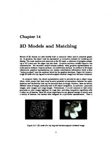
Figure 1 illustrates the proposed method for registering a single image with existing 3D building 2. Registration Method models using extracted edged corner features. It starts by back-projecting the 3D building models to Figure 1 illustrates the proposed method for registering a single image with existing 3D building the image using initial (or atedged later corner steps features. updated) EOPs.byThen with the help ofbuilding the similarity measure, models using extracted It starts back-projecting the 3D models to the image using initial at later steps updated) withmethod. the help of the similarity measure, feature the matching process finds (or corresponding featuresEOPs. usingThen a CGH Based on the matched the EOPs matching process finds corresponding features CGH method. Based As on shown the matched pairs, the of the single image are estimated by ausing leastasquare adjustment. in Figure 1, feature pairs, the EOPs of the single image are estimated by a least square adjustment. As shown in the second and third steps are conducted iteratively to find optimal EOPs until the corresponding Figure 1, the second and third steps are conducted iteratively to find optimal EOPs until the matching pairs do not further improve. The three steps of the proposed method are further discussed corresponding matching pairs do not further improve. The three steps of the proposed method are in the following sub-sections whereatsub-sections the last two stepsthe arelast discussed further discussed in the following whereat two stepstogether. are discussed together.
Figure 1. Flowchart of the proposed model-to-image registration method.
Figure 1. Flowchart of the proposed model-to-image registration method.
Sensors 2016, 16, 932
5 of 20
2.1. Feature Extraction Feature extraction is the first step of the registration task. As previously mentioned, feature selection should consider the properties of the given datasets, the application, and the required accuracy. In this study, we use two different types of features: edged corner features, and context features. An edged corner feature, which consists of a corner point, and the two associated lines that potentially intersect at this point (“arms”), provides local structure information for a building. In building models, it is relatively straightforward to extract this feature because each vertex of a building polygon can be treated as a corner and the connected lines as arms. Note that only rooftop polygons are considered for this. In an image with rich texture information, various corner detectors, and line detectors can be used to extract edged corner features. A context feature is defined as a characteristic spatial relation between two edged corner features selected within an individual roof. This context feature is used to represent global structure information so that more accurate, and robust matching results can be achieved. Section 2.1.1 explains the extraction of edged corner features from an image, and Section 2.1.2 describes the properties of context features. 2.1.1. Edged Corner Feature Extraction from Image Edged corner features from a single image are extracted by three separate steps; (1) extraction of straight lines; (2) extraction of corners, and their arms; and (3) verification. The process starts with the extraction of straight lines from a single image by applying a straight line detector. We use Kovesi’s algorithm, which relies on the calculation of phase congruency to localize, and link edges [26]. Then, corners are extracted by estimating the intersection of the extracted straight lines, considering the proximity with a given distance threshold (Td “ 20 pixels). Afterwards, corner arms are determined by two straight lines used to extract the corner with fixed length (20 pixels). This procedure may produce incorrect corners because the proximity constraint is the only one considered. Thus, the verification process removes incorrectly extracted corners based on geometric and radiometric constraints. As a geometric constraint, the inner angle between two corner arms is calculated, and investigated to remove corners with sharp inner angles. In general, many of building structures appears in regular shapes following orthogonality and parallelism where small acute angles are found to be uncommon. Through this process, incorrectly extracted corners are filtered out by applying a user-defined inner angle threshold (Tθ “ 10˝ ). For the radiometric constraint, we analyze the radiometric values (Digital Number (DN) value or color value) of the left, and right flanking regions (F1L , F1R , F2L , F2R ) of each corner arm with a flanking width (ε) as used in [27]. Figure 2 shows a configuration of a corner, its arms, and the concept of the flanking regions. In a correctly extracted corner, the average DN (or color) difference between F1L and F2R , k F1L ´ F2R k, or between F1R and F2L , k F1R ´ F2L k, is likely to be small, underlining the homogeneity of two regions, while average DN difference between F1L and F2L , k F1L ´ F2L k, or between F1R and F2R , k F1R ´ F2R k, should be large enough to underline the heterogeneity of two regions. Thus, we measure two radiometric properties: the minimum average DN difference value of two neighbor flanking regions for homogeneity measurement, ` ˘ homo “ min k F L ´ F R k, k F R ´ F L k , and the maximum DN difference value of two opposite Dmin 2 2 1 1 ` ˘ hetero “ max k F L ´ F L k, k F R ´ F R k . A corner flanking regions for heterogeneity measurement, Dmax 2 2 1 1 homo than a threshold T is considered an edged corner feature if the corner has a smaller Dmin homo , and if it hetero than a threshold T has a larger Dmax . hetero In order to determine thresholds for two radiometric properties, we assume that the intersection points are generated from both correct corners, and incorrect corners; and the two types of intersection points have different distributions with regards to their radiometric properties. Because there are two cases (correct corner and incorrect corner) for the average DN difference values, we can use the Otsu’s binarization method [28] to automatically determine an appropriate threshold value. The method was originally designed to extract an object from its background for binary image segmentation based on histogram distribution. It calculates the optimum threshold by separating the two classes (foreground and background) in such a way that their intra-class variance is minimal. In our study,
flanking regions ( , , , ) of each corner arm with a flanking width (ε) as used in [27]. Figure 2 shows a configuration of a corner, its arms, and the concept of the flanking regions. In a correctly extracted corner, the average DN (or color) difference between and , ‖ − ‖, or between and , ‖ − ‖, is likely to be small, underlining the homogeneity of two regions, while average DN difference between and , ‖ − ‖, or between and , ‖ − ‖, should Sensorsbe 2016, 16, enough 932 large to underline the heterogeneity of two regions. Thus, we measure two radiometric6 of 20 properties: the minimum average DN difference value of two neighbor flanking regions for (‖ − ‖, ‖ − ‖), and the maximum DN difference homogeneity measurement, = Sensors 2016, 16, 932 6− of 20 is a histogram of homogeneity values (or heterogeneity values) for the entire selection of (‖ points value of two opposite flanking regions for heterogeneity measurement, = generated, the optimal threshold for homogeneity (or heterogeneity) is automatically determined ‖, ‖ and ‖). A corner is considered an edged corner feature if the corner has a smaller − In order to determine thresholds two radiometric that the intersection than abinarization threshold , and if it has afor larger thanproperties, a thresholdwe assume . by Otsu’s method.
points are generated from both correct corners, and incorrect corners; and the two types of intersection points have different distributions with regards to their radiometric properties. Because Arm2 there are two cases (correct corner and incorrect corner) for the average DN difference values, we can use the Otsu’s binarization method [28] to automatically determine an appropriate threshold value. F2R F The method was originally designed to extract an object from its background for binary image segmentation based on histogram distribution. It calculates the optimum threshold by separating the F1 L two classes (foreground and background) in such a way thatArm their intra-class variance is minimal. In 1 F Corner our study, a histogram of homogeneity values (or heterogeneity values) for the entire selection of points is generated,Figure and 2. the optimal for homogeneity (orflanking heterogeneity) Edged cornerthreshold feature (corner and its arms) and regions. is automatically Figure 2. Edged corner feature (corner and its arms) and flanking regions. determined by Otsu’s binarization method. L 2
R 1
2.1.2. Context Features 2.1.2. Context Features While an edged corner feature provides only local structure information about a building corner, While an edged corner feature provides only local structure information about a building corner, context features partly impart global structure information related to the building configuration. context features partly impart global structure information related to the building configuration. Context features edged corner cornerfeatures, features,that thatis,is,four four angles Context featuresare areset setby byselecting selecting any any two two adjacent adjacent edged angles le f t right le f t right (θi ( , θi , , θ j , , θ j , ) between a line (l) connecting the two corners (C and C ), and their arms ) between a line (l) connecting the two corners ( i and ),j and their arms right
le f t
right
(Arm , Arm ) )as inFigure Figure3.3.Note Note angle is determined , i , j , Arm , as shown shown in thatthat eacheach angle is determined by theby ( left i , Arm j therelative relativeline lineconnecting connecting any two corners (l). The context feature, which is invariant under scale, any two corners (l). The context feature, which is invariant under scale, translation, and rotation, similarityin inour ourproposed proposedscore score function (see translation, and rotation,isisused usedtotocalculate calculate contextual contextual similarity function (see Section 2.2.2). Section 2.2.2). Arm right j
Cj right j
left j
Arm
Armileft
left j
ileft iright
Ci
Armiright
Figure 3. 3. Context Context feature. Figure feature.
Similarity Measurementand andMatching Matching 2.2.2.2. Similarity Measurement Similarity measurement matching process place inimage the image after 3D Similarity measurement andand matching process taketake place in the spacespace after the 3Dthe building building are back-projected onto space the image using the collinearity equations with the models are models back-projected onto the image usingspace the collinearity equations with the initial EOPs initial EOPs (or updated EOPs). In order to find reliable and accurate correspondences between (or updated EOPs). In order to find reliable and accurate correspondences between features extracted features extracted from a single image, and building models, we introduce a CGH method where the from a single image, and building models, we introduce a CGH method where the vote counting vote counting scheme of a standard geometric hashing is supplemented by a newly developed scheme of a standard geometric hashing is supplemented by a newly developed similarity score similarity score function. The similarity score function consists of a unary term, and a contextual term. function. The similarity score function consists of a unary term, and a contextual term. The unary term The unary term measures the similarity between edged corner features derived from the image, and measures the similarity between edged corner features derived from the image, and models while models while the contextual term measures the geometric property of context features. In the the contextual term measures the geometric property of context features. In the following sections, following sections, the standard geometric hashing, and its limitations are described (Section 2.2.1), theand standard geometric its limitations are2.2.2). described (Section 2.2.1), and our proposed our proposed CGHhashing, method and is introduced (Section CGH method is introduced (Section 2.2.2). 2.2.1. Geometric Hashing 2.2.1. Geometric Hashing Geometric hashing, a well-known indexing-based approach, is a model-based object recognition Geometric well-known indexing-based approach, is a model-based object recognition technique for hashing, retrievingaobjects in scenes from a constructed database [29]. In geometric hashing, an technique retrieving scenes from a constructed database [29]. and In geometric hashing, object is for represented asobjects a set ofingeometric features such as points, and lines, by its geometric an object is represented as a set of geometric features such as points, and lines, and by its geometric
Sensors 2016, 16, 932
7 of 20
Sensors 2016, 16, 932
7 of 20
relations, which are transformation-invariant under certain transformations. Since only local invariant relations, whichareare transformation-invariant transformations. Since onlyhashing local geometric features used, geometric hashing can under handlecertain partly occluded objects. Geometric invariant geometric features are used, geometric hashing can handle partly occluded objects. consists of two main stages: the pre-processing stage, and the recognition stage. The pre-processing Geometric consists of two main stages: pre-processing stage, andinthe recognition stage. a stage encodes hashing the representation of the objects in athe database, and stores them a hash table. Given The pre-processing stage encodes the representation of the objects in a database, and stores them in set of object points (pk ; k “ 0, . . . , n), a pair of points (pi and p j ) is selected as a base pair (Figure 4a). a hash table. Given a set of object points ( ; = 0, … , ), a pair of points ( and ) is selected as a The base pair is scaled, rotated, and translated into the reference frame. In the reference frame, base pair (Figure 4a). The base pair is scaled, rotated, and translated into the reference frame. In the the magnitude of the base pair equals 1; the midpoint between pi and p j is placed at the origin of the ´ ÝÑ of ¯ the base pair equals 1; the midpoint between reference frame, the magnitude and is placed reference frame.ofThe vector pframe. vector of the The of remaining i p j corresponds at the origin the reference The vector (to a unit ) corresponds to a x-axis. unit vector the x-axis.points The of the model are located in the coordinate frame based on the corresponding base pair (Figure 4b). remaining points of the model are located in the coordinate frame based on the corresponding base Thepair locations (to be used as index) are quantized by a proper bin size and recorded with the form (Figure 4b). The locations (to be used as index) are quantized by a proper bin size and recorded (model pair in base the hash table. Forhash all possible base pairs, allbase entries ofall points are withID, the used form base (model ID,ID) used pair ID) in the table. For all possible pairs, entries similarly recorded in the recorded hash table of points are similarly in(Figure the hash4c). table (Figure 4c). y
p2 p1
p3
p5
p4 p3
p5
p1
p2
-0.5
0.5
x
p4 (a)
(b)
(c)
Figure 4. Geometric Hashing: (a) model points; (b) hashing table with base pair and (c) all hashing Figure 4. Geometric Hashing: (a) model points; (b) hashing table with base pair and (c) all hashing table entries with all base pairs. table entries with all base pairs.
In the subsequent recognition stage, the invariants, which are derived from geometric features subsequent recognition stage, invariants, whichconstructed are derivedhash fromtable geometric inIna the scene, are used as indexing keys to the assess the previously so thatfeatures they canin a scene, are used as indexing keys to assess the previously constructed hash table so that they can abe be matched with the stored models. In a similar way to the preprocessing stage, two points from matched with the models. In a similar theThe preprocessing stage,are twomapped points from set of set of points in stored the scene are selected as the way base to pair. remaining points to theahash points in the are selected the base pair.hash The table remaining points aare mapped to the hash table, table, andscene all entries in the as corresponding bin receive vote. Correspondences are anddetermined all entries in the corresponding hash table bin receive a vote. Correspondences are determined by by a vote counting scheme, producing candidate matches. Although geometric hashingcandidate can solvematches. matching problems of rotated, translated, and partly a vote counting scheme, producing occluded objects, it has some limitations. Thematching first limitation is thatof the methodtranslated, is sensitive and to thepartly bin Although geometric hashing can solve problems rotated, size used for quantization of the hash table. While a large bin size in the hash table cannot separate occluded objects, it has some limitations. The first limitation is that the method is sensitive to the bin close points,ofathe small bintable. size cannot withbin thesize position the point. Secondly, sizebetween used fortwo quantization hash Whiledeal a large in theerror hashoftable cannot separate geometric can produce solutions tothe its vote counting [29]. Although between two hashing close points, a small redundant bin size cannot dealdue with position errorscheme of the point. Secondly, it can significantly candidate hypotheses, verification stepcounting or additional fine[29]. matching step it geometric hashing canreduce produce redundant solutionsa due to its vote scheme Although is required to find optimal matches. Thirdly, geometric hashing has a weakness in cases where theis can significantly reduce candidate hypotheses, a verification step or additional fine matching step scene contains many features of similar shapes at different scales, and rotations. Without any required to find optimal matches. Thirdly, geometric hashing has a weakness in cases where the scene constraints (e.g., position, scale and rotation) based on prior knowledge about the model, geometric contains many features of similar shapes at different scales, and rotations. Without any constraints hashing may produce incorrect matches due to the matching ambiguity. Fourthly, the complexity of (e.g., position, scale and rotation) based on prior knowledge about the model, geometric hashing may processing increases by the number of base pairs, and the number of features in the scene [6]. To produce incorrect matches due to the matching ambiguity. Fourthly, the complexity of processing address these limitations, we enhance the standard geometric hashing by changing the vote counting increases by the number of base pairs, and the number of features in the scene [6]. To address these scheme to a score function, and by adding several constraints such as scale difference of a base, and limitations, we enhance the standard geometric hashing by changing the vote counting scheme to specific selection of bases. a score function, and by adding several constraints such as scale difference of a base, and specific selection of bases. 2.2.2. Context-Based Geometric Hashing (CGH) In this section, we describe the building 2.2.2. Context-Based Geometric Hashing (CGH) model objects and the scene by sets of edged corner features. Edged corner features derived from input building models are used to construct the hash In this section, we describe building objects and the from scenethe bysingle sets of edged table in the pre-processing stagethe while edged model corner features derived image are corner used features. Edged corner features derived from input building models are used to construct theprehash in the recognition stage. Each given building model consists of several planes. Thus, in the table in the pre-processing stage while edged corner features derived from the single image are used in the recognition stage. Each given building model consists of several planes. Thus, in the pre-processing
Sensors 2016, 16, 932
8 of 20
Sensors 2016, 16, 932
8 of 20
stage, we select two edged corner features, which belong to the same plane of the building model as processing we select two edged corner features, which belong to the same plane of the building the base It stage, can Sensorspair. 2016, 16, 932 reduce the complexity of the hashing table, and ensures that the base pair 8 ofretains 20 model as the base pair. It can reduce the complexity of the hashing table, and ensures that the base the spatial information of the plane. The selected base pair is scaled, rotated, and translated to define pair retains thewe spatial information of corner thefeatures, plane. The selected base pair is plane scaled, and processing stage, select two edged corner which belong to the same ofrotated, the building the reference frame. The remaining edged features which belong to the whole building model translated to define the reference frame. The remaining edged corner features which belong to the model as the base pair. canbase reduce theIncomplexity thestandard hashing table, and ensures thatour the base are also transformed withItthe pair. contrast toofthe geometric hashing, hashing whole building model are also transformed with theThe baseselected pair. In contrast to is the standard geometric retains the spatial pair rotated, tablepair contains model IDs, information feature IDs ofofthe theplane. base pair, the scalebase of the basescaled, pair (the rateand of real hashing, our hashing table contains model IDs, feature IDs of the base pair, the scale of the basetopair translated to define the reference frame. The remaining edged corner features which belong the by distance of base pair), an index for member edged corner features, and context features generated (the rate of real distance of base pair), anwith index member corner features, and context whole building model are also transformed thefor base pair. Inedged contrast to the standard geometric combinations with edged corner features. Figure 5corner showsfeatures. an example of5the information to of bethe stored features generated by combinations with edged Figure shows an example hashing, our hashing table contains model IDs, feature IDs of the base pair, the scale of the base pair in a hashing table. information to be stored in a hashing table. (the rate of real distance of base pair), an index for member edged corner features, and context features generated by combinations with edged corner features. Figure 5 shows an example of the p p4 information to be stored in a2 hashing table. p1
p3
p2
p1 p5
p3
p4
(a)
p5
p4
p5
p1
p2
p3
p3
p5
p1 (b) p2
p4 Figure 5. (a) Edged corner features derived from a model, and (b) information to be stored in a Figure 5. (a) Edged corner features derived from a model, and (b) information to be stored in a hashing hashing table (dotted (a)lines represent context features). (b) table (dotted lines represent context features). Figure Edged base corner features derived from a model, (b)toinformation to be stored in a Once5.all(a) possible pairs are set, the recognition stageand tries retrieve corresponding features hashing table (dotted lines represent context features). Once basescore pairsfunction. are set, Two the recognition tries to retrieve features basedall onpossible the designed edged cornerstage features from the imagecorresponding are selected as base
two constraints: scale constraint; and (2) position constraint. Asthe a constraint on selected a scale, as basedpair on with the designed score (1) function. Two edged corner features from image are Once allbase possible base pairs are set, the to recognition stage triespair to retrieve corresponding features only those pairs whose scale is similar the scale of the base in the hash table are considered base pair with two constraints: (1) scale constraint; and (2) position constraint. As a constraint on based on designed score Two edged an corner features from the image areThus, selected asscale base with an the assumption thefunction. initial EOPs scale of the image. if the a scale, only those basethat pairs whose scaleprovide is similarapproximate to the scale of the base pair in the hash table pair with two constraints: (1) scale constraint; and (2) position constraint. As a constraint on a scale, ratio is smaller than a user defined threshold ( = 0.98), the base pair is excluded from the set of are considered with an assumption that the initial EOPs provide an approximate scale of the image. only those base base pairs. pairs whose scale is to the scalethe of the base pair in theof hash tablepair arecan considered possible In addition tosimilar scale constraint, possible positions a base be also Thus, if the scale ratio is smaller than a user defined threshold (T “ 0.98), the base pair is excluded s with an assumption that the initial EOPs an approximate of the image. Thus, if the scale restricted with a proper searching space.provide This searching space canscale be determined by calculating error fromratio the of possible pairs. Inthreshold addition theispossible positions of aofbase isset smaller thanthe a base user defined ( to =scale 0.98),constraint, the pair excluded from the EOPs set propagation with amount of assumed errors (calculated bybase the iterative process) for initial pairpossible can be also restricted with a and proper searching space. This searching canpair be determined base pairs. In addition to scale constraint, the possible positions ofthe a base can be also by (updated EOPs) of the image, the models. These two constraints reducespace matching ambiguity, calculating error propagation with the amount ofselection assumed (calculated iterative process) restricted with a properofsearching space. This space can be determined bythe calculating error and the complexity processing. After thesearching of errors possible base pairsby from the image, all propagation thecorner amount of of assumed errors (calculated by the iterative process) for initial EOPs for initial EOPswith (updated EOPs) the image, and models. These reduce remaining edged features in the image arethe transformed based two on aconstraints selected base pair. the (updated EOPs) the image, and the These constraints reduce the matching ambiguity, Afterwards, theofoptimal are models. determined bytwo comparing similarity score. The process startsfrom matching ambiguity, and thematches complexity of processing. After thea selection of possible base pairs and the complexity of processing. After the selection of possible base pairs from the image, allbase by generating context features from the model, and the image in a reference frame. Given a model the image, all remaining edged corner features in the image are transformed based on a selected remaining edged corner features in the image are transformed based on a selected base pair. that consists of five edged corner features (black color), ten context features can be generated as pair. Afterwards, the optimal matches are determined by comparing a similarity score. The process Afterwards, the optimal are determined by comparing a similarity score. process starts shown in Figure 6. Notematches that all edged corner features derived from the model are The not matched with starts by generating context features from the model, and the image in a reference frame. Given a byedged generating and color). the image in only a reference frame. features, Given a which model cornercontext featuresfeatures derivedfrom fromthe themodel, image (red Thus, edged corner model that consists of five edged corner features (black color), ten context features can be generated have corresponding image corner edged corner features area (n = 4 incan Figure 6), and their that consists of five edged features (blackwithin color),the tensearch context features be generated as as shown in Figurecontext 6. Note that all(medged corner6features derivedare from the model arecalculation not matched corresponding = 6corner in Figure (redderived long-dash)) in the shown in Figure 6. Note features that all edged features from theconsidered model are not matched with withedged edged corner features derived the image (red color). Thus, only edged cornerwhich features, of thecorner similarity scorederived function. features fromfrom the image (red color). Thus, only edged corner features, which have corresponding image edged corner features within the search area (n = 4 in Figure have corresponding image edged corner features within the search area (n = 4 in Figure 6), and their 6), and corresponding their corresponding context (m features (m = 66in Figure 6 (red are long-dash)) in the context features = 6 in Figure (red long-dash)) consideredare in considered the calculation calculation of the similarity score function. of the similarity score function.
Figure 6. Context features to be used for calculating score function.
Figure 6. Context features to be used for calculating score function.
Figure 6. Context features to be used for calculating score function.
Sensors 2016, 16, 932
9 of 20
The newly designed score function consists of a unary term, which measures the position differences of the matched points, and a contextual term, which measures length and angle differences of corresponding context features, as follows: « ff řn řn řn i “1 j“1 C pi, jq i“1 U piq score “ α ˆ w ˆ (1) ` p1 ´ wq ˆ n m where: $ & 0
if
% 1
else
α“
# o f matched f eatures # o f f eatures in the model
ă Tc
(2)
α is an indicator function where the minimum number of features to be matched is determined depending on Tc (Tc “ 0.5, at least 50% of corners in the model should be matched with corners from the image) so that all features of the model do not need to be detected in the image; n and m are the number of matched edged corner features, and context features, respectively; w is a weight value which balances the unary term and the contextual term; in our case, w = 0.5 is heuristically selected: Unary term: The unary term U piq measures the position distance between edged corner features derived from the model, and the image in a reference frame. The position difference k PiM ´ PiI k between an edged corner feature in the model and its corresponding feature in the image is normalized by the distance NiP calculated by the EOP error propagation on the image plane: U piq “
NiP ´ k PiM ´ PiI k
(3)
NiP
Contextual term: This term is designed to measure the similarity between context features in terms of length and four angles. The contextual term is calculated for all context features which are generated from matched edged corner features. For the length difference, k LijM ´ LijI k, the difference between lengths of context features in the model, and in the image is normalized by length NijL of the context M
I
feature in the model. For angle differences, the angle difference k θij k ´ θijk k between the inner angles of a context feature is normalized by Nijθ (Nijθ “ C pi.jq “
π 2 ):
NijL ´ k LijM ´ LijI k NijL
ř4 `
k “1
´
M
I
Nijθ ´ k θij k ´ θijk k 4 ˆ Nijθ
¯ (4)
For each model, a base pair, and its corresponding corners which maximize the score function are selected as optimal matches. Note that if the maximum score is smaller than a certain threshold Tm , the matches are not considered as matched corners. The role of Tm is to determine an optimal subset of accurate matching correspondences for estimating EOP parameters. High Tm values provide a low number of matching correspondences with high accuracy. In contrast, low Tm values increase the number of matching correspondences but they also decrease their accuracy. Once all correspondences are determined, the EOPs of the image are adjusted through space resection using pairs of object coordinates of the existing building models, and newly derived image coordinates from the matching process. Values calculated from the similarity score function are used to weight matched pairs. The process continues until matched pairs do not change. 3. Experimental Results The proposed CGH-based registration method was tested on benchmark datasets over the downtown areas in Toronto (ON, Canada) and Vaihingen in Germany provided by the ISPRS Commission III, WG3/4 [30]. Table 1 shows characteristics of reference building models, which were used to determine EOPs. For the Toronto datasets, two different types of reference building models were prepared by: (1) a manual digitization process conducted by human operators; and (2) using a state-of-the art algorithm [31] from airborne LiDAR point clouds. These two building models were used to investigate their respective effects on the performance of our method (Figure 7). For the
Sensors 2016, 16, 932
10 of 20
Vaihingen datasets, LiDAR-driven building models were automatically generated by [32] and adjusted Sensors 2016, 16, 932 10 of 20 as described in [33] as shown in Figure 8. A total of 16 check points for each dataset, which were Sensors 2016, 16, 932 10 of 20 evenly distributed throughout images, were used to evaluate the accuracy thedataset, EOPs. which adjusted as described in [33] asthe shown in Figure 8. A total of 16 check points forof each adjusted as described in throughout [33] as shown Figure were 8. A total check points for each which were evenly distributed theinimages, usedof to16 evaluate the accuracy ofdataset, the EOPs. Table 1. Characteristics reference building models. were evenly distributed throughout the images,of were used to evaluate the accuracy of the EOPs. Table 1. Characteristics of reference building models.
Dataset Dataset
Reconstruction of # of Table 1.#Characteristics ofDescription reference building models. Method Buildings Planes Reconstruction # of # of Method
LiDAR-driven [31] Manually digitized
Buildings # of 159 159 Buildings 126 126 159
LiDAR-driven [33]
894 126
Planes # of 1560 1560 Planes 1066 1066 1560
894
2619 1066 2619
LiDAR-driven [33]
894
2619
Dataset Toronto Toronto
Reconstruction Manually digitized Manually digitized Method LiDAR-driven [31]
Toronto Vaihingen
Vaihingen
LiDAR-driven [33] LiDAR-driven [31]
Vaihingen
Description
Complex clusters of high-rise buildings Description Complex clusters of high-rise Maximum building height: buildings approximately 290 m Maximum building height: approximately 290 m building shapes ComplexEuropean clusters ofstyle high-rise buildings Typical structures with simple Typical European style structures with simple Maximum building height: approximately 290 building m m. shapes Maximum building height: approximately 32 Maximum building height: approximately 32 m. Typical European style structures with simple building shapes Maximum building height: approximately 32 m.
(a) (a)
(b) (b)
(c) (c)
(d) (d)
Figure 7. Toronto dataset: (a) LiDAR-driven building models reconstructed by [31]; (b) LiDAR-driven Figure 7. Toronto dataset: (a) LiDAR-driven building models reconstructed by [31]; (b) LiDAR-driven Figure 7. models Toronto(blue dataset: (a)and LiDAR-driven reconstructed by [31]; (b) LiDAR-driven building lines) check pointsbuilding (yellow models triangles) back-projected to image; (c) manually building models (blue lines) and check points (yellow triangles) back-projected to image; (c) manually building models (blue lines) and check pointsdigitized (yellow triangles) back-projected to image; manually digitized building models and (d) manually building models back-projected to(c) image. digitized building models and (d) manually digitized building models back-projected to image. digitized building models and (d) manually digitized building models back-projected to image.
(a) (a)
(b) (b)
Figure 8. Vaihingen dataset: (a) LiDAR-driven building models reconstructed by [33] and (b) LiDARFigure building 8. Vaihingen dataset: LiDAR-driven building models reconstructed by [33] and (b) LiDARdriven models (blue(a) lines) and check points (yellow triangles) back-projected to image. Figure 8. Vaihingen dataset: (a) LiDAR-driven building models reconstructed by [33] and driven building models (blue lines) and check points (yellow triangles) back-projected to image. (b) LiDAR-driven building models (blue lines) and check points (yellow triangles) back-projected For the Toronto dataset, various analyses were conducted to evaluate the performance of the to image.
For the Toronto dataset, analyses were conducted evaluate the performance the proposed registration methodvarious in detail. From the aerial image, atototal of 90,951 straight linesofwere proposed and registration method in detail. aerialby image, a total any of 90,951 straightlines linesfound were extracted 258,486 intersection pointsFrom were the derived intersecting two straight extracted and 258,486 intersection points were derived by intersecting any two straight lines found
Sensors 2016, 16, 932
11 of 20
For the Toronto dataset, various analyses were conducted to evaluate the performance of the Sensors 2016, 16, 932 11 ofwere 20 proposed registration method in detail. From the aerial image, a total of 90,951 straight lines extracted and 258,486 intersection points were derived by intersecting any two straight lines found within 20 pixels of proximity constraint. Out of these, 57,767 intersection points were selected as within 20 pixels of proximity constraint. Out of these, 57,767 intersection points were selected as edged corner features following the removal of 15%, and 60% of intersection points using geometric edged corner features following the removal of 15%, and 60% of intersection points using geometric constraint ( = 10°), and radiometric constraints ( = 26, and = 55), respectively (Table 2). constraint (Tθ “ 10˝ ), and radiometric constraints (Thomo “ 26, and Thetero “ 55), respectively (Table 2). The and were automatically determined by Otsu’s binarization method. Figure 9 The Thomo and Thetero were automatically determined by Otsu’s binarization method. Figure 9 shows shows edged corner features extracted from the aerial image. As many of the intersection points are edged cornertofeatures extracted from the image. As many of method the intersection arecorners not likely not likely be corners, the majority of aerial them were removed. The correctlypoints detected to and be corners, the majority of them were removed. The method correctly detected corners and arms in most cases even though some corners were visually difficult to detect due to theirarms low in most cases even though some corners were visually difficult to detect due to their low contrasts. contrasts.
(a)
(b) Figure 9. Edged corner features from image: (a) straight lines (red) and (b) edged corner features Figure 9. Edged corner features from image: (a) straight lines (red) and (b) edged corner features (blue). (blue).
Table 2. Extracted features and matched features for the Toronto dataset. Table 2. Extracted features and matched features for the Toronto dataset. Image Image
# of extracted features # of extracted features # of matched features # of matched features
Intersections Intersections
Corners Corners
258,486 258,486 -
57,767 57,767 -
Existing Building Models Existing Building Models Manually Digitized LiDAR-Driven Manually Digitized LiDAR-Driven Building Models Models Building Models Building Building Models 8895 7757 6938895 381 7757 693 381
After the existing building models were back-projected onto the image using error-contained After the existing building models werefrom back-projected image models using error-contained EOPs, edged corner features were extracted the verticesonto of thethe building in the image EOPs, corner were extracted the vertices the used building models in building the image spaceedged (Figure 10). Itfeatures should be noted that twofrom different datasetsofwere as the existing space (Figure 10). It should notedextracted that twofrom different datasetsbuilding were used as the existing building models. Some edged cornerbe features both existing models were not observed models. Some due edged corner features extracted frombuilding both existing models notfeatures, observed in the image to occlusions caused by neighbor planes.building Also, some edgedwere corner those extracted caused from LiDAR-driven building planes. models,Also, do not match with the edged in in theparticular image due to occlusions by neighbor building some edged corner features, features extracted from fromLiDAR-driven the image due to modeling by irregular in corner particular those extracted building models,errors do notcaused match with the edgedpoint corner distribution, occlusions andimage the reconstruction mechanism. correspondences between edged features extracted from the due to modeling errors Thus, caused by irregular point distribution, corner features the imagemechanism. and from the existing building models are edged likely corner to be partly occlusions and thefrom reconstruction Thus, correspondences between features established. from the image and from the existing building models are likely to be partly established. The proposed CGHmethod methodwas wasapplied applied to to find derived from The proposed CGH find correspondences correspondencesbetween betweenfeatures features derived from the image and from existing building models. When manually digitized building models are used as as the image and from existing building models. When manually digitized building models are used building models, a total of 693 edged corner features (7.8% of edged corner features extracted from the entire building models) were matched using the parameters given in Table 3.
Sensors 2016, 16, 932
12 of 20
building models, a total of 693 edged corner features (7.8% of edged corner features extracted from the entire2016, building Sensors 16, 932 models) were matched using the parameters given in Table 3. 12 of 20
(a)
(b)
Figure 10. Features from existing building models: (a) manually digitized building models and their Figure 10. Features from existing building models: (a) manually digitized building models and their edged corner features and (b) LiDAR-driven building models and their edged corner features. edged corner features and (b) LiDAR-driven building models and their edged corner features.
It is noted that only models whose vertices were greater than were considered to find It is noted that only models whose vertices were greater than Tc were considered to find possible possible building matches. For LiDAR-driven building models, only 381 edged corner features (4.9% building matches. For LiDAR-driven building models, only 381 edged corner features (4.9% from from the entire building models) were matched (Table 2). It is noted that the number of matched the entire building models) were matched (Table 2). It is noted that the number of matched edged edged corner features is influenced by the quality of the existing building models, and thresholds corner features is influenced by the quality of the existing building models, and thresholds used, Tm in used, in particular. As shown in Table 2, more edged corner features are matched when manually particular. As shown in Table 2, more edged corner features are matched when manually digitized digitized building models were used as the existing building models than when LiDAR-driven building models were used as the existing building models than when LiDAR-driven building models building models were used. If is set as a small value, the number of matched edged corner were used. If Tm is set as a small value, the number of matched edged corner features increases, but this features increases, but this increases the risk it may contain a large number of incorrect matched increases the risk it may contain a large number of incorrect matched edged corner features. The effect edged corner features. The effect on the will be discussed in detail later. on the Tm will be discussed in detail later. Table 3. Parameter setting. Table 3. Parameter setting.
Feature Extraction
Geometric Hashing
Feature Extraction Thomo 20 pixel Td 10° Tθ automatic 20 pixel
10˝
automatic
Geometric Hashing Thetero automatic automatic
Ts 0.98 0.98
Tp T50% c automatic automatic 50%
Tm0.6 0.6
Based on matched edged corner features, EOPs for the image were calculated by applying the Based on matched edged corner features, EOPs for the image were calculated the by applying the least least square method based on co-linearity equations. For qualitative assessment, existing models square method based For qualitative assessment, modelsbackwere were back-projected to on theco-linearity image withequations. refined EOPs. Each column of Figuresthe 11 existing and 12 shows back-projected to the imagewith with error-contained refined EOPs. Each column of Figuresedged 11 andcorner 12 shows back-projected projected building models EOPs (a), matched features (b), and building models with error-contained (a),EOPs matched features (b), andofback-projected back-projected building models with EOPs refined (c). edged In thecorner figures, boundaries the existing buildingmodels modelsare with refined EOPs In the boundaries figures, boundaries of thewith existing building building well matched to (c). building in the image refined EOPs. models are wellInmatched to building boundaries the image EOPs. error (RMSE) of check points our quantitative evaluation, weinassessed thewith rootrefined mean square In our quantitative evaluation, we assessed root(Table mean4). square error (RMSE) of check points back-projected onto the image space using refinedthe EOPs When reference building models back-projected the image space using the refined EOPs (Table When reference building were used as theonto existing building models, results show that4).the average difference in x models and y were usedare as−0.27 the existing models, the results showofthat theand average in x and y directions and 0.33building pixels, respectively, with RMSE ±0.68 ±0.71 difference pixels, respectively. directions ´0.27 and 0.33 pixels, respectively, RMSE ˘0.68 and ˘0.71 pixels, in respectively. The results are with LiDAR-driven buildings modelswith show thatofthe average differences x and y The results buildings models showand that±0.89 the average differences in x and y directions arewith −1.03LiDAR-driven and 1.93 pixels, with RMSE of ±0.95 pixels, respectively. Although directions arebuilding ´1.03 and 1.93 pixels, with of ˘0.95 ˘0.89 pixels, Although LiDAR-driven models are used, theRMSE accuracy of theand EOPs is less than 2respectively. pixels in image space LiDAR-driven 30 building models sample are used, the accuracy ofConsidering the EOPs is less 2 pixels in image space (approximately cm in ground distance (GSD)). that than the point space (resolution) 30 cm in ground sample distance Considering thatprovide the point space (resolution) of(approximately the input airborne LiDAR dataset is larger than (GSD)). 0.3 m, the refined EOPs a greater accuracy of engineering the input airborne LiDAR dataset is larger than 0.3 m, the refined EOPs provide a greater accuracy for applications. for engineering applications.
Sensors 2016, 16, 932
13 of 20
Sensors 2016, 16, 932
(a)
13 of 20
(b)
(c)
Figure 11. Manually digitized building models: (a) with error-contained EOPs; (b) matching relations Figure 11. Manually digitized building models: (a) with error-contained EOPs; (b) matching relations (purple) between edged corner features extracted from the image (blue) and from the models (cyan), (purple) between edged corner features extracted from the image (blue) and from the models (cyan), and (c) with refined EOPs. and (c) with refined EOPs.
Sensors 2016, 16, 932
14 of 20
Sensors 2016, 16, 932
14 of 20
(a)
(b)
(c)
Figure 12. LiDAR-driven building models: (a) with error-contained EOPs; (b) matching relations
Figure 12. LiDAR-driven building models: (a) with error-contained EOPs; (b) matching relations (purple) between edged corner features extracted from the image (blue) and from the models (cyan), (purple) between edged corner features extracted from the image (blue) and from the models (cyan), and (c) with refined EOPs. and (c) with refined EOPs. Table 4. Quantitative assessment with check points (unit: pixel).
Table 4. Quantitative assessment with check points (unit: pixel).
Error-Contained Initial EOPs Error-Contained InitialRMSE EOPs Ave.
Refined EOPs with Manually Refined EOPs with LiDARDigitized Building Models Driven Building Models Refined EOPs with Manually Refined EOPs with Ave. RMSE Ave. RMSE Digitized Building Models LiDAR-Driven Building Models x y x y x y x y x y x y Ave. RMSE Ave. RMSE Ave. RMSE 20.51 −24.81 ±6.64 ±8.22 −0.27 0.33 ±0.68 ±0.71 −1.03 1.93 ±0.95 ±0.89 x y x y x y x y x y x y 20.51 ´24.81 ˘6.64 ˘8.22 ´0.27 0.33 ˘0.68 ˘0.71 ´1.03 1.93 ˘0.95 ˘0.89
Sensors 2016, 16, 932 Sensors 2016, 16, 932
15 of 20 15 of 20
errordistribution distributionofof check points is illustrated in Figure Thedistributions error distributions The error 16 16 check points is illustrated in Figure 13. The13. error showed showed that the interquartile range (IQR) for bothdigitized manually digitized and LiDAR-driven building that the interquartile range (IQR) for both manually and LiDAR-driven building models were models1.5 were under 1.5maximum pixels. Theerror maximum value for LiDAR-driven models was however 1 pixel under pixels. The valueerror for LiDAR-driven models was however 1 pixel greater greater for manually than forthan manually digitizeddigitized models.models.
(a)
(b)
Figure 13. Error distributions for 16 check points when (a) manually digitized building models are Figure 13. Error distributions for 16 check points when (a) manually digitized building models are used and (b) LiDAR-driven building models are used. used and (b) LiDAR-driven building models are used.
In this study, threshold, has an effect on the accuracy of the EOPs. In order to evaluate the In this study, threshold, Tm has an effect on the accuracy of the EOPs. In order to evaluate the effect effect of , we estimated the matched number of edged corner features, and calculated the average of Tm , we estimated the matched number of edged corner features, and calculated the average error and error and the RMSE of the check points with different values of . As shown in Table 5, the number the RMSE of the check points with different values of Tm . As shown in Table 5, the number of matched of matched features is inversely proportional to the value of , regardless of which existing building features is inversely proportional to the value of Tm , regardless of which existing building models are models are used. However, the effect of on the accuracy is not the same for both building models. used. However, the effect of Tm on the accuracy is not the same for both building models. We observed We observed affects the matching accuracy of digitized building models less than it does for Tm affects the matching accuracy of digitized building models less than it does for LiDAR-driven LiDAR-driven building models. Furthermore, the matching accuracy tends to get worse with very building models. Furthermore, the matching accuracy tends to get worse with very low or high Tm low or high values. The latter can be explained by the low number of matched features, giving values. The latter can be explained by the low number of matched features, giving us insufficient us insufficient data to accurately adjust the EOPs of the image. In the other case, if a low value is data to accurately adjust the EOPs of the image. In the other case, if a low Tm value is selected, the selected, the number of matched features increases, but so does the number of incorrect matches if number of matched features increases, but so does the number of incorrect matches if the building the building models are inaccurate. Thus, we can observe that LiDAR-driven building models, models are inaccurate. Thus, we can observe that LiDAR-driven building models, reconstructed with reconstructed with relatively lower accuracy compared to the manually digitized models, produced relatively lower accuracy compared to the manually digitized models, produced more sensitive results more sensitive results in the matching accuracy according to . In contrast, the matching accuracy in the matching accuracy according to Tm . In contrast, the matching accuracy of the manually digitized of the manually digitized building models remains high because of high model accuracy. In summary, building models remains high because of high model accuracy. In summary, a higher accuracy of the a higher accuracy of the building models can lead to a higher EOP accuracy, while the value of building models can lead to a higher EOP accuracy, while the value of Tm should be determined by should be determined by balancing the ratio of correct matched features and incorrect matched balancing the ratio of correct matched features and incorrect matched features. features. Table 5. Effect for Tm (unit: pixel). Table 5. Effect for (unit: pixel). Manually Digitized Building Models Manually Digitized Building Models Tm Tm 0.9 0.9 0.8 0.8 0.7 0.7 0.6 0.5 0.6 0.4 0.5 0.3 0.4 0.2 0.3 0.1 0.2
0.1
# of# of Matched Matched Features Features 67 67 268 268 505 505 693 766693 796766 800796 800800 800800
800
x
x
0.38 0.38 0.00 0.00 −0.20 ´0.20 −0.27 ´0.27 −0.22 ´0.22 0.25 0.25 0.00 0.00 0.00 0.00 0.00
0.00
y
y
## of of Matched Matched Features Features 9 9 98 98 273 273 381 381 438 438 499 499 502 502 502 502 502
RMSE RMSE
Ave. Ave.
y
x
x
LiDAR-Driven Building LiDAR-Driven BuildingModels Models
y
0.78 0.78 0.84 0.84 0.31 0.31 0.33 0.33 0.21 0.21 −0.08 ´0.08 −0.09 ´0.09 −0.09 ´0.09 −0.09
±0.43 ˘0.43 ±0.81 ˘0.81 ±0.95 ˘0.95 ±0.68 ˘0.68 ±0.81 ˘0.81 ±1.06 ˘1.06 ±0.88 ˘0.88 ±0.88 ˘0.88 ±0.88
±0.42 ˘0.42 ±0.97 ˘0.97 ±1.08 ˘1.08 ±0.71 ˘0.71 ±0.66 ˘0.66 ±0.75 ˘0.75 ±0.71 ˘0.71 ±0.71 ˘0.71 ±0.71
´0.09
˘0.88
˘0.71
502
RMSE RMSE
Ave. Ave.
xx 0.49
0.49 −1.09 ´1.09 −1.58 ´1.58 −1.03 ´1.03 −0.43 ´0.43 1.21 1.21 1.37 1.37 1.37 1.37 1.37 1.37
yy −1.93
´1.93 1.22 1.22 1.56 1.56 1.93 1.93 3.26 3.26 2.15 2.15 2.19 2.19 2.19 2.19 2.19 2.19
xx ±7.39
˘7.39 ±1.53 ˘1.53 ±0.68 ˘0.68 ±0.95 ˘0.95 ±2.61 ˘2.61 ±3.06 ˘3.06 ±3.12 ˘3.12 ±3.12 ˘3.12 ±3.12 ˘3.12
y y ±6.99
˘6.99 ±1.52 ˘1.52 ±0.61 ˘0.61 ±0.89 ˘0.89 ±3.52 ˘3.52 ±3.66 ˘3.66 ±3.93 ˘3.93 ±3.93 ˘3.93 ±3.93 ˘3.93
In order to evaluate the effect on context feature, we set weight parameter w in score function (Equation (1)) as 1 and 0.5, respectively, and then compared the results. When w = 1, the score function considers only the unary term without the effect of the contextual term so that the contextual force is ignored. As shown in Table 6, the results show that registration with only unary terms causes
Sensors 2016, 16, 932
16 of 20
In order to evaluate the effect on context feature, we set weight parameter w in score function (Equation (1)) as 1 and 0.5, respectively, and then compared the results. When w = 1, the score function considers only the unary term without the effect of the contextual term so that the contextual force Sensors 2016, 16, 932 16 of 20 is ignored. As shown in Table 6, the results show that registration with only unary terms causes considerably considerablylow lowaccuracy accuracyininboth bothcases. cases.In Inparticular, particular,with withLiDAR-driven LiDAR-drivenmodels, models,the theaccuracy accuracyisis heavily These results indicate that the context featuresfeatures has a positive on resolving heavilyaffected. affected. These results indicate thatuse theofuse of context has a effect positive effect on the matching ambiguity and thus improving the EOP accuracy by reinforcing contextual force. resolving the matching ambiguity and thus improving the EOP accuracy by reinforcing contextual
force.
Table 6. Effect of context features (unit: pixel).
Table 6. Effect of context features (unit: pixel). LiDAR-Driven Building Models
Manually Digitized Building Models
Unary term only (w = 1) Unary term only (w = 1) Unary Unaryterm termand and contextual contextualterm term(w (w==0.5) 0.5)
Manually Digitized Ave. Building Models RMSE # of Matched Ave. #Features of Matched x y x RMSE y Features x y x y 542 ´0.67 ´0.39 ˘1.56 ˘1.84 542 −0.67 −0.39 ±1.56 ±1.84
693 693
´0.27 −0.27
0.33 0.33
˘0.68 ±0.68
˘0.71 ±0.71
LiDAR-Driven Ave.Building Models RMSE # of Matched Ave. # Features of Matched x y x RMSE y Features x y x y 361 5.98 1.17 ˘7.72 ˘5.31 361 5.98 1.17 ±7.72 ±5.31
381 381
´1.03 −1.03
1.93 1.93 ˘0.95 ±0.95 ˘0.89 ±0.89
We Wealso alsoanalyzed analyzedvarious variousimpacts impactsofoferrors errorsinininitial initialEOPs EOPson onthe thematching matchingaccuracy accuracyby byadding adding different levels of errors to evaluate our proposed method. Each parameter of the EOPs leads different levels of errors to evaluate our proposed method. Each parameter of the EOPs leadstoto different differentbehaviors behaviorsfrom fromback-projected back-projectedbuilding building models: models: X0 and andY0 parameters parametersare arerelated relatedtotothe the translation back-projected building models; Z0 is related to scale; and ϕ cause shape distortion; translationofof back-projected building models; is related toωscale; and cause shape 0 0 κdistortion; (Figure 14). In (Figure order to14). assess the effects on translation scale, errorsand ranging is related to rotation In order to assess the effectsand on translation scale, 0 is related to rotation from 0 mranging to 25 mfrom were 0added position parameters. assess the shape distortion andthe rotation errors m toto25three m were added to three To position parameters. To assess shape effects, errors 0˝ to 2.5˝ ranging were added rotation parameters. 15parameters. shows the distortion andranging rotationfrom effects, errors fromto0°three to 2.5° were added to threeFigure rotation accuracies the refined EOPs with levelEOPs of errors each EOP parameter. of Figure 15 of shows the accuracies of different the refined withfor different level of errors Regardless for each EOP errors in the initial EOPs,ofRMSE 2 pixels for manually building and RMSE parameter. Regardless errorsofinunder the initial EOPs, RMSE of digitized under 2 pixels formodels, manually digitized ofbuilding under 3models, pixels for were achieved. The resultswere indicate that the andLiDAR-driven RMSE of underbuilding 3 pixels models for LiDAR-driven building models achieved. The accuracy of the refined EOPs was less affected byEOPs the amount ofaffected initial EOPs errors. Thisofisinitial due toEOPs the results indicate that the accuracy of the refined was less by the amount fact thatThis the EOPs to that the optimum errors. is dueconverge to the fact the EOPs solution convergeiteratively. to the optimum solution iteratively.
(a)
(b)
(c)
(d)
(e)
(f)
Figure 14. The behaviors caused by errors for EOP parameters: (a) 0 ; (b) 0 ; (c) 0 ; (d) 0 ; (e) ; Figure 14. The behaviors caused by errors for EOP parameters: (a) X0 ; (b) Y0 ; (c) Z0 ; (d) ω0 ; (e) ϕ0 ; and0 and (f) 0 . (f) κ0 .
In order to evaluate the robustness of the proposed registration method, the algorithm was In order to evaluate the robustness of the proposed registration method, the algorithm was applied applied to the Vaihingen dataset. A total of 31,072 edged corner features from the image and 11,812 to the Vaihingen dataset. A total of 31,072 edged corner features from the image and 11,812 edged edged corner features from the existing building models were extracted using the parameters set in corner features from the existing building models were extracted using the parameters set in Table 3. Table 3. A total of 379 edged corner features were matched by the CGH method where was A total of 379 edged corner features were matched by the CGH method where Tm was heuristically set heuristically set as 0.7, and other parameters were set by Table 3. The results of the extracted and as 0.7, and other parameters were set by Table 3. The results of the extracted and matched features are matched features are summarized in Table 7. Sixteen check points were evaluated for error-contained summarized in Table 7. Sixteen check points were evaluated for error-contained EOPs and refined EOPs and refined EOPs. The accuracies of the check points with refined EOPs show that the average EOPs. The accuracies of the check points with refined EOPs show that the average difference for x difference for x and y directions are 0.67 and 0.91 pixels with RMSE of ±1.25 and ±1.49 pixels respectively (Table 8). A summary of the error distribution for the 16 check points is presented in Figure 16. The results suggest that the proposed registration method can achieve accurate and robust matching results even though building models with different error types were used for the registration of a single image.
Sensors 2016, 16, 932
17 of 20
and y directions are 0.67 and 0.91 pixels with RMSE of ˘1.25 and ˘1.49 pixels respectively (Table 8). A summary of the error distribution for the 16 check points is presented in Figure 16. The results suggest that the proposed registration method can achieve accurate and robust matching results even though Sensors building 2016, 16, 932models with different error types were used for the registration of a single image. 17 of 20 With manually digitized building models
With LiDAR-driven building models
(a)
(b)
(c)
(d) Figure 15. The impacts of errors in initial EOPs: (a) 0 and 0 ; (b) 0 ; (c) 0 and 0 ; and (d) 0 . Figure 15. The impacts of errors in initial EOPs: (a) X0 and Y0 ; (b) Z0 ; (c) ω0 and ϕ0 ; and (d) κ0 . Table 7. Extracted features and matched features (the Vaihingen dataset). Table 7. Extracted features and matched features (the Vaihingen dataset). Model Image Straight Lines Intersections Edged Corners EdgedModel Corners Image # of extracted features 276,109 181,200 31,072 11,812 Intersections Edged Corners Edged Corners Straight Lines # of matched features 379 379 # of extracted features 276,109 181,200 31,072 11,812 # of matched 379 dataset, unit: pixel). 379 Table 8.features Quantitative assessment with check points (the Vaihingen With Refined EOPs With Error-Contained Initial EOPsassessment with check points (the Vaihingen dataset, unit: pixel). Table 8. Quantitative Unary Term Only (w = 1) Unary Term and Contextual Term (w = 0.5) Ave. RMSE Ave. RMSE Ave. RMSE With Refined x y x y x y x y x EOPs y x y With Error-Contained Initial EOPs 22.92 −19.06 ±2.28 ±3.90 −1.32 ±2.45 0.67Term and 0.91 ±1.25 ±1.49 Unary−0.35 Term Only (w = 1) ±2.93 Unary Contextual Term (w = 0.5)
Ave. x 22.92
y ´19.06
RMSE x ˘2.28
y ˘3.90
Ave. x ´1.32
y ´0.35
RMSE x ˘2.45
y ˘2.93
Ave. x 0.67
RMSE y 0.91
x ˘1.25
y ˘1.49
Sensors 2016, 16, 932 Sensors 2016, 16, 932
18 of 20 18 of 20
Figure 16. Error of the the 16 16 check check points points for for the the Vaihingen Vaihingen dataset. dataset. Figure 16. Error distribution distribution of
4. Discussion 4. Discussion In this this paper, paper, we we proposed proposed aa new new model-to-image model-to-image registration registration method method which which can can align align aa single single In image with 3D building models. Edged corner features, represented by a corner and its associated image with 3D building models. Edged corner features, represented by a corner and its associated edges, and and context context features features are are proposed proposed as as the the matching matching features. features. Edged corner features features are are edges, Edged corner extracted from from the the image image by by calculating calculating the the intersection intersection of of two two neighboring neighboring straight straight lines, lines, and and extracted verified using similarity measurement, andand matching, the verified using geometric geometricand andradiometric radiometricproperties. properties.ForFor similarity measurement, matching, CGH method waswas proposed to to compensate forforthe hashing the CGH method proposed compensate thelimitations limitationsofofthe the standard standard geometric geometric hashing method. The qualitative assessment showed that the boundaries of the existing building models, method. The qualitative assessment showed that the boundaries of the existing building models, back-projected by refined EOPs, are well aligned with boundary lines from the image. Meanwhile, back-projected by refined EOPs, are well aligned with boundary lines from the image. Meanwhile, the quantitative quantitativeassessment assessmentshowed showed that both manually digitized building models, and LiDARthe that both manually digitized building models, and LiDAR-driven driven building models can be used to evaluate the EOPs of a single image with acceptable and building models can be used to evaluate the EOPs of a single image with acceptable and reliable reliable accuracy. More specifically, experimental results are summarized as follows: accuracy. More specifically, experimental results are summarized as follows: ‚
The quality of building models directly affects the accuracy of EOPs. When manually digitized The quality of building models directly affects the accuracy of EOPs. When manually digitized building models were used, the proposed registration method accurately and reliably achieved building models were used, the proposed registration method accurately and reliably achieved the EOPs regardless of threshold and assumed error. However, if building models contain more the EOPs regardless of threshold and assumed error. However, if building models contain more modeling errors, the accuracy of EOPs is reduced, which are more susceptible to threshold, and modeling errors, the accuracy of EOPs is reduced, which are more susceptible to threshold, and assumed errors. assumed errors. Contextual features employed in geometric hashing enhances matching performance. This is ‚ Contextual features employed in geometric hashing enhances matching performance. This is because contextual values provide information about the relation between edged corner because contextual values provide information about the relation between edged corner features, features, characterizing geometric properties of individual roof polygon. In particular, the use characterizing geometric properties of individual roof polygon. In particular, the use of context of context features, which provide global information of building models, that is at larger scale features, which provide global information of building models, that is at larger scale (object-level) (object-level) than at using single corners only (point-level), plays a significant role in our than at using single corners only (point-level), plays a significant role in our enhanced geometric enhanced geometric hashing method, and making our matching performance more robust to hashing method, and making our matching performance more robust to errors involved in errors involved in building models used. building models used. The proposed method can iteratively recover the EOPs of a single image in spite of considerable ‚ The proposed method can iteratively recover the EOPs of a single image in spite of considerable error in their initial values, which exceed error amounts permitted in commercial aerial image error in their initial values, which exceed error amounts permitted in commercial aerial acquisition. image acquisition. As future work, we will extend the proposed method to arbitrarily acquired images (e.g., UAV As future work, camera we will images). extend the proposed method to arbitrarily acquired images (e.g., UAV images, and security images, and security camera images). Acknowledgments: This research was funded by the Natural Sciences and Engineering Research Council of Acknowledgments: This research data was set funded by the Natural Engineering Research Council of Canada (NSERC). The Vaihingen was provided by theSciences Germanand Society for Photogrammetry, Remote Canada (NSERC). The Vaihingen data set was provided by the German Society for Photogrammetry, Remote Sensing and andGeoinformation Geoinformation (DGPF) The authors like to acknowledge the of provision of the Sensing (DGPF) [34].[34]. The authors wouldwould like to acknowledge the provision the Downtown Downtown data set by Teledyne Inc.,Solutions First BaseInc., Solutions Inc., at York University, Toronto dataToronto set by Teledyne Optech Inc.,Optech First Base GeoICT LabGeoICT at YorkLab University, and ISPRS WG and III/4. ISPRS WG III/4. Author Contributions: J.J. and G.S. conceived and designed the experiments; K.B. and A.W. contributed with the Author Contributions: J.J. and G.S. conceived and designed the experiments; K.B. and A.W. contributed with experimental work and data analysis; C.A. and M.K. dedicated their valuable suggestions and comments on the the experimental work and analysis; and M.K. dedicatedtotheir valuableand suggestions comments on interpretation of results anddata on the paper; C.A. all authors contributed the writing editing ofand the paper. the interpretation of results and on the paper; all authors contributed to the writing and editing of the paper.
Sensors 2016, 16, 932
19 of 20
Conflicts of Interest: The authors declare no conflict of interest.
References 1.
2. 3. 4. 5. 6.
7. 8. 9. 10. 11.
12.
13.
14.
15.
16.
17.
18. 19.
Sohn, G.; Jung, J.; Jwa, Y.; Armenakis, C. Sequential modeling of building rooftops by integrating airborne LiDAR data and optical imagery: Preliminary results. In Proceedings of the VCM 2013—The ISPRS Workshop on 3D Virtual City Modeling, Regina, SK, Canada, 28–31 May 2013; pp. 27–33. Brown, L.G. A survey of image registration techniques. ACM Comput. Surv. 1992, 24, 326–376. [CrossRef] Zitova, B.; Flusser, J. Image registration method: A survey. Image Vis. Comput. 2003, 21, 977–1000. [CrossRef] Fonseca, L.M.G.; Manjunath, B.S. Registration techniques for multisensor remotely sensed imagery. Photogramm. Eng. Remote Sens. 1996, 62, 1049–1056. Habib, A.; Ghanma, M.; Morgan, M.; Al-Ruzouq, R. Photogrammetric and LiDAR data registration using linear features. Photogramm. Eng. Remote Sens. 2005, 71, 699–707. [CrossRef] Lamdan, Y.; Wolfson, H. Geometric hashing: A general and efficient model-based recognition scheme. In Proceedings of the Second International Conference on Computer Vision (ICCV’88), Tarpon Springs, FL, USA, 5–8 December 1988; pp. 238–249. Mishra, R.K.; Zhang, Y. A review of optical imagery and airborne LiDAR data registration methods. Open Remote Sens. J. 2012, 5, 54–63. [CrossRef] Kaneko, S.; Satoh, Y.; Igarashi, S. Using selective correlation coefficient for robust image registration. Pattern Recognit. 2003, 36, 1165–1173. [CrossRef] Castro, E.D.; Morandi, C. Registration of translated and rotated images using finite Fourier transform. IEEE Trans. Pattern Anal. Mach. Intell. 1987, 9, 700–703. [CrossRef] [PubMed] Viola, P.; Wells, W.M. Alignment by maximization of mutual information. Int. J. Comput. Vis. 1997, 24, 137–154. [CrossRef] Wunsch, P.; Hirzinger, G. Registration of CAD-models to images by iterative inverse perspective matching. In Proceedings of the 13th International Conference on Pattern Recognition (ICPR’96), Vienna, Austria, 25–29 August 1996. Avbelj, J.; Iwaszczuk, D.; Stilla, U. Matching of 3D wire-frame building models with image features from infrared video sequences taken by helicopters or UAVs. In Proceedings of the Proceedings of PCV 2010—Photogrammetric Computer Vision and Image Analysis, Paris, France, 1–3 September 2010; Volume 38, pp. 149–154. Frueh, C.; Russell, S.; Zakhor, A. Automated texture mapping of 3D city models with oblique aerial imagery. In Proceedings of the 2nd International Symposium on 3D Data Processing, Visualization and Transmission, Thessaloniki, Greece, 6–9 September 2004. Hsu, S.; Samarasekera, S.; Kumar, R.; Sawhney, H.S. Pose estimation, model refinement, and enhanced visualization using video. In Proceedings of the 2000 IEEE Conference on Computer Society Computer Vision and Pattern Recognition, Hilton Head, SC, USA, 13–15 June 2000; pp. 488–495. Eugster, H.; Neibiker, S. Real-time georegistration of video streams from mini or micro UAS using digital 3D city models. In Proceedings of the 6th International Symposium on Mobile Mapping Technology, Presidente Prudente, Brazil, 21–24 July 2009. Avbelj, J.; Iwaszczuk, D.; Müller, R.; Reinartz, P.; Stilla, U. Coregistration refinement of hyperspectral images and DSM: An object-based approach using spectral information. ISPRS J. Photogramm. Remote Sens. 2015, 100, 23–34. [CrossRef] Iwaszczuk, D.; Helmholz, P.; Belton, D.; Stilla, U. Model-to-image registration and automatic texture mapping using a video sequence taken by a mini UAV. In Proceedings of the International Archives of the Photogrammetry, Remote Sensing and Spatial Information Sciences, Hannover, Germany, 21–24 May 2013; Volume XL-1/W1. Yang, B.; Chen, C. Automatic registration of UAV-borne sequent images and LiDAR data. ISPRS J. Photogramm. Remote Sens. 2015, 101, 262–274. [CrossRef] Persad, R.A.; Armenakis, C.; Sohn, G. Automatic co-registration of pan-tilt-zoom (PTZ) video images with 3D wireframe models. Photogramm. Eng. Remote Sens. 2015, 81, 847–859. [CrossRef]
Sensors 2016, 16, 932
20.
21. 22. 23. 24.
25.
26.
27. 28. 29. 30.
31.
32.
33.
34.
20 of 20
Tian, Y.; Gerke, M.; Vosselman, G.; Zhu, Q. Automatic edge matching across an image sequence based on reliable points. In Proceedings of the International Archives of the Photogrammetry, Remote Sensing and Spatial Information Science, Beijing, China, 3–11 July 2008; Volume 37, pp. 657–662. Lowe, D.G. Three-dimensional object recognition from single two-dimensional images. Artif. Intell. 1987, 31, 355–395. [CrossRef] Khoshelham, K.; Li, Z. A model-based approach to semi-automated reconstruction of buildings from aerial images. Photogramm. Record 2004, 19, 342–359. [CrossRef] Vosselman, G.; Veldhuis, H. Mapping by dragging and fitting of wire-frame models. Photogramm. Eng. Remote Sens. 1999, 65, 769–776. Ding, M.; Lyngbaek, K.; Zakhor, A. Automatic registration of aerial imagery with untextured 3D LiDAR models. In Proceedings of the IEEE Conference on Computer Vision and Pattern Recognition, Anchorage, AK, USA, 24–26 June 2008. Wang, L.; Neumann, U. A robust approach for automatic registration of aerial images with untextured aerial LiDAR data. In Proceedings of the IEEE Conference on Computer Vision and Pattern Recognition (CVPR’09), Miami, FL, USA, 22–25 June 2009; pp. 2623–2630. Kovesi, P.D. MATLAB and Octave Functions for Computer Vision and Image Processing. Centre for Exploration Targeting, School of Earth and Environment, the University of Western Australia. Available online: http://www.peterkovesi.com/matlabfns/ (assessed on 8 March 2016). Ok, A.O.; Wegner, J.D.; Heipke, C.; Rottensteiner, F.; Soergel, U.; Toprak, V. Matching of straight line segments from aerial stereo images of urban areas. ISPRS J. Photogramm. Remote Sens. 2012, 74, 133–152. [CrossRef] Otsu, N. A threshold selection method from gray-level histograms. IEEE Trans. Syst. Man Cybern. 1979, 9, 62–66. Wolfson, H.J.; Rigoutsos, I. Geometric hashing: An overview. IEEE Trans. Comput. Sci. Eng. 1997, 4, 10–21. [CrossRef] Rottensteiner, F.; Sohn, G.; Jung, J.; Gerke, M.; Baillard, C.; Benitex, S.; Breitkopf, U. The ISPRS benchmark on urban object classification and 3D building reconstruction. In Proceedings of the ISPRS Annals of the Photogrammetry, Remote Sensing and Spatial Information Sciences, Melbourne, Australia, 25 August–1 September 2012; Volume I-3, pp. 293–298. Sohn, G.; Jwa, Y.; Jung, J.; Kim, H.B. An implicit regularization for 3D building rooftop modeling using airborne data. In Proceedings of the ISPRS Annals of the Photogrammetry, Remote Sensing and Spatial Information Sciences, Melbourne, Australia, 25 August–1 September 2012; Volume I-3, pp. 305–310. Kada, M.; Wichmann, A. Feature-driven 3D building modeling using planar halfspaces. In Proceedings of the ISPRS Annals of the Photogrammetry, Remote Sensing and Spatial Information Sciences, Antalya, Turkey, 12 November 2013; Volume II-3/W3, pp. 37–42. Wichmann, A.; Kada, M. 3D building adjustment using planar half-space regularities. In Proceedings of the ISPRS Annals of the Photogrammetry, Remote Sensing and Spatial Information Sciences, Zurich, Switzerland, 5–7 June 2014; Volume II-3, pp. 189–196. Cramer, M. The DGPF-test on digital aerial camera evaluation—Overview and test design. Photogramm. Fernerkund. Geoinform. 2010, 2, 73–82. [CrossRef] [PubMed] © 2016 by the authors; licensee MDPI, Basel, Switzerland. This article is an open access article distributed under the terms and conditions of the Creative Commons Attribution (CC-BY) license (http://creativecommons.org/licenses/by/4.0/).