Matching and Classification of Images Using The Space of Image ...

Matching and Classification of Images Using The Space of Image Graphs Dohyung Seo, Jeffrey Ho, and Baba C. Vemuri Dept of CISE, University of Florida , Gainsville FL, 32611, USA

Abstract. This paper proposes a geometric approach for comparing tensor-valued images (tensor fields) that is based on the idea of matching intrinsically low-dimensional shapes embedded in a higher-dimensional ambient space. More specifically, instead of regarding the tensor fields as tensor-valued functions defined on a given (image) domain, we consider their image graphs. These tensorial image graphs can naturally be regarded as submanifolds (shapes) in an ambient space that is the cartesian product of their domain and the space of tensors. With this viewpoint, comparisons between tensor fields can naturally be formulated as comparisons between their corresponding shapes, and an intrinsic comparison measure can be developed based on matching these low-dimensional shapes. The proposed approach offers great conceptual clarity and transparency, and thorny issues such as parametric invariance and symmetric registration can be handled effortlessly in this novel framework. Furthermore, we show that the resulting variational framework can be satisfactorily optimized using a gradient descent-based method, and the computed similarities can be used as the affinity measures in a supervised learning framework to yield competitive results on challenging classification problems. In particular, experimental results have shown that the proposed approach is capable of producing impressive results on several classification problems using the OASIS image database, which include classifying the MR brain images of Alzheimer’s disease patients.

1

Introduction

A central application of computational anatomy is to quantify the difference between normal anatomy and pathology. In many application problems, this frequently requires comparisons between 3D volumetric images or shapes extracted from these images. In particular, the difference is often characterized via a similarity measure computed by first registering the two different images/shapes followed by an integration step that sums over the measured difference at corresponding pixels/voxels or surfels (surface elements). Due to its simplicity, this L2 -based approach is very popular in the literature, especially for comparing images and shapes. However, for many applications, tensor fields derived from the scalar-valued images usually contain more useful information that have frequently been under-utilized until now, and for these applications, comparisons between tensor fields are important and fundamental. The examples include the

100

Seo, Ho, Vemuri

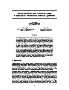
metric tensor for shape comparison, deformation tensor for morphometry [1], the diffusivity tensor [2] for diffusion MRI and many others. Therefore, there is an increasing need for developing a sound and principled approach for comparing tensor fields, and in this paper we will present one such approach. The approach taken in this paper is entirely geometrical and it is based on the fundamental idea of comparing the intrinsic shapes of the tensor fields. More precisely, suppose Ti , and Tj are P(n)-valued tensor fields defined over an image domain Ω considered as a subset in Rn , where P(n) denotes the space of symmetric positive-definite n × n matrices (Figure 1). The tensor fields can naturally be regarded as submanifolds in the product space Ω × P(n). Once we have equipped Ω × P(n) with a Riemannian metric, the geometries of Ti , and Tj are then naturally defined using the induced metrics. In other words, each tensor field is considered as a kind of high-dimensional (tensorial) image graph [5]. For a grey-scale image, its image graph is a submanifold in R3 ; however, for a tensor field, its tensorial image graph is contained in a the (nonlinear) ambient space that typically has dimension greater than three. With this particular viewpoint, comparisons between tensor fields can be formulated intrinsically as comparisons between their corresponding tensorial image graphs, and the method of [4] can be generalized directly to this higher-dimensional context by computing the registration between two shapes embedded in the ambient space.

(a)

(b)

Fig. 1. Left: The tensorial image graph of a tensor field defined on R3 . The ambient space is the cartesian product R3 × P(3). Right: Comparing shapes in R3 × P(3) can be realized via a registration map X defined between the two shapes.

The approach outlined above offers several important advantages over the relatively straightforward L2 -based approach. First, it is conceptually transparent and by comparing the shapes (instead of tensor fields) directly on the tensorial image graphs, the issue of parametrization invariance becomes irrelevant and the complicated procedures of finding a parametrically invariant representation [2] can be completely bypassed. Second, the issue of symmetric comparison and registration [3] is naturally incorporated through the use of intrinsic volume forms defined on the shapes. Third, while the mathematics is more involved when compared with the L2 -based methods, it is still tractable and we have developed a gradient descent-based method to efficiently optimize the objective function. Fi-

Matching and Classification of Images Using The Space of Image Graphs

101

nally, the proposed approach is also flexible in that it permits different metrics to define different shapes for a given tensor field. For example, the ambient space Ω × P(n) can be equipped with several different metrics (for example, the usual Frobenius metric and affine-invariant metric on P(n)), and our approach can easily accommodate these different choices. For validation, we apply the proposed method to classify brain MRI from different population groups contained in the OASIS database [10] which includes the challenging problem of classifying MR brain scans of patients suffering from the alzheimer’s disease and that of normal healthy old adults. The MR brain images are first converted into their corresponding tensor representations, and pairwise similarities between the resulting tensor fields are computed using the proposed method. Nonlinear dimensionality reduction of the data is achieved using a diffusion map [11] with the pairwise similarities as the basic affinity measures, and the final classification step is carried out efficiently and accurately in a low-dimensional Euclidean space. In terms of better and stronger classification results, the experimental results reported in section 4 validate the two novel points advocated in this paper that the tensor field comparisons are fundamental and important in many applications, and a sound and principled approach to tensor field comparison can form the basis of algorithmic solutions to challenging classification problems.

2

Cost Function for Shapes Matching

Shapes can be represented as Rn -dimensional point clouds, triangular meshes, or parametric or implicit surfaces. In this paper, shapes are considered as parametric surfaces. For instance, surfaces in 3-D are represented parameterically by : f : Ω → R3 ,where Ω is a domain. If we represent images as image graphs in order to represent images as shapes, the desired parameterization is f : (u, v) → (x, y, I(x, y)) for 2-D gray scale images or f : (u, v) → (x, y, P (3)(x, y)) for 2-D 3-by-3 symmetric positive definite (SPD) tensor-valued images. More precisely, an image can be considered as a section of a fiber bundle [5]. Then for a pair of shapes (S1 , S2 ), a matching problem can be formulated as follows :  √ (1) D((S1 , S2 ), γ) = min Dist(S1, S2 ◦ γ) κdΩ, γ

where S1 and S2 share common domain Ω. On this stage we assume that shapes are already globally registered. In Eq.(2), Dist(S1 , S2 ) is√a point-wise distance defined in the ambient space between two shapes and √κdΩ is volumef orm defined as ||dfp (u) × dfp (v)|| where f : (u, v) → p and κ is invariant under re-parametrization. For shape comparison, D((S1 , S2 ), γ) is required to be invariant under reparametrization, and symmetric between S1 and S2 . Recently, [2] introduces the notion of q − map as a novel representation for shapes in R3 with the aim of achieving re-parametrization invariance of D((S1 , S2 ), γ). However if the ambient space is not Euclidean, e.g., P(3), it is not clear how to complete the centering

102

Seo, Ho, Vemuri

step in the construction of the q − map in [2]. A similar cost function as Eq.(2) was proposed earlier in [4] which is designed for matching 3-D face meshes. However, the proposed matching algorithm is not symmetric and nor is it designed for matching tensorial image graphs. In this paper, we introduce a novel symmetric matching framework for lowdimensional shapes embedded in an ambient space X that generally has dimension greater than three. Such shapes will be represented by their parameterizations with domains in R2 or R3 . Let S1 and S2 be two such surfaces with parameterizations f1 and f2 defined on two domains Ω1 and Ω2 respectively. We will use the following cost function to define a similarity measure between these two shapes   √ E((S1 , S2 ), γ) = min (Dist(f1 , f2 ◦ γ))2 ( κ1 + κ2 (Ω2 ◦ γ)Jγ )dΩ, (2) γ

√ √ where κ1 dΩ1 and κ2 dΩ2 are the pull-backs of the volume form on S1 , S2 under f1 and f2 , respectively. Ω = Ω1 , and Jγ is the determinant of the Jacobian of γ. The details of derivation of Eq.(2) is given in the appendix. 2.1

Tensorial Image Graphs

In this section, we apply our matching framework to tensor-valued images, specifically 3-by-3 3-D SPD tensor-valued images. For this purpose, each tensor-valued image is represented as a section of a fiber bundle [5] with the map X : R3 → R3 × P(3) or X : (u, v, w) → (x(u, v, w), y(u, v, w), z(u, v, w), I(x, y, z)). In this map, x = u,y = v,z = w and I(x, y, z) ∈ P(3) at each voxel. This parametrization was introduced by Gur et. al [5] to achieve √ anisotropic smoothing of 2-D DTI. In this appplication, the volume form is κdudvdw where κ is the determinant of ⎛ ⎞ < Xu , Xu > < Xu , Xv > < Xu , Xw > K = ⎝ < Xu , Xv > < Xv , Xv > < Xv , Xw > ⎠ , (3) < Xu , Xw > < Xv , Xw > < Xw , Xw > or

⎞ λ + T r((I −1 Ix )2 ) T r((I −1 Ix )(I −1 Iy )) T r((I −1 Ix )(I −1 Iz )) K = ⎝ T r((I −1 Ix )(I −1 Iy )) λ + T r((I −1 Iy )2 ) T r((I −1 Iy )(I −1 Iz )) ⎠ , (4) T r((I −1 Ix )(I −1 Iz )) T r((I −1 Iy )(I −1 Iz )) λ + T r((I −1 Iy )2 ) ⎛

and the metric in the ambient space is given by: ⎞ ⎛ λ00 0 ⎜0 λ 0 0 ⎟ ⎟ G=⎜ ⎝0 0 λ 0 ⎠, 000P

(5)

where P is the metric in P(3) space. We will call the shapes (submanifolds) represented by the parametrization X as the tensorial image graph of the tensorvalued images I. Representing the tensorial image graphs S1 and S2 by (x1 , y1 , z1 , I1 )

Matching and Classification of Images Using The Space of Image Graphs

103

and (x2 , y2 , z2 , I2 ) respectively, we define Dist((S1 , S2 ), γ) in Eq.(2) by: Dist((S1 , S2 ), γ) = λ((x1 − x2 )2 + (y1 − y2 )2 + (z1 − z2 )2 ) + dist(I1 , I2 ), (6) and

−1/2

dist(I1 , I2 ) = T race(log(I1

−1/2 2

R† (I2 ◦ γ)RI1

) ).

(7)

Eq.(7) is voxel-wise Riemannian distance between tensors [6], with R the matrix used to re-orient the tensors (as they undergo a registration). When we choose Ω as the common domain, (x1 , y1 , z1 ) = (u, v, w) and (x2 , y2 , z2 ) = (u + U (u, v, w), v + V (u, v, w), w + W (u, v, w)), where U, V, W are the components of the deformation field. In Eq.(7), R is reoriented with respect to the deformation vector field γ (or U, V, W ) at each voxel. Reorientation of tensors must be carried out during optimization to and the reorientation transformation

is derived from the deformation field [7, 8]. Also, recall that T race((log(A)2 ) = 3i=1 (log(Λi ))2 , where Λi ’s are the eigenvalues of A. To smooth the vector field, (U, V, W ), we add the regularization term to Eq.(2) :  |∇U |2 + |∇V |2 + |∇W |2 dΩ,

Ereg =

(8)

and the final cost function, Etot ((S1 , S2 ), γ) is given as: Etot ((S1 , S2 ), γ) = (1 − α)E((S1 , S2 ), γ) + αEreg ,

(9)

where α is a small positive scalar. To efficiently solve the resulting optimization problem, we first discretize the cost function to get,  √ √ Etot (U, V, W) = [(1 − α)Dist(Ui , Vi , Wj )( κ1i + κ2i Jγi ) (10) i∈Ω

+α



2 2 (Uki + Vki2 + Wki )]

k={x,y,z}

where Ui , Vi , Wj , Uki , Vki , Wki are the values of U, V, W at the given discrete points. We optimize the above cost function with respect to U, V, W using nonlinear conjugate gradient (NCG) method following [9]. To simplify the steps, we evaluate the gradient vector and the Hessian matrix of Eq.(10) with fixed √ √ √ √ ( κ1i + κ2i Jγi ) in each NCG iteration, and in turn, ( κ1i + κ2i Jγi ) is computed using the most recently updated deformation vector field, (Ui , Vi , Wi ).

3

Application : Classification of MRI data

To apply our matching framework to classification of tensor-valued image data set, we first convert the input images into their associated tensor-valued images (tensor fields) and compute pairwise matching. In the second step, we use the L2 norms of the deformation vector fields, d(Si , Sj ) between the two tensorial

104

Seo, Ho, Vemuri

image graphs Si and Sj to build a data graph with Gaussian weights e−d(Si ,Sj )/ according to [11]. The corresponding Markov matrix is used to compute the diffusion maps [11], which provides a dimensionality reduction of the input image data. The nearest neighbor classifier is then used for classification using the diffusion distances in the low-dimensional feature space. 3.1

Data Preparation

To create 3-D tensor images from a 3D gray-scale images, we used the OASIS MRI database [10]. The images in the database are the MR human brain scans of subjects aged between 18-96 of 416. Each image has a resolution of 208×176×176 voxels. Our goal is to classify the MR image data into different age groups, and we have chosen the ventricle as the ROI (region of interest) as it captures the part of brain showing the most significant difference across ages. Fig.2 shows ROIs from sagittal and longitudinal MR slices acquired from brains of 18, 43 and 81 year old subjects respectively. Our tensor-valued images are the first fundamental forms (metric tensors) of image graphs of the 3-D intensity values with map f : R3 → R3 × R, ⎛ ⎞ < fu , fu > < fu , fv > < fu , fw > ⎝ < fu , fv > < fv , fv > < fv , fw > ⎠ , (11) < fu , fw > < fv , fw > < fw , fw > and we consider these tensor fields as tensorial image graphs. Fig.3 shows the tensor-valued images from subjects in Fig.2 according to Eq.11. 3.2

Diffusion Map and Diffusion Distance for Classification

In this paper, we represent the SPD tensor-valued images as sections of a fiber bundle, therefore we need to find a meaningful geometric description of the space of sections for classification purposes and diffusion maps can generate efficient representation of desired geometric structures based on the diffusion processes.[11] Once we build a graph with Gaussian weights e−d(Si ,Sj )/ and construct the corresponding Markov matrix, M, then the family of diffusion maps {Ψt }t∈N and diffusion distance Dt (Si , Sj ) are defined as follows : ⎞ Λt1 Ψ1 (Si ) ⎜ Λt2 Ψ2 (Si ) ⎟ ⎟ ⎜ Ψt (Si ) = ⎜ ⎟, .. ⎠ ⎝ . ⎛

(12)

Λts Ψs (Si ) and

Dt (Si , Sj ) =

s  l=1

1/2 Λ2t l (Ψl (Si )

2

− Ψl (Sj ))

,

(13)

Matching and Classification of Images Using The Space of Image Graphs

105

where {Λl }l≥0 and {Ψl }l≥0 are eigenvalues and eigenvectors of M respectively such that 1 = Λ0 > |Λ1 | ≥ |Λ2 | ≥ . . . and MΨl = Λl Ψl (Ref.), and s = max{l ∈ N such that|Λl |t > δ|Λ1 |t }.

(14)

The diffusion map Ψt embeds all data in the set, {Si } into the Euclidean space Rs and Dt reflects the connectivity in the graph of the data in the set, {Si } defining the Euclidean distance in Rs : points in the set {Si } are closer if they are highly connected in the graph.  We set d(Si , Sj ) as L2 norm of deformation vector fields, or (|U |2 + |V |2 + |W |2 )dΩ, after matching and use the diffusion distance as feature of nearest neighbor classifier in the low dimensional space. Fig.4 shows Ψ1 vs. Ψ2 plots for classifications between groups. The details of classification results are reported in next section.

4

Experimental Results

In this section, we report the experimental results on classifications of MR brain images from the OASIS data set. We divided the subjects into three groups : the young group with age below 40, the old group with age 60 or above and the middle-aged group between 41-60. In these experiments, we use a four-fold crossvalidation and leave-one-out validation to determine the classification scores. In the four-fold cross-validation, the subgroups are randomly selected 50 times and the maximum, minimum and average classification scores together with the variances are reported in the first three columns in Table 1. We also test our method to classify Alzheimer’s disease (AD). We take 70 subjects from old age group and in the subgroup, 35 of them are diagnosed as AD and rest of them are control, and we use four-fold and leave-one-out validation tests within the subgroup[13]. The classifier used in the reduced dimension is the nearestneighbor classifier, and the diffusion distance is used as distance measure. The criterion for determining the dimension of the diffusion map in these experiments is given by δ = 0.07 in Eq.(14) with t = 1. The metric used for the ambient space R3 × P(3) is the product metric of the Euclidean metric on R3 and the affineinvariant metric on P(3). Furthermore, tensor reorientation [7],[8] is applied to reorient the tensors after transformation. We note that for three different sets of classification, the classification rates are uniformly high. In the second set of experiments, we test the effects of using tensor field (compared with only scalar field) and the choice of different metric on P(3). First, we change the metric on P(3) from the affine-invariant metric to the Frobenius norm (i.e., L2 -norm), and four-fold cross-validation results between young and old age group are reported in the first two columns in Table 2. In these two columns, we test the effect of tensor reorientation on classifications, and the results show that for Frobenius norm, the effect is generally small. In the third column, the images are represented by their image graphs and the shape comparisons are carried out in the ambient space R3 × R instead of R3 × P(3). In this experiment, distances between image graphs are the Riemannian distances

106

Seo, Ho, Vemuri

and λ = 0.000001 in Eq.(6) and α = 0.02 in Eq.(9). We remark that the result clearly demonstrates that the classification result using only scalar-valued images (image graphs in R3 ) is inferior to the one using tensor fields and the affineinvariant metric on P(3) provide superior classification result compared with the Frobenius metric. In Table 3, we show the comparisons between our method and several previously published classification results on the OASIS database. [12] uses the deformation tensor field (computed from registering the image to an atlas) as the main feature for each image. Submanifold of each age group is constructed from the training samples and the geodesic distances between subjects and the submanifolds are used as the main discriminative feature for classification. In [13], alternatively, histograms of deformation vector fields have been used as features, and the CAVIAR method proposed in [13] takes a adaboost-like approach to integrate the results from a collection of weak classifiers into a strong classification result. We remark that our method compared favorably with these methods in terms of classification rates, and in particular, for the more challenging problem of classifying brain images of Alzheimer’s disease patients, our method demonstrates a small but real improvement over these two methods. Table 1. Scores of leave-one-out and four-fold cross-validation test of four subgroups randomly selected 50 times. The metric used for the ambient space R3 × P(3) is the product metric of the Euclidean metric on R3 and the affine-invariant metric on P(3).

Maximum Minimum Average Standard deviation Leave-one-out

Old vs. Young Old vs. Middle Middle vs. Young AD vs. Control 100% 100% 100% 100% 97.72% 90.77% 87.27% 75.0% 99.25 % 97.6% 94.36 % 94.87% 0.8384% 2.46% 3.09% 5.55% 99.15 % 98.46 % 96.36% 95.32%

Table 2. Scores of leave-one-out and four-fold cross-validation test of four subgroups randomly selected 50 times between Young and Old samples using Frobenius metric on P(3) with and without tensor re-orientation. Last column gives the classification result of using only gray-scale images. Methods Frobenius with reo. Frobenius without reo. Image Graph Maximum 100% 100% 98.86% Minimum 88% 88.63% 88.63% Average 94.96 % 96.52% 94.29 % Standard deviation 2.57% 2.15% 2.29% Leave-one-out validation 97.03% 98.01% 94.89%

Matching and Classification of Images Using The Space of Image Graphs

107

Table 3. Comparison of classification scores with 4-fold validation between classification methods Image Graphs CAVIAR [13] Adaboost [13] Submanifold projection [12] Nearest Neighbor in PCA [12]

5

Old vs. Young Old vs. Middle Middle vs. Young AD vs. Control 99.25% 97.6% 94.36% 94.87% 99.14 % 98.36 % 97.76% 88.0% 98.75 % 96.80 % 96.0% 90.25 % 96.43% 90.23% 84.32% 88.57% 92.43% 87.74 % 78.42 % 84.29 %

Conclusion

We have proposed a novel geometric approach for comparing tensor-valued images (tensor fields) that is based on the simple idea of matching the low-dimensional tensorial image graphs formed by the tensor fields. Our framework provides a registration method that is both symmetric and invariant under different parametrization, and the resulting cost function can be satisfactorily optimized using a gradient descent-based method. We have reported four different classification experiments using the OASIS image database, and our method has produced results that are in par or exceeding the current state-of-the-art results. In particular, our experiments have shown that tensor fields do indeed contain subtle information that can be useful for challenging classification problems, and the experimental results have demonstrated that the proposed method, although more elaborat and involved compared with L2 -based method, is able to access and utilize this information to obtain good classification results.

References 1. N. Lepore, C. Brun, Y. Chou, M. Chiang, R. A. Dutton, K. M. Hayashi, E. Luders, O. L. Lopez, H. J. Aizenstein, A. W. Toga, J. T. Becker, P. M. Thompson, “Generalized Tensor-Based Morphometry of HIV/AIDS Using Multicariate Statistics on Deformation Tensors”, IEEE Transations on Medical Imaging, 2008. 2. S. Kurtek, E. Klassen, Z. Ding and A. Srivastava, “A novel riemannian framework for shape analysis of 3D objects”, Proc. CVPR pp. 1625-1632, 2010. 3. H. D. Tagare, D. Groisser and O. Skrinjar, “Symmetric Non-rigid Registration : A Geometric Theory an Some Numerical Techniques” , J Math Imaging Vis pp. 61-88, 2009. 4. N. Litke, M. Droske, M. Rumpf and P. Schr¨ oder, “An Image Processing Approach to Surface Matching”, in “Symposium on Geometry Processing”, pp. 207-216, 2005. 5. Y. Gur and N. Sochen, “Coordinate-based diffusion over the space of symmetric positive-definite matrices”, in “Visualization and Processing of Tensor FIelds - Advances and Perspectives”, pp 325-340, Springer-Verlag, Berlin Heidelberg, 2009 . 6. M. Moakher and P. G. Batchelor, “Symmetric Positive-Definite Matrices: From Geometry to Applications and Visualization”, in “Visualization and Processing of Tensor FIelds”, pp285-298 , Springer-Verlag, New York, 2006.

108

Seo, Ho, Vemuri

7. G. Cheng, B. C. Vemuri, M. Parekh, P. R. Carney, and T. H. Mareci, “Non-rigid Registration of HARDI Data Represented by a Field of Gaussian Mixtures”, In LNCS (Springer) Proceedings of MICCAI09: Int. Conf. on Medical Image Computing and Computer Assisted Intervention, 2009. 8. D. C. Alexander, C. Pierpaoli, P. J. Basser, and J. C. Gee, “Spatial Transformations of diffusion tensor magnetic resonance images”, IEEE Trans. Med. Imag. 20 11 pp. 1131-1139, 2001. 9. S.H. Lai and B. C. Vemuri, “Reliable and Efficient Computation of Optical Flow”, IJCV 29(2), pp. 87-105, 1998. 10. D. S. Marcus, T. H. Wang, J. parker, J. G. Csernansky, J. C. Moris, R. L. Buckner “Open Access Series of Imaging Studies (OASIS): Cross-Sectional MRI Data in Young, Middle Aged, Nondemented, and Demented Older Adults”. Journal of Cognitive Neuroscience (2007) 11. R. R. Coifman and S. Lafon, “Diffusion Maps”, Appl. Comput. Harmon. Anal. 21 pp. 5-30, 2006 12. Y. Xie, B. C. Vemuri, and J. Ho, “Statistical Analysis of Tensor Fields ”, In Int. Conf. on Medical Image Computing and Computer Assisted Intervention (MICCAI), 2010. 13. T. Chen, A. Rangarajan, and B. C. Vemuri, “CAVIAR: Classification via Aggregated Regression and Its Application in Classifying the OASIS Brain Database”, In IEEE International Symposium on Biomedical Imaging, pp. 1337-1340, 2010.

Appendix. Cost Function for Symmetric Matching If we have two parameterized shapes, S1 and S2 with domain Ω1 and Ω2 , then the cost function for symmetric matching problem is formulated as following :   √ √ E((S1 , S2 ), φ, ψ) = min Dist(S1 , S2 ◦φ) κ1 dΩ1 +min Dist(S2 , S1 ◦ψ) κ2 dΩ2 , φ

ψ

Ω1

Ω2

(A-1) √ where φ : Ω1 → Ω2 and ψ : Ω2 → Ω1 , and κdΩ is volumef orm. If The second term in the left hand side of Eq(A-1) can be rewritten as following :   Dist(S2 ◦ ψ −1 , S1 ) κ2 (Ω2 ◦ ψ −1 )Jψ−1 dΩ1 , (A-2) Ω1

and if we require that Eq(A-1) is symmetric matching, ψ −1 should be φ and Jψ−1 = Jφ which is determinant of Jacobian such as ⎛ ⎞ ⎜ Det ⎝

∂u2 ∂u1 ∂v2 ∂u1 ∂w2 ∂u1

∂u2 ∂v1 ∂v2 ∂v1 ∂w2 ∂v1

∂u2 ∂w1 ∂v2 ∂w1 ∂w2 ∂w1

⎟ ⎠

And κ2 is determinant of K2 given as following : ⎛ ⎞ < S2 u2 , S2 u2 > < S2 u2 , S2 v2 > < S2 u2 , S2 w2 > K2 = ⎝ < S2u2 , S2v2 > < S2v2 , S2v2 > < S2v2 , S2w2 > ⎠ < S2 u2 , S2 w2 > < S2 v2 , S2 w2 > < S2 w2 , S2 w2 > 

= (Jφ−1 )2 K2 ,

(A-3)

(A-4) (A-5)

Matching and Classification of Images Using The Space of Image Graphs

and

109

⎛

⎞ < S2u1 , S2u1 > < S2u1 , S2v1 > < S2u1 , S2w1 > K2 = ⎝ < S2 u1 , S2 v1 > < S2 v1 , S2 v1 > < S2 v1 , S2 w1 > ⎠ < S2 u1 , S2 w1 > < S2 v1 , S2 w1 > < S2 w1 , S2 w1 > 

(A-6)

Finally the cost function is given as following :   √  Dist(S1 , S2 ◦ φ)( κ1 + κ2 )dΩ1 , E((S1 , S2 ), φ, ψ) = min φ



(A-7)

Ω1



where κ2 is the determinant of K2 .

(a)

(b)

(c)

(d)

(e)

(f)

Fig. 2. Slices of 3-D MRI images. (a)-(c) : Cross-sectional images of ventricles of 18, 43, and 81 years old respectively. (d)-(f): Longitudinal images of ventricles in the same order.

110

Seo, Ho, Vemuri

(a)

(b)

(c)

Fig. 3. Slices of 3-D tensor images of ventricles created by Eq.(11). (a)-(c) : 18, 43, and 81 years old respectively. Young vs Old

Young vs Middle

0.15

0.3 Young Old

Young Middle 0.2

0.05

0.1

0

0

Ψ

2

Ψ2

0.1

−0.05

−0.1

−0.1

−0.2

−0.15

−0.3

−0.2 −0.15

−0.1

−0.05

Ψ1

0

0.05

−0.4 −0.15

0.1

−0.1

−0.05

0

(a)

0.05

Ψ1

0.1

0.15

0.2

0.25

0.3

(b) Middle vs Old 0.15 Middle Old 0.1

0.05

Ψ2

0

−0.05

−0.1

−0.15

−0.2

−0.25 −0.2

−0.15

−0.1

−0.05

Ψ

0

0.05

0.1

0.15

1

(c) Fig. 4. 2-D plots of diffusion maps: (a) young vs. old, (b) young vs. middle, and (c) middle vs. old. In each plot, x-axis and y-axis are Ψ1 and Ψ2 , respectively