IEEE TRANSACTIONS ON GEOSCIENCE AND REMOTE SENSING, VOL. 41, NO. 3, MARCH 2003
675
Unsupervised Classification of Radar Images Using Hidden Markov Chains and Hidden Markov Random Fields Roger Fjørtoft, Member, IEEE, Yves Delignon, Member, IEEE, Wojciech Pieczynski, Marc Sigelle, Member, IEEE, and Florence Tupin
Abstract—Due to the enormous quantity of radar images acquired by satellites and through shuttle missions, there is an evident need for efficient automatic analysis tools. This paper describes unsupervised classification of radar images in the framework of hidden Markov models and generalized mixture estimation. Hidden Markov chain models, applied to a Hilbert–Peano scan of the image, constitute a fast and robust alternative to hidden Markov random field models for spatial regularization of image analysis problems, even though the latter provide a finer and more intuitive modeling of spatial relationships. We here compare the two approaches and show that they can be combined in a way that conserves their respective advantages. We also describe how the distribution families and parameters of classes with constant or textured radar reflectivity can be determined through generalized mixture estimation. Sample results obtained on real and simulated radar images are presented. Index Terms—Generalized mixture estimation, hidden Markov chains, hidden Markov random fields, radar images, unsupervised classification.
I. INTRODUCTION
B
OTH visual interpretation and automatic analysis of data from imaging radars are complicated by a fading effect called speckle, which manifests itself as a strong granularity in detected images (amplitude or intensity). For example, simple classification methods based on thresholding of gray levels are generally inefficient when applied to speckled images, due to the high degree of overlap between the distributions of the different classes. Speckle is caused by the constructive and destructive interference between waves returned from elementary scatterers within each resolution cell. It is generally modeled as a multiplicative random noise [1], [2]. At full resolution (single-look images), the standard deviation of the intensity is
Manuscript received December 4, 2001; revised October 3, 2002. This work was supported by the Groupe des Ecoles des Télécommunications (GET) in the framework of the project “Segmentation d’images radar.” R. Fjørtoft is with the Norwegian Computing Center (NR), 0314 Oslo, Norway (e-mail:
[email protected]). Y. Delignon is with the Ecole Nouvelle d’Ingénieurs en Communications (ENIC), Département Electronique, 59658 Villeneuve d’Ascq, France (e-mail:
[email protected]). W. Pieczynski is with the Institut National des Télécommunications, Département CITI, 91011 Evry, France (e-mail:
[email protected]). M. Sigelle and F. Tupin are with the Ecole Nationale Superieure des Télécommunications, Département TSI, 75634 Paris, France (e-mail:
[email protected];
[email protected]). Digital Object Identifier 10.1109/TGRS.2003.809940
equal to the local mean reflectivity, corresponding to an SNR of 0 dB. One possible way to overcome this problem is to exploit spatial dependencies among different random variables via a hidden Markov model. Markov random fields are frequently used to model stochastic interactions among classes and to allow a global Bayesian optimization of the classification result [3], according to criteria such as the maximum a posteriori (MAP) or the maximum posterior marginal (MPM) [3]–[10]. However, the computing time is considerable and often prohibitive with this approach. A substantially quicker alternative is to use Markov chains, which can be adapted to two-dimensional (2-D) analysis through a Hilbert–Peano scan of the image [11]–[14]. In the case of unsupervised classification, the statistical properties of the different classes are unknown and must be estimated. For each of the Markov models cited above, we can estimate characteristic parameters with iterative methods such as expectation–maximization (EM) [15]–[17], stochastic expectation–maximization (SEM) [18], or iterative conditional estimation (ICE) [19], [20]. Classic mixture estimation consists in identifying the parameters of a set of Gaussian distributions corresponding to the different classes of the image. The weighted sum (or mixture) of the distributions of the different classes should approach the overall distribution of the image. In generalized mixture estimation, we are not limited to Gaussian distributions, but to a finite set of distribution families [14], [21]. For each class we thus seek both the distribution family and the parameters that best describe its samples. In this paper, we consider some distribution families that are well adapted to single- or multilook amplitude radar images and to classes with or without texture [2]. By texture, we here refer to spatial variations in the underlying radar reflectivity and not the variations due to speckle. According to the multiplicative noise model, the observed intensity is the product of the radar reflectivity and the speckle. In this study, we limit ourselves to the ICE estimation method and the MPM classification criterion. When analyzing an image, the only input parameters entered by the user is the number of classes and the list of distribution families that are allowed in the generalized mixture. The estimation and classification schemes are described separately for the two Markov models. We compare their performances and show in particular that the Markov chain method can compete with the Markov random field method in terms of estimation and classification accuracy, while being much faster. We furthermore introduce a hybrid
0196-2892/03$17.00 © 2003 IEEE
676
IEEE TRANSACTIONS ON GEOSCIENCE AND REMOTE SENSING, VOL. 41, NO. 3, MARCH 2003
method that combines the speed and robustness of the estimation and classification methods based on Markov chains with the fine spatial modeling of Markov random fields. Tests have been conducted on both real and simulated synthetic aperture radar (SAR) data, with different compositions of distribution families. The paper is organized as follows. In Section II, we introduce the hidden Markov random field and hidden Markov chain models, as well as the different probabilities that are needed for parameter estimation and classification. For simplicity, we first describe MPM classification in Section III, assuming known parameters for both Markov models. The ICE parameter estimation methods are presented in Section IV, first in the framework of classic mixture estimation (only Gaussian distributions) and then for generalized mixture estimation (several possible distribution families). Specific adaptations to radar images are mentioned. All the algorithms are described in sufficient detail to be implemented by readers that are familiar with statistical image processing. Estimation and classification results obtained on real and simulated SAR images with the two approaches are reported in Section V. We here also describe the improvements obtained by combining Markov chain methods and Markov random field methods in the estimation phase. Our conclusions are given in Section VI. II. MODELS Let be a finite set corresponding to the pixels of an and image. We consider two random processes . represents the observed image and the untakes its values known class image. Each random variable , whereas each from the finite set of classes takes its values in the set of real numbers. We denote realand , respecizations of and by tively.1 We here suppose that the random variables are conditionally independent with respect to and that the districonditional on is equal to its distribution bution of each .2 In practical applications, the assumption conditional on of conditional independence is often difficult to justify. However, numerous algorithms based on hidden Markov models that make this assumption have been successfully applied to real images. conditional on are then All the distributions of distributions of with respect to determined by the , which will be denoted :
Fig. 1. Pixel neighborhood and associated clique families case of four-connectivity.
C
and
C
in the
As indicated above, we will model the interactions among the by considering that the prior distrirandom variables bution of can be modeled by a Markov process. We refer to is not directly observable. it as a hidden Markov model, as from The classification problem consists in estimating . the observation A. Hidden Markov Random Fields Let denote a neighborhood of the pixel whose geometric . is a Markov random field if shape is independent of and only if
(2) i.e., if the probability that the pixel belongs to a certain class conditional on the classes attributed to the pixels in the rest of the image is equal to the probability of conditional on the classes of the pixels in the neighborhood . Assuming that the probability of all possible realizations of is strictly positive, the Hammersley–Clifford theorem [4] establishes the equivalence between a Markov random field, defined with respect to a neighborhood structure , and a Gibbs field whose potentials are associated with . The elementary relationships within the neighborhood are given by the system of cliques . Fig. 1 shows the neighborhood and the associated cliques in the case of four-connectivity. For a Gibbs field (3) is the energy of , and is a normalizing factor. The latter is in practice impossible to compute due to the very . The Hammerhigh number of possible configurations sley–Clifford theorem makes it possible to relate local and global probabilities [7], [21]. Indeed, the local conditional probabilities can be written as
where
(1) 1As
Y=y
a practical example, consider a radar image covering an area composed of agricultural fields. We can imagine a corresponding class image , where the different crops are identified by discrete labels. Each observed pixel amplitude depends on several factors, including the characteristic mean radar reflectivity and texture of the underlying class, the speckle phenomenon, the transfer function of the imaging system, and thermal noise. The latter is in general negligible. 2In the case of radar images, this means that we suppose uncorrelated speckle, i.e., that the radar system has constant transfer function. This is generally not the case, but it is often used as an approximation.
X=x
(4) is the local energy function, and is a normalizing factor. There are several ways of defining the local energy , and finding a good compromise between its modeling power—which increases when its complexity increases—and the possibilities for efficient estimation of it in unsupervised classification methods—which decreases when its complexity increases—remains an open problem. For simplicity, we will
where
FJØRTOFT et al.: UNSUPERVISED CLASSIFICATION OF RADAR IMAGES
677
restrict ourselves to Potts model, four-connectivity and cliques [7], in which case is the number of of type for which , minus the number of pixels pixels for which , multiplied by a regularity parameter . The global energy in (3) is computed in a similar way, except that we sum the potentials over all vertical and horizontal cliques in the image. As will be explained later, it can be and advantageous to have different regularity parameters horizontally and vertically. Bayes’ rule and the conditional independence of the samples (1) allow us to write the a posteriori probability as
(a)
(b)
Fig. 2. Construction of a Hilbert–Peano scan for an 8 Initialization. (b) Intermediate stage. (c) Result.
. According to the definition,
(c)
2
8 image. (a)
is a Markov
chain if
(7) (5)
. The distribution of will consequently be for , denoted by , and the set determined by the distribution of , whose elements are of transition matrices . We will in the following assume that the probabilities
(6)
(8)
and the corresponding local conditional distributions as
are independent of . The initial distribution then becomes and are normalizing factors obtained by summing where over all possible nominators, similar to and . Substituting into (5), we see that conditional on is a Gibbs field (3). It is not possible to create a posteriori realizations of according to (5) directly, but they can be approximated iteratively with the Metropolis algorithm [22] or Gibbs sampler [5]. We will here only consider Gibbs sampler, which includes the following steps. • We start from an initial class image . • We sweep the image repeatedly until convergence. For each iteration and for each pixel a) the local a posteriori distribution given by (6) is computed; b) the pixel is attributed to a class drawn randomly according to this distribution.3 In a similar way, a priori realizations of obeying (3) can be computed iteratively using (4). B. Hidden Markov Chains A 2-D image can easily be transformed into a one-dimensional chain, e.g., by sweeping the image line by line or column by column. Another alternative is to use a Hilbert–Peano scan [11], as illustrated in Fig. 2. Generalized Hilbert–Peano scans [12] can be applied to images whose length and width are not powers of two. In a slightly different sense than above, now let and be the vectors of random variables ordered according to such a transformation of the class image and the observed image, respectively. Their reand alizations will consequently be denoted
(9) and the transition matrix given by
is constant (independent of ) and (10)
is that of a stationary Hence, the a priori distribution of parameters Markov chain. It is entirely determined by the , and we can write
(11) where is the index of the class of the th element of the chain. The so-called forward and backward probabilities (12) and (13) can be calculated recursively. Unfortunately, the original forward–backward recursions derived from (12) and (13) are subject to serious numerical problems [13], [23]. Devijver et al. [23] have proposed to replace the joint probabilities by a posteriori probabilities, in which case (14) and
3Random
sampling of a class according to a distribution can be done in the following way: We consider the interval [0,1] and attribute to each class a subinterval whose width is equal to the probability of that class. A uniformly distributed random number in [0,1] is generated, and the class is selected according to the subinterval in which this random number falls.
(15)
678
IEEE TRANSACTIONS ON GEOSCIENCE AND REMOTE SENSING, VOL. 41, NO. 3, MARCH 2003
In the following, we use the numerically stable forward–backward recursions resulting from these approximations: • Forward initialization
and is obtained by random sampling according to this distribution. III. CLASSIFICATION
(16) . for • Forward induction (17) and for • Backward initialization
. (18)
. for • Backward induction (19) and . for The joint probability of the classes of two subsequent elements given all the observations (20) can be written as a function of the forward–backward probabilities
(21) The marginal a posteriori probability, i.e., the probability of having class in element number given all the observations , can then be obtained from (21):
(22) It can be shown [14] that the a posteriori distribution of , , is that of a nonstationary Markov chain, i.e., with transition matrices given by
Let us first assume that we know the distribution and the of each class (in the case of a associated parameter vector where scalar Gaussian distribution, for example, is the mean value and the variance), as well as the regularity parameters of the underlying Markov model ( or ). In a Bayesian framework, the goal of the classification is to deterthat best explains the observation mine the realization , in the sense that it minimizes a certain cost function. Several cost functions can be envisaged, leading to different estimators, such as the MAP, which aims at maximizing the global , and the MPM, which consists a posteriori probability for in maximizing the posterior marginal distribution each pixel, i.e., finding the mode of each local posterior distribution. In this study, we use MPM classification. A. Hidden Markov Random Fields In the case of hidden Markov random fields, the MPM is computed as follows [6]. are computed • A series of a posteriori realizations of iteratively, using Gibbs sampler (or the Metropolis algorithm) based on the local a posteriori probability function (6). Each realization is obtained by generating an initial class image with a random generator and by performing a certain number of iterations with Gibbs sampler (until approximate convergence of the global energy ). • For each pixel , we retain the most frequently occurring . class The required number of a posteriori realizations and iterations per realization will be discussed in Section V. B. Hidden Markov Chains The MPM solution can be calculated directly for hidden Markov chains, based on one forward–backward computation. • For every element in the chain, and for every possible class , we compute (17); a) forward probabilities (19); b) backward probabilities (22). c) marginal a posteriori probabilities that maxi• Each element is attributed to the class mizes . IV. MIXTURE ESTIMATION
(23) Using (23), we can simulate a posteriori realizations of directly, i.e., without iterative procedures as in the case of hidden of the first element of Markov random fields. The class the chain is drawn randomly according to the marginal a poste(22). Subsequently, for each new element riori distribution , the transition probabilities (23) are combeing fixed, puted, the class of the precedent element
In practice, the regularity parameters and the parameters of the distributions of the classes are often unknown and must be . As the distribution of estimated from the observation can be written as a weighted mixture of probability densi, such a problem is called ties, a mixture estimation problem. The problem is then double: we do not know the characteristics of the classes, and we do not know which pixels are representative for each class. We first present classic mixture estimation, where all classes are supposed to be Gaussian, and then introduce generalized mixture
FJØRTOFT et al.: UNSUPERVISED CLASSIFICATION OF RADAR IMAGES
679
estimation, where several distribution families are possible for each class. There are several iterative methods for mixture estimation, including EM [15], SEM [18], and ICE [19], [20]. Here we will only consider ICE, which has some relations with EM [24]. The ICE method has been applied to a variety of image analysis problems, including classification of forest based on remote sensing images [25], segmentation of sonar images [26], segmentation of brain SPECT images [27], video segmentation [28], multiresolution image segmentation [29], and fuzzy image segmentation [30], [31]. In this paper, we also use the generalized ICE, which is an extension of the classic ICE to the case where the distribution family can vary with the class and is not known. We will only present what is necessary for the implementation, and not the underlying theory, which can be found in [14] for hidden Markov chains, and in [21] for hidden Markov random fields. Furthermore, we propose a special version of the ICE for hidden Markov random fields, where the estimation of the regularity parameter is inspired by the generalized EM method proposed in [32]. A. Hidden Markov Random Fields The ICE algorithm iteratively creates a posteriori realizations and recalculates the class and regularity parameters. In the framework of classic mixture estimation, the following computation steps are carried out for each iteration . • A certain number of a posteriori realizations (with index ) are computed with Gibbs sampler, using the parameters (defining ) obtained in the previous iteration. are estimated for each a poste• The class parameters . riori realization and then averaged to obtain • The regularity parameter is estimated with a stochastic gradient approach [32]–[35], based on a series of a priori realizations computed with Gibbs sampler. Gibbs sampler is initialized with a random image for each a priori or a posteriori realization. In order to reduce the computation time, we generally compute only one a posteriori realization for each iteration of the ICE and only one a priori realization for each iteration of the stochastic gradient. This simplification does not imply any significant performance loss. We use a coarse approximation of the stochastic gradient be the energy (3) of equation to compute . Let the energy of the current a posteriori realization and the a priori realization in iteration of the stochastic gradient. to , i.e., the value obtained in the precedent Setting compute until ICE iteration, we repeatedly convergence
attributed samples at the end of each iteration. It should be noted that this method only can be used to initiate classes with different mean values. It is, for example, not suited when classes with the same mean value but different variance must be distinguished. K-means is basically a thresholding method, so if there is much overlap between the true class distributions, as for radar images, the resulting class image will be quite irregular and the initial class statistics will not be very representative. The consequences of this, and a possible remedy, will be commented on in Section V. The initial value of is predefined (typically ). B. Hidden Markov Chains We initiate the ICE algorithm in a similar way for hidden Markov chains, using K-means to define the class parameand thus the marginal conditional distributions , ters uniformly distributed a priori probabilities , and a generic where when and transition matrix when . Each ICE iteration is based on one forward–backward computation and includes the following steps. • For every element in the chain, and for every possible class , we compute (17) based on , a) forward probabilities , and (given by ); (19) based on , b) backward probabilities , and ; (22). c) marginal a posteriori probabilities • This allows us to compute (21) a) new joint conditional probabilities , , , and ; using b) new elements of the stationary transition matrix (25) c) new initial probabilities (26)
• We compute a series of a posteriori realizations based on , , and . For each realization (with (23) with , which are index ), we estimate the class parameters and thus . averaged to obtain As for hidden Markov random fields, we generally limit the number of a posteriori realizations per ICE iteration to one.
(24) C. Generalized Mixture Estimation The ICE algorithm needs an initial class image from which the initial parameters of the classes are computed. We have used the K-means algorithm, which subdivides the gray levels in K distinct classes iteratively. The initial class centers are uniformly distributed over the range of gray levels. We sweep the image repeatedly until stability, attributing each pixel to the class with the closest center, and recompute the class centers from all the
In generalized mixture estimation, the distribution of each class is not necessarily Gaussian, but can belong to any distribution family in a predefined set. This implies the following modifications to the above ICE algorithms. of all possible distribution fam• The parameter vectors ilies are computed from the a posteriori realizations for each class.
680
IEEE TRANSACTIONS ON GEOSCIENCE AND REMOTE SENSING, VOL. 41, NO. 3, MARCH 2003
• The Kolmogorov distance [36] is used to determine the most appropriate distribution family for each class [14]. a) We compute the cumulative distributions for all the distribution families, based on the estimated parameters of the class. b) The cumulative normalized histogram of the class is computed. c) We retain the distribution family having the smallest maximum difference between the cumulative distribution and the cumulative normalized histogram of the class. As the pixel values are discrete, the computation and comparison of cumulative distributions and cumulative normalized histograms are straightforward. D. Application to Radar Images For simplicity, we here consider only two distribution families, corresponding to classes with constant and textured radar reflectivity, respectively. Assuming the speckle to be spatially uncorrelated, the observed intensity in a zone of constant reflectivity is Gamma distributed. The corresponding amplitude distribution is
(27) and for . . is here the for equivalent number of independent looks of the image, which should be provided by the data supplier. Let the estimated mo. Assuming that the zone of ments of order be denoted by constant reflectivity mentioned above corresponds to a certain in (27) is class, the estimated mean radar reflectivity computed over all pixels attributed to this class. If we assume that the radar reflectivity texture of a class is Gamma distributed, the observed intensity will obey a K distribution [37]–[39]. The corresponding amplitude distribution is
(28) and for . . is for here the modified Bessel function of the second kind, and the estimated radiometric parameters and are computed as foland lows. Let . If , is obtained by solving the . Otherwise equation we set , provided that . In both cases . If and , we consider (28) as unsuited, and we make sure that it is not selected. Moreover, if ), we the radar reflectivity texture is very weak (typically approximate (28) by (27). For simplicity, we will in the following refer to (27) and (28) as Gamma and K distributions, respectively, even though they actually are the amplitude distributions corresponding to Gamma and K distributed intensities. A more comprehensive set of distribution families are described in [40].
V. RESULTS The schemes for unsupervised classification of radar images described above have been tested on a wide range of real SAR images, as well as on a few simulated ones. We will here only present a small but representative selection of results. A. Real SAR Image With Three Classes Fig. 3(a) shows an 512 512 extract of a Japanese Earth Resources Satellite (JERS) three-look amplitude image of a tropical forest with some burnt plots related to agricultural activity. . It was The equivalent number of independent looks decided to classify the image into three classes. Fig. 3(b) shows the initial classification obtained with the K-means algorithm. The classes are represented by different gray levels (the gray levels do not correspond to the mean amplitudes of the different classes, but they are ordered according to these mean values). We note that the K-means class image is very irregular due to the speckle. A more regular initial classification could be obtained by applying an adaptive speckle filter prior to the K-means algorithm [41]–[43]. The subsequent mixture estimation and classification are of course carried out on the original radar image. Our tests indicate that such speckle filtering prior to the K-means initialization generally has little influence on the final classification result. Let us first consider the ICE and MPM algorithms based on the hidden Markov random fields model. We use 30 iterations for the ICE algorithm, with only one a posteriori realization per . iteration. The initial value of the regularity parameter is Within each ICE iteration, the maximum number of iterations for the stochastic gradient is set to ten, with one a priori realization per iteration. We interrupt the iteration earlier if differs less than 0.01 from its previous value. Except for the first ICE iterations, the stochastic gradient estimation generally requires very few iterations. Gibbs sampler with as much as 100 iterations is used to generate each a priori and a posteriori realization. The convergence of the global energy is in fact quite slow, especially for realizations according to the a priori distribution. The MPM classification based on the hidden Markov random fields model relies on ten a posteriori realizations. Fig. 3(c) presents the obtained classification result. The regularity param, and the Gamma eter was in this case estimated to distribution was retained for all three classes. The classification result corresponds quite well to our thematic conception of the image based on visual inspection, except that many fine structures seems to be lost, and the region borders are somewhat rounded. The number of ICE iterations is set to 30 also for the corresponding analysis scheme based on Markov chains, and we compute only one a posteriori realization per iteration. Fig. 3(d) shows the result of the MPM classification. It is generally less regular than the classification in Fig. 3(c), but it represents small structures more precisely. The K distribution was here selected by the algorithm for the darkest class, whereas the Gamma distribution gave the best fit for the two others. The overall quality is comparable for the two classification results, but the computing time is quite different: The program based on Markov random fields spent about 53 min on a
FJØRTOFT et al.: UNSUPERVISED CLASSIFICATION OF RADAR IMAGES
681
(a)
(b)
(c)
(d)
2
Fig. 3. Classification of a 512 512 extract of a JERS three-look image of a tropical forest into three classes. (a) Original amplitude image. (b) Initial K-means classification. Result obtained (c) with the Markov random field method and (d) with the Markov chain method.
PC with a Pentium III 733-MHz processor running Linux, whereas the program based on Markov chains only needed 2 min and 27 s. B. Simulated SAR Image With Three Classes In order to examine the performances more carefully, let us also consider simulated SAR images. Fig. 4(a) and (b) represents an ideal class image with three classes and its speckled counterpart. The darkest and three-look brightest classes are both Gamma distributed, whereas the one in the middle is K distributed with texture parameter (28). The contrast between two consecutive classes is 3.5 dB. The image size is 512 512 pixels. The ideal class image is in fact derived from a resampled optical image by K-means classification, so it is neither a realization of a Markov random field nor a realization of a Markov chain, but represents a natural scene. It should therefore permit a fair comparison of the two analysis schemes. The parameter settings described in Section V-A were applied here as well, except that we allowed different regularity parameters vertically and horizontally for the method based on Markov random fields, as the resolution is not the same in the two directions. The regularity parameters were estimated and , respectively. However, the to
classification result in Fig. 4(c) is far too irregular, and only 72.7% of the pixels are correctly classified. The method based on Markov chains here gives a more satisfactory result, shown in Fig. 4(d), with 83.9% of correctly classified pixels. In particular, the overall regularity of the image seems to be better estimated. Both methods correctly identify Gamma distributions for the darkest and brightest classes, but only the Markov chain method found that the class in the middle was K distributed. The fit between the estimated and the true distributions in Fig. 5 is generally very good, except for the case where the Markov random field method chooses the wrong distribution family. This can be part of the reason why the estimation of the regularity parameters here fails, but the main reason is probably the simplicity of the Markov random field model compared to the true characteristics of the ideal class image. The program based on Markov chains was here 37 times quicker than the one based on Markov random fields. C. Simulated SAR Image With Four Classes Fig. 6(a) represents an ideal and approximately isotropic 512 512 class image with four classes, which has been derived from an optical satellite image by K-means classification. Fig. 6(b) shows the corresponding simulated SAR image. The
682
IEEE TRANSACTIONS ON GEOSCIENCE AND REMOTE SENSING, VOL. 41, NO. 3, MARCH 2003
(a)
(b)
(c)
(d)
2
Fig. 4. Classification of a 512 512 simulated three-look SAR image into three classes (a) Ideal class image. (b) Speckled amplitude image. Results obtained (c) with the Markov random field method and (d) with the Markov chain method. The fraction of correctly classified pixels is (c) 72.7% and (d) 83.9%.
(a)
(b)
Fig. 5. Fit of the generalized mixture estimation performed (a) by the Markov random field method and (b) by the Markov chain method on the simulated three-look SAR image with three classes.
parameter settings and the radiometric characteristics of the classes are the same as for the simulated image with three classes shown in Fig. 4(b), except that an additional Gamma distributed
class with higher reflectivity has been added. Fig. 6(c) and (d) represents the results obtained with the Markov random field and Markov chain methods, respectively.
FJØRTOFT et al.: UNSUPERVISED CLASSIFICATION OF RADAR IMAGES
683
(a)
(b)
(c)
(d)
2
Fig. 6. Classification of a 512 512 simulated three-look SAR image into four classes. (a) Ideal class image. (b) Speckled amplitude image. Results obtained (c) with the Markov random field method and (d) with the Markov chain method. The fraction of correctly classified pixels is (c) 87.0% and (d) 85.2%.
(a)
(b)
Fig. 7. Fit of the generalized mixture estimation performed (a) by the Markov random field method and (b) by the Markov chain method on the simulated three-look SAR image with four classes.
The estimated regularity parameter for the method based on , which visually gives Markov random fields is here a very satisfactory result. The proportion of correctly classified
pixels is 87.0%, whereas it is 85.2% for the method based on Markov chains. The borders are slightly more irregular for the latter method, but some of the narrow structures are better pre-
684
IEEE TRANSACTIONS ON GEOSCIENCE AND REMOTE SENSING, VOL. 41, NO. 3, MARCH 2003
(a)
(b)
Fig. 8. Classification results for the simulated three-look SAR images with (a) three classes and (b) four classes, obtained with the new method combining Markov chain and Markov random field algorithms. The fraction of correctly classified pixels is (a) 85.8% and (b) 87.0%.
(a)
(b)
Fig. 9. Fit of the generalized mixture estimation for the simulated three-look SAR images with (a) three classes and (b) four classes, obtained with the new method combining Markov chain and Markov random field algorithms.
served. The distribution families of the four classes were correctly identified by both methods, and the fit of the estimated parameters is comparable, as can be seen from Fig. 7. The Markov chain algorithm was, however, 25 times faster. D. Hybrid Method The scheme based on Markov random fields occurs to have difficulties in estimating the regularity parameters for many images, whereas the estimation method based on Markov chains is very robust. The latter method is also much faster. Nevertheless, in cases where the Markov random field method estimates the regularity parameters correctly, it provides a more satisfactory classification result. In particular, it produces more regular region borders. We therefore propose a hybrid method, where we first run the ICE algorithm in the framework of the hidden Markov chain model. Initializing with the estimated parameters and the last a posteriori realization, we thereafter only go through a very restricted number of ICE iterations and the final
MPM classification with the Markov random field versions of the algorithms. Here, we have used 30 ICE iterations for the Markov chain part, followed by one single ICE iteration with one a posteriori realization and the MPM with ten a posteriori realizations for the Markov random field algorithms. Fig. 8(a) represents the classification result obtained with the new method on the simulated SAR image with three classes. Visually, the classification result is far better than those given in Fig. 4, and the portion of correctly classified pixels has increased to 85.8%. The distribution families of the different classes are correctly identified, and the estimated regularity parameters are and . Comparing Fig. 9(a) with Fig. 5(a) and (b), we see that the overall fit of the estimated distributions is improved. The computing time is 11 min and 38 s, which is nearly four times slower than the algorithm based on Markov chains, but ten times faster than the method based on Markov random fields. Likewise, Fig. 8(b) represents the classification result obtained with the hybrid method on the simulated SAR image
FJØRTOFT et al.: UNSUPERVISED CLASSIFICATION OF RADAR IMAGES
685
TABLE I CLASSIFICATION ACCURACY AND COMPUTING TIME FOR THE MARKOV RANDOM FIELD, MARKOV CHAIN, AND HYBRID METHOD APPLIED TO THE SIMULATED SAR IMAGES
with four classes. It is very close to the classification result in Fig. 6(c), obtained with the Markov random field method. The portion of correctly classified pixels is the same (87.0%), and ; the estimated regularity parameter is very close however, the new method is approximately seven times faster. The fit of the estimated distributions, shown in Fig. 9(b), is also slightly better. Table I resumes the classification accuracy and computing time of the three methods applied to the simulated SAR images. VI. CONCLUSION This paper describes unsupervised classification of radar images in the framework of hidden Markov models and generalized mixture estimation. We describe how the distribution families and parameters of classes with constant or textured radar reflectivity can be determined through generalized mixture estimation. For simplicity, we have restricted ourselves to Gamma and K distributed intensities. Hidden Markov random fields are frequently used to impose spatial regularity constraints in the parameter estimation and classification stages. This approach produces excellent results in many cases, but our experiments indicate that the estimation of the regularity parameter is a difficult problem, especially when the SNR is low. When the estimation of the regularity parameters fails, the mixture estimation and classification results are poor. The considerable computing time is another drawback of this approach. Methods based on a hidden Markov chain model, applied to a Hilbert–Peano scan of the image, constitute an interesting alternative. The estimation of the regularity parameters, which here are the elements of a transition matrix, seems to be more robust, but the region borders generally get slightly more irregular than with the corresponding scheme based on Markov random fields. We therefore propose a new hybrid method, where we use the Markov chain algorithms first and those based on Markov random fields only for the final estimation and classification, thus obtaining both fast and robust mixture estimation and well regularized classification results. ACKNOWLEDGMENT We acknowledge the contributions of our colleagues J.-M. Boucher, R. Garello, J.-M. Le Caillec, H. Maître, and J.-M. Nicolas. REFERENCES [1] J. S. Lee, “Speckle analysis and smoothing of synthetic aperture radar images,” Comput. Graph. Image Process., vol. 17, pp. 24–32, 1981.
[2] Y. Delignon, R. Garello, and A. Hillion, “Statistical modeling of ocean SAR images,” Proc. Inst. Elect. Eng. Radar, Sonar Navig., vol. 144, no. 6, pp. 348–354, 1997. [3] P. Pérez, “Markov random fields and images,” CWI Q., vol. 11, no. 4, pp. 413–437, 1998. [4] J. Besag, “Spatial interactions and the statistical analysis of lattice systems,” J. R. Stat. Soc., vol. B-36, pp. 192–236, 1974. [5] S. Geman and D. Geman, “Stochastic relaxation, Gibbs distributions and the Bayesian restoration of images,” IEEE Trans. Pattern Anal. Machine Intell., vol. PAMI-6, pp. 721–741, Nov. 1984. [6] J. Marroquin, S. Mitter, and T. Poggio, “Probabilistic solution of illposed problems in computational vision,” J. Amer. Stat. Assoc., vol. 82, no. 397, pp. 76–89, 1987. [7] R. Chellappa and A. Jain, Eds., Markov Random Fields. New York: Academic, 1993. [8] H. Derin and H. Elliott, “Modeling and segmentation of noisy and textured images using Gibbs random fields,” IEEE Trans. Pattern Anal. Machine Intell., vol. PAMI-9, pp. 39–55, Jan. 1987. [9] H. Maître, Ed., “Traitement des images de radar à synthèse d’ouverture,” in Collection Trait. du Signal et des Images. Paris, France: Editions Hermes, 2001. [10] P. A. Kelly, H. Derin, and K. D. Hartt, “Adaptive segmentation of speckled images using a hierarchical random field model,” IEEE Trans. Acoust., Speech, Signal Processing, vol. 36, pp. 1628–1641, Oct. 1988. [11] K. Abend, T. J. Harley, and L. N. Kanal, “Classification of binary random patterns,” IEEE Trans. Inform. Theory, vol. IT-11, no. 4, 1965. [12] W. Skarbek, “Generalized Hilbert scan in image printing,” in Theoretical Foundations of Computer Vision, R. Klette and W. G. Kropetsh, Eds. Berlin, Germany: Akademie Verlag, 1992. [13] B. Benmiloud and W. Pieczynski, “Estimation de paramètres dans les chaînes de Markov cachées et segmentation d’images,” Trait. du Signal, vol. 12, no. 5, pp. 433–454, 1995. [14] N. Giordana and W. Pieczynski, “Estimation of generalized multisensor hidden Markov chains and unsupervised image segmentation,” IEEE Trans. Pattern Anal. Machine Intell., vol. 19, pp. 465–475, May 1997. [15] L. E. Baum, T. Petrie, G. Goules, and N. Weiss, “A maximization technique occuring in the statistical analysis of probabilistic functions of Markov chains,” Ann. Math. Stat., vol. 41, pp. 164–171, 1970. [16] J. Zhang, J. W. Modestino, and D. Langan, “Maximum-likelihood parameter estimation for unsupervised stochastic model-based image segmentation,” IEEE Trans. Image Processing, vol. 3, pp. 404–420, July 1994. [17] G. J. McLachlan and T. Krishnan, “The EM algorithm and extensions,” in Series in Probability and Statistics. New York: Wiley, 1997. [18] G. Celeux and J. Diebolt, “L’algorithme SEM : Un algorithme d’apprentissage probabiliste pour la reconnaissance de mélanges de densités,” Revue de Stat. Appl., vol. 34, no. 2, 1986. [19] W. Pieczynski, “Statistical image segmentation,” Mach. Graph. Vision, vol. 1, no. 1/2, pp. 261–268, 1992. , “Champs de Markov cachés et estimation conditionnele itérative,” [20] Trait. du Signal, vol. 11, no. 2, 1994. [21] Y. Delignon, A. Marzouki, and W. Pieczynski, “Estimation of generalized mixtures and its application in image segmentation,” IEEE Trans. Image Processing, vol. 6, pp. 1364–1375, Oct. 1997. [22] N. Metropolis, A. W. Rosenbluth, A. H. Teller, M. R. Rosenbluth, and E. Teller, “Equations of state calculations by fast computing machines,” J. Chem. Phys., vol. 21, pp. 1087–1091, 1953. [23] P. A. Devijver and M. Dekesel, “Champs aléatoires de Pickard et modélization d’images digitales,” Trait. du Signal, vol. 5, no. 5, pp. 131–150, 1988. [24] J.-P. Delmas, “An equivalence of the EM and ICE algorithm for exponential family,” IEEE Trans. Signal Processing, vol. 45, pp. 2613–2615, Oct. 1997.
686
IEEE TRANSACTIONS ON GEOSCIENCE AND REMOTE SENSING, VOL. 41, NO. 3, MARCH 2003
[25] J. M. Boucher and P. Lena, “Unsupervised Bayesian classification, application to the forest of Paimpont (Brittany),” Photo Interprétation, vol. 22, no. 1994/4, 1995/1-2, pp. 79–81, 1995. [26] M. Mignotte, C. Collet, P. Pérez, and P. Bouthémy, “Sonar image segmentation using an unsupervised hierarchical MRF model,” IEEE Trans. Image Processing, vol. 9, pp. 1216–1231, July 2000. [27] M. Mignotte, J. Meunier, J.-P. Soucy, and C. Janicki, “Segmentation and classification of brain SPECT images using 3D Markov random field and density mixture estimations,” in Proc. 5th World Multi-Conf. Systemics, Cybernetics and Informatics, Concepts and Applications of Systemics and Informatics, vol. X, Orlando, FL, July 2001, pp. 239–244. [28] A. Peng and W. Pieczynski, “Adaptive mixture estimation and unsupervised local Bayesian image segmentation,” Graph. Models Image Process., vol. 57, no. 5, pp. 389–399, 1995. [29] Z. Kato, J. Zerubia, and M. Berthod, “Unsupervised parallel image classification using Markovian models,” Pattern Recognit., vol. 32, pp. 591–604, 1999. [30] H. Caillol, W. Pieczynski, and A. Hillon, “Estimation of fuzzy Gaussian mixture and unsupervised statistical image segmentation,” IEEE Trans. Image Processing, vol. 6, pp. 425–440, Mar. 1997. [31] F. Salzenstein and W. Pieczynski, “Sur le choix de la méthode de segmentation statistique d’images,” Trait. du Signal, vol. 15, no. 2, pp. 119–127, 1995. [32] G. Gravier, M. Sigelle, and G. Chollet, “Markov random field modeling for speech recognition,” Aust. J. Intell. Inform. Process. Syst., vol. 5, no. 4, pp. 245–252, 1999. [33] L. Younes, “Estimation and annealing for Gibbsian fields,” Ann. l’Inst. Henri Poincaré, vol. 24, no. 2, pp. 269–294, 1988. , “Parameter estimation for imperfectly observed Gibbsian fields,” [34] Prob. Theory Related Fields, vol. 82, pp. 625–645, 1989. , “Parameter estimation for imperfectly observed Gibbs fields and [35] some comments on Chalmond’s EM Gibbsian algorithm,” in Proc. Stochastic Models, Statistical Methods and Algorithms in Image Analysis. ser. Lecture Notes in Statistics, P. Barone and A. Frigessi, Eds. Berlin, Germany: Springer, 1992. [36] S. Siegel, Nonparametrical Statistics for the Behavioral Sciences. New York: McGraw-Hill, 1956. [37] E. Jakeman and P. N. Pusey, “Significance of K distribution in scattering experiments,” Phys. Rev. Lett., vol. 40, pp. 546–550, 1978. [38] E. Jakeman, “On the statistics of K distributed noise,” J. Phys. A: Math. Gen., vol. 13, pp. 31–48, 1980. [39] J. K. Jao, “Amplitude of composite terrain radar clutter and the K distribution,” IEEE Trans. Antennas Propagat., vol. AP-32, pp. 1049–1062, Oct. 1984. [40] Y. Delignon, R. Fjørtoft, and W. Pieczynski, “Compound distributions for radar images,” in Proc. Scandinavian Conf. Image Analysis, Bergen, Norway, June 11–14, 2001, pp. 741–748. [41] D. T. Kuan, A. A. Sawchuk, T. C. Strand, and P. Chavel, “Adaptive noise smoothing filter for images with signal-dependent noise,” IEEE Trans. Pattern Anal. Machine Intell., vol. PAMI-7, pp. 165–177, Feb. 1985. [42] A. Lopès, R. Touzi, E. Nezry, and H. Laur, “Maximum a posteriori speckle filtering and first order textural models in SAR images,” in IGARSS, vol. 3, College Park, MD, May 1990, pp. 2409–2412. [43] A. Lopès, R. Touzi, E. Nezry, and H. Laur, “Structure detection and statistical adaptive speckle filtering in SAR images,” Int. J. Remote Sens., vol. 14, no. 9, pp. 1735–1758, June 1993.
Roger Fjørtoft (M’01) received the M.S. degree in electronics from the Norwegian Institute of Technology (NTH), Trondheim, Norway, in 1993, and the Ph.D. degree in signal processing, image processing, and communications from the Institut National Polytechnique (INP), Toulouse, France, in 1999. He is currently a Research Scientist at the Norwegian Computing Center (NR), Oslo, Norway, where he works on automatic image analysis for remote sensing applications, in particular multisensor and multiscale analysis. From 1999 to 2000, he worked on unsupervised classification of radar images in the framework of a PostDoc at the Groupe des Ecoles des Télécommunications, Paris, France.
Yves Delignon (M’99) received the Ph.D. degree from the University of Rennes I, Rennes, France, in 1993. He is currently with the Institut d’Electronique et de Microélectronique du Nord, Centre National de la Recherche Scientifique, Villeneuve d’Ascq, France. From 1990 to 1992, he was at the Ecole Nationale Supérieure des Télécommunications de Bretagne, Brest, France, where he studied the statistical modeling of radar images. In 1993, he joined the Ecole Nouvelle d’Ingenieurs en Communication as an Assistant Professor. His research focused on unsupervised statistical segmentation of radar images until 2000. His present research interests include MIMO systems, digital communications, and wireless ad hoc networks.
Wojciech Pieczynski received the Doctorat d’Etat en Mathématiques from the Université de Paris VI, Paris, France, in 1986. He has been with France Telecom, Paris, France, since 1987 and is currently a professor at the Institut National des Télécommunications d’Evry, Evry, France. His main research interests include stochastic modeling, statistical techniques of image processing, and theory of evidence.
Marc Sigelle (M’91) received the engineer diploma from both Ecole Polytechnique, Paris, France, in 1975, and from Ecole Nationale Supérieure des Télécommunications (ENST), Paris, France, in 1977. He received the Ph.D. degree from ENST in 1993. He has been with ENST since 1989. He has been with the Centre National d’Etudes des Télécommunications, working on physics and computer algorithms. His main subjects of interest are restoration and segmentation of signals and images with Markov random fields, hyperparameter estimation methods, and relationships with statistical physics. His research has concerned reconstruction in angiographic medical imaging, processing of satellite and SAR images, and speech and character recognition with Markov random fields and Bayesian networks.
Florence Tupin received the engineering and Ph.D. degrees from Ecole Nationale Supérieure des Télécommunications (ENST), Paris, France, in 1994 and 1997, respectively. She is currently an Associate Professor at ENST in the Image and Signal Processing (TSI) Department. Her main research interests are image analysis and interpretation, Markov random field techniques, and SAR remote sensing.