Matcont Tutorial: ODE GUI version

Matcont Tutorial: ODE GUI version Hil Meijer Exeter, Feb, 2014 ‘ ‘If you want to get credit for solving a complicated mathematical problem, you will have to provide a full proof. But if you’re trying to make something as easy as possible, you want to make it foolproof–so simple even a fool could couldn’t screw it up.”1

1

Introduction

This tutorial tries to explain the basics of how to use the numerical bifurcation package MATCONT by going through an example. We aim at explaining how you can use the software so we assume a basic knowledge of bifurcation theory. As with many things one learns, you will only master it by performing the procedures yourself. So hands on! We try to cover the following procedures in this tutorial • Installation, including steps on mex-files • System definition • Simulation • Continuation of equilibria in one parameter • Continuation of codim 1 bifurcations of equilibria in two parameters • Starting Limit Cycle from a Hopf point • Starting Limit Cycle from a time simulation • Computing homoclinic orbits Optional Computing PRCs and their derivatives This is a condensed overview of the capabilities of MatCont. It is not intended to be a course on Dynamical Systems nor on Numerical Bifurcation Analysis. For the latter, we refer to the lab sessions 1-5 and the manual at sourceforge. Good reference material may be found at http://www.staff.science.uu.nl/~kouzn101/NBA/index.html . 1 Every one computer is different from the other. So, although these instructions have been checked step by step, do not be surprised if your computations take a different direction. Just try again but now in the other direction.

1

2

Getting started/Installation 1. Please let Matlab be installed, and download matcont (latest version):

http://sourceforge.net/projects/matcont/files/matcont/matcont5p3/ . If you end up at the main page, then go to Browse all files|matcont|matcont5p3 and select the zip file. This is the GUI-version, and should not be confused with the version for maps or command line. Unzip the files to the directory where you want it. 1a. Check that you have a file matcont.m. If not, you have selected the wrong package. 2. Then one should type ”mexext” on the matlab command line. For mexw32, mexw64, mexmaci64 go to http://sourceforge.net/projects/matcont/files/Auxiliaries/MEXfiles/ and select the appropriate directory. Download all these files and put them into the directory LimitCycle of your matcont directory. 2a. For other platforms you need a compiler: For Linux you have gcc, or you should look at your package manager. 2b. MAC: If at mex -setup you can select gcc without problems, proceed. Otherwise you have to install the XCode package. 3. Switch to the matcont directory and type ”matcont”. Some windows should appear.

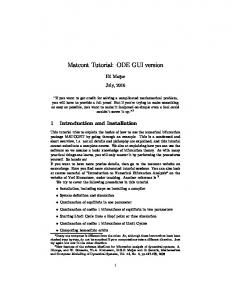
Figure 1: A typical matcont startup screen

Now several windows will open with a standard system called adapt2. A typical screenshot is shown in Figure 1. One window is titled matcont and has several menu options. For instance, to end your matcont session, choose ‘Select’ in the matcont window and then ‘Exit’. Hereafter we will indicate this with matcont:Select|Exit. Alternatively one clicks on the close button of the matcont window. 2

3

Equilibria in Jansen-Rit

In this tutorial we will investigate some simple equilibrium bifurcations in the Jansen-Rit model with an additional slow inhibitory component [2]. The model is given by  00 0 2   y000 + 2ay00 + a2 y0 = AaS(y1 − θy2 − (1 − θ)y3 )  y1 + 2ay1 + a y1 = Aa(II + C2 S(C1 y0 )) (1) 00 y + 2bf y20 + b2f y2 = Bf bf C4 S(C3 y0 )    200 y3 + 2bs y30 + b2s y3 = Bf bf C4 S(C3 y0 ) The sigmoidal function S is given by S(u) = 2 ∗ e0/(1 + exp(r ∗ (v0 − u))) and the constants satisfy C2 = 0.8C1 and C4 = C3 = 0.25C1 .

3.1

Specifying a new model

To specify the differential equations of the sytem click ‘(matcont):Select|Systems|New’ and a window titled ‘System’ appears with fields ‘Name system’, ‘Coordinates’, ‘Parameters’, ‘Time’, options for derivatives and a large box. The exact appearance of the System window depends on the operating system and the availability of the Matlab Symbolic Toolbox. If the latter is present, the lowest line will read ‘symbolically’. If possible, one should always choose to compute first,second and third order derivatives symbolically as this is the most reliable and fastest option. The first and second are mostly used in the continuation, the third order is useful for computing normal forms accurately. Go to www.math.utwente.nl/ meijerhge/MT.txt (or google Hil Meijer and go to my teaching page) for copy-pasting all the fields specified. Select symbolic derivatives up to order 3. You will have something like in Figure 2 and click ok.

Figure 2: Specifying a new model If you want to change the system or correct the input choose ‘(matcont):Select|Systems|Edit/Load’, select the system you want to edit and press ‘Edit’. Common mistakes(apart from simple typos): • Make sure not to put spaces between variables or parameters in their input fields • Make sure that multiplication is written explicitly with * or you get errors like ‘Unbalanced or misused parentheses or brackets’ or ‘error using ==> eval, Index exceeds matrix dimensions’. 3

• If your model has some strange behavior like ever increasing variables, check whether you have specified the differential equations in the same order as the order of the coordinates.

3.2

Time Simulations

Click ‘(matcont):Type|Initial point|Point’ to initialize the computation of an orbit starting from a point. In the matcont window the curve type is now P O, every curve type has a similar meaning. Two extra windows ‘Starter’ and ‘Integrator’ appear, the first is to specify initial conditions/points, the second to select the numerical integrator and change its settings. In the starter window set A = 3.25, a = 100, Bs = 8.8, bs = 20, Bf = 44, bf = 100, e0 = 2.5, r = 0.56, v0 = 6, theta = 0.5, CC = 220, II = 20. We also want to see how the orbits look like and for this we open a window ‘(matcont):Window|Plot|2D-plot’. In ‘Layout|Variables on axes’ select y0 as abscissa(standard) and y1 as ordinate, press ‘OK’ and let the axes range from -.1 to .1 for the abscissa and 0 to 3 for the ordinate using ‘(2Dplot:1):Layout|Plotting region’. In ‘Integrator’ change ‘Interval’ to 1 and ‘MaxStepsize’ to 0.1.

Figure 3: An orbit converging to a stable fixed point for CC = 220, II = 20. Left: (y0 , y1 )-phase plane, Right: simulation showing y0 (t). After these preparations we are ready to compute some orbits: Select ‘(matcont): Compute|Forward’. Starting from ~y = (y0 . . . , y7 ) = (0, . . . , 0) converges to (.0014, 1.79, 4.24, 4.24, 0, 0, 0, 0). You can monitor the orbit and its final values by opening via numeric window. Select ‘(matcont): Window|Numeric’ and recompute the orbit. You can try also other initial points and check that these also converge to this point. So we have a(n apparent) global attractor. To see how y0 evolves over time, select ‘(2Dplot:1): Layout|Variables on axes’ and select time and y0 . Redraw the curve via ‘(2Dplot:1): Plot|Redraw curve’ and adjust the plot-ranges to obtain Figure 3(right). Now change to II = 135 and again compute an orbit via ‘(matcont):Compute|Forward’. The result is quite different. You will have to adjust the axes to see the full range of y0 . You can use the pull-down menu as before, but the zoom-option (looking glass) in the menu bar is also useful, or manually from the command line with ylim([0 0.12]). The result should like Figure 4(right). We see some periodic behavior that has a frequency of 3Hz and looks like spike-wave discharge patterns seen in EEG.

3.3

Continuation of Equilibria in one parameter

We are now going to study the effect on the stability of the equilibrium when varying either II. Select the last point via ‘(matcont):Initial point’ and then choose the last point on the previous curve. 4

Figure 4: An orbit converging to a stable fixed point for CC = 220, II = 135. Left: (y0 , y1 )-phase plane, Right: simulation showing y0 (t).

Change the curve type to EP EP by selecting ‘(matcont):Type|Initial point|Equilibrium’. Activate the parameter II by clicking on the button next to it. In the 2Dplot:1 window change the abscissa to the parameter II via ‘(2Dplot:1):Layout|Variables on axes’. Also change the plotting region for II to -250 to 300 and for y0 to 0 to 0.1. To speed up the continuation we will set ‘Continuer):MaxStepsize=5’ ‘Continuer):MaxNumPoints=600’. The stability changes upon the variation of II thus we would also like to see how the eigenvalues of the Jacobian at the equilibrium develop. For this we select ‘(Numeric):Window|Layout’ and highlight the option ‘eigenvalues’( it changes to capitals). Since we have (too) parameters you may want to unselect the parameters (changes it to small letters). Press ‘OK’. Select ‘(matcont): Compute|Forward’. NOTE: In the lower left corner a small window appears with buttons ‘Pause’,‘Resume’ and ‘Stop’. Whenever a bifurcation is detected, MATCONT pauses and shows some relevant information. In the sequel a few such points will be detected, but we will not always indicate to resume the computation. At II = 109.388594 the message ‘Limit point’ appears in the status field of the matcont window. Here one eigenvalue has zero real part: Check that in the numeric window!. The curve(branch) of equilibria has a turning point, on one side the equilibria are stable on the other unstable. Press the ’Resume’ button in the lower left of your screen or press space to continue the computation of the now unstable branch. In the meantime MatCont find a special point, i.e. a test function is zero, but that is due to two real eigenvalues, one positive and one negative, summing up to zero, not a complex pair. This is mentioned in the main MatCont window as a neutral saddle. At II = −211.513481 another Limit point is found. Here the branch does not become stable, just one more eigenvalue has now positive real part. When II = −188.997488 is reached two complex conjugate eigenvalues have zero real part and a Hopf bifurcation occurs. The 2Dplot should now look like Figure 5. If the computation would be fast to follow, you can select to pause the computation of the EP EP curve after each computed point. For this choose ‘(matcont):Options|Pause|At each point’. (Do not forget to change it to ‘At special points’ after this computation. Now we turn to the command line, i.e. the Matlab window, where you most probably now have the following information:

first point found tangent vector to first point found label = LP, x = ( 0.010348 0.000000 6.716992 0.000000 5.517090 0.000000 5.517090 0.000000 109.388594

5

Figure 5: A branch of equilibria in the (II, y0 )-plane displaying co-existence and Hopf bifurcations.

a=6.161969e+001 label = H , x = ( 0.014027 Neutral saddle label = LP, x = ( 0.041898 a=-2.696137e+000 label = H , x = ( 0.047787 First Lyapunov coefficient label = H , x = ( 0.056467 First Lyapunov coefficient elapsed time = xxx secs npoints curve = 600

-0.000000 7.932056 0.000000 6.145333 0.000000 6.145333 0.000000 100.12128

-0.000000 17.675297 0.000000 13.563251 0.000000 13.563251 0.000000 -211.5

-0.000000 20.342252 0.000000 15.905967 0.000000 15.905967 0.000000 -188.9 = 7.016628e-005 0.000000 24.850741 0.000000 19.975932 0.000000 19.975932 0.000000 -91.880 = -2.370306e-004

The first two lines indicate that the continuation has started, and the last two that it has ended together with the number of points computed and the duration (including waiting time). Any other messages are displayed here, for instance the four bifurcations together with their normal form coefficients. This information is useful as it indicates the non-degeneracy and criticality of the bifurcations. First, the two Limit Point bifurcations are shown, x indicates the eight variables ~y and the value of the active parameter II at the bifurcation point. Then the normal form coefficients are given, note that for a Limit Point the sign of this coefficient is not unique (Why?). Finally, we know that the limit cycle born from the first and second Hopf bifurcation are unstable and unstable as the first Lyapunov coeffiecient is positive and negative, respectively. For further reference we will rename this curve so that it is not overwritten. Select ‘(matcont):Curve|Actions|Rename and give the computed curve EP EP(1) an other name, say ’steadystates’.

3.4

Continuation of Bifurcations of Equilibria in one parameter

Figure 5 showed a phenomenon called hysteresis or bistability. This is an important feature of nonlinear (differential) equations. In parameter space regions of bistability are usually delimited by a wedge of Limit point bifurcations which we will compute here.

6

Select one of the Limit points found in the equilibrium continuation as initial point ‘(matcont):Select|Initial point’. Activate II and CC as active parameters. Close the 3D-plot and re-open the 2D-plot. Change the ordinate of the 2D-plot to the parameter CC and its range from 0 to 250. Now select ‘(matcont):Compute|Forward’ and when finished also ‘Backward’. At (CC, II) ≈ (59.11, 168.7) a Cusp bifurcation (CP) and at (II, CC) = (1.6840517, 1.6829686) a spurious Zero-Hopf bifurcation is detected. You have now computed the wedge, see Figure 6 within which you have bistability. This is not the full story as we also found already Hopf bifurcations, implying that it is more co-existence and not bistability of equilibria.

Figure 6: Limit Point bifurcation curves in the (II, CC)-plane with codimension 2 points with a wedge of co-existence of equilibria.

To compute a curve of Hopf bifurcations: select a Hopf point analogously as for the Limit point as initial point. Change the curve type to H H via ‘(matcont):Type|Curve|Hopf’. Take here II and CC as active parameters. Press ‘Compute|Forward’ and ‘Compute|Backward’ to obtain the diagram as in Figure 7.

4 4.1

Continuation of Limit Cycles Starting from a Hopf point

We are now going to compute a branch of limit cycles starting from the Hopf point. Select the second Hopf point of the curve ‘equi’ using ‘(matcont):Select|Initial point’ as new initial point. Activate the parameter II and the period by clicking on the buttons in the Starter window. Next we select ”yes” for Fold under the heading monitor singularities in the starter window. By default, and for good reasons (many spurious warnings otherwise), detection of bifurcations is switched off. To speed up computations we will set MaxStepsize=200. This is large, but for this tutorial this is acceptable. Close the 2DPlot (for speed reasons: plotting the cycles takes too much time now) and ‘(matcont):Compute|Forward’. At II = 60.61 we see a Fold bifurcation and the periodic orbit becomes unstable. Resume the computation and stop when you are near II = −188. Here the branch terminates in the subcritical Hopf bifurcation. Open a 3D plot with ‘(matcont):Window|Plot|3D-Plot’. Choose

7

Figure 7: Limit Point and Hopf bifurcation curves in the (II, CC)-plane with codimension 2 points. The ZH is spurious, the GH indicates where the Hopf bifurcation changes from subto supercritical. The Hopf curve emerges from a Bogdanov-Takens point. To detect the lower BT-point, you should set the MaxStepsize to 0.05 in the Continuer window.

OX=z, OY=F , OZ=y in the draw3 attributes window. Change the plotting the region to II ∈ [−200, 100], y0 ∈ [0, .15], y1 ∈ [0, 30]. Your 3D-plot will resemble the one in Figure 8.

Figure 8: Equilibria and Limit cycles in (II, y0 , y1 )-space. The points and limit cycles which undergo a bifurcation are indicated with red dots.

8

4.2

Starting Limit Cycle from a time simulation

The continuation starting from the Hopf bifurcation worked, but it takes forever before the branch of periodic orbits comes to a relevant parameter regime, i.e. II > 70. In fact, it did not even get there at all. On the other hand, we already found an interesting periodic orbit and we will use that one to start the continuation directly in the interesting parameter regime. We will first recompute the periodic dynamics. Take ~y = 0 as initial condition and set II = 135. Set the point type matcont:Type|Point and press matcont:Compute|Forward. Now at the bottom of the starter window we see a tempting button Select Cycle. We cannot yet push it. What the algorithm does is to find the point of the trajectory nearest to the initial value. If it finds one, it takes that the time between these points as the period and fits a mesh to the computed solution. We proceed as follows: matcont:Select|Initial point and select the last point on the curve we have just computed. In integrator window change the interval to 0.4, which is an appropiate upper limit of the period. Press matcont:Compute|Forward. Select Plot|Clear and Plot|Redraw curve to see that it is a periodic orbit. Now press the Select Cycle button in the starter window. A popup will appear with two fields: ”Tolerance” equal to 1e-2 and ”test intervals” equal to 20. Change test intervals to 40 and press OK. Tick the boxes for II and Period as free parameters in the new starter window. Change MaxStepsize to 200 in the Continuer window. Open a Window|Numeric window and close the figure. Press matcont:Compute|Forward. Most likely, you will notice in the numeric window that II is decreasing while the period goes up. Around II ≈ 110 the period still goes up but II only slightly decreases. Here the periodic orbit gets close to a homoclinic orbit and it cannot be continued further. Rename the computed curve to lc1. Now we compute the other part of the branch, but first we select ”yes” for Fold under the heading monitor singularities in the starter window. By default, and for good reasons (many spurious warnings otherwise), detection of bifurcations is switched off. Press matcont:Compute|backward. You will observe two Fold bifurcations at II = 169.7 and II = 162.2. We can also inspect the eigenvalues and conclude that here we have a region of bistability again. The continuation then just runs and II increases, so you just might as well stop it. Rename the computed curve to lc2.

4.3

Continuation of LPC in two parameters

Similar to the fold and Hopf bifurcations of equilibria we want to compute the curves in parameter space where the dynamics changes. So select one of the computed LPC’s as initial point ‘matcont:Select|Initial Point’. Next set II and CC as active parameters and ‘matcont:Compute|Forward’. You can monitor the result via the Numeric window or a 2Dplot.

5

Visualizing your output

We have already plotted some of the computations. It is also possible to load the output and plot and manipulate it yourself. We will give a nontrivial example of plotting the profile. First we need to access the computed curves. In the matcont directory, there is a subdirectory called ‘Systems/JR slow/diagram’. Here we can find the file ‘lc2.mat’. Load the curve into the matlab workspace by entering on the command line: ‘load Systems/JR slow/diagram/lc2.mat’. Now your workspace contains five variables x, v, h, f, s. They contain the following data x Array containing the phase variables and parameters. v Array containing the tangent vector. h Array containing the stepsize, Newton steps and values of testfunctions. f Array containing eigenvalues or Floquet multipliers and the time discretization.

9

s A structure that specifies special points, i.e. detected bifurcations and the first and last point.

5.1

Plotting the profile

To plot the profile, i.e. the evolution of a variable during the whole period, is nontrivial as it is stored in a condensed way. Suppose we know how many mesh-points were used. This can be determined from the f variable, simply look up the first entry equal to 1. Now we need • the index of the periodic orbit we want to plot: say ii. • the profile of one variable, say the jj-th: x(jj:ndim:end-2,ii) • the time-mesh tau=f(1:ntst+1,ii), with 0 = τ0 < τ1 < ... < τntst = 1. • the period T= x(end-1,ii) to scale the mesh back from [0,1] to [0,T] So we could plot: ii=50;jj=1;ntst=40;ndim=8; plot(f(1:ntst+1,ii)*x(end-1,ii),x(jj:ndim:end-2,ii)) You will get an error message because the computed curve x contains also data about the orbit between mesh-points. While you are trying to plot the profile only coarsely at the mesh-points. A first correction would be ii=50;jj=1;ndim=8;ntst=40;ncol=4; plot(f(1:ntst+1,ii)*x(end-1,ii),x(jj:ndim*ncol:end-2,ii)) This is usually not good enough, so we actually want the detailed grid. For this we need to know j that between to mesh-points the orbit is stored at equi-distant time-points ti,j = ti + m (τi+1 − τ ), j = 0, 1, ..., m. So the correct commands are: ii=10;jj=1;ndim=8;ntst=40;ncol=4; mesh=sort([reshape(repmat(f(1:ntst,ii),1,ncol)+... repmat((0:ncol-1)/ncol,ntst,1).*repmat(diff(f(1:ntst+1,ii)),1,ncol),ntst*ncol,1); 1]); plot(mesh*x(end-1,ii),x(jj:ndim:end-2,ii))

5.2

Identifying Spike Wave Discharges

One particular feature of this model as that it has Spike-Wave Dynamics. That is, on top of the 3Hz wave, there is an additional spike that can be detected as a local extremum. This is also called a ‘false’-bifurcation. Here we will compute these local extrema. load Systems\JR_slow\diagram\lc1.mat out=x(3:8:end-2,:)-(x(5:8:end-2,:)+x(7:8:end-2,:))/2; extrema=nan(6,size(out,2)); for i=1:size(out,2) diff_tr=diff(out(1:end-1,i)); diff_tr_shift=diff(out(2:end,i)); temp=[out(find([ (diff_tr>0).*(diff_tr_shift