Material Optimization - Universität Stuttgart

53 (2010)

Universität Stuttgart Institut für Baustatik und Baudynamik

Junji Kato

Material Optimization for Fiber Reinforced Composites applying a Damage Formulation

Junji Kato

Material Optimization for Fiber Reinforced Composites applying a Damage Formulation

von

Junji Kato

Bericht Nr. 53 (2010) Institut f¨ ur Baustatik und Baudynamik der Universit¨at Stuttgart Professor Dr.-Ing. habil. M. Bischoff Stuttgart 2010

c Junji Kato  Berichte k¨onnen bezogen werden ¨uber: / Reports are distributed by: Institut f¨ ur Baustatik und Baudynamik Universit¨at Stuttgart Pfaffenwaldring 7 D-70550 Stuttgart Tel.: ++49(0)711/685 66123 Fax: ++49(0)711/685 66130 http://www.ibb.uni-stuttgart.de

¨ Alle Rechte, insbesondere das der Ubersetzung in andere Sprachen, vorbehalten. Ohne Genehmigung des Autors ist es nicht gestattet, diesen Bericht ganz oder teilweise auf photomechanischem, elektronischem oder sonstigem Wege zu kommerziellen Zwecken zu vervielf¨altigen. All rights reserved. In particular, the right to translate the text of this thesis into another language is reserved. No part of the material protected by this copyright notice may be reproduced or utilized in any form or by any means, electronic or mechanical, including photocopying, recording or by any other information storage and retrieval system, without written permission from the author.

D93 - Dissertation an der Universit¨at Stuttgart ISBN 978-3-00-030186-5

Material Optimization for Fiber Reinforced Composites applying a Damage Formulation Von der Fakult¨at Bau- und Umweltingenieurwissenschaften der Universit¨at Stuttgart zur Erlangung der W¨ urde eines Doktors der Ingenieurwissenschaften (Dr.-Ing.) genehmigte Abhandlung

vorgelegt von

Junji Kato aus Osaka, Japan

Hauptberichter:

Prof. Dr.-Ing. Dr.-Ing. E.h. Dr. h.c. Ekkehard Ramm

1. Mitberichter:

Prof. Dr. techn. Ole Sigmund

2. Mitberichter:

Prof. Dr.-Ing. Kai-Uwe Bletzinger

Tag der m¨ undlichen Pr¨ ufung:

5. Februar 2010

Institut f¨ ur Baustatik und Baudynamik der Universit¨at Stuttgart Stuttgart 2010

Zusammenfassung In dieser Arbeit werden Materialoptimierungs-Verfahren f¨ ur faserverst¨arkte Verbundwerkstoffe vorgestellt, insbesondere f¨ ur neuartige Faser-/Textilbetone. Diese Werkstoffe sind aus einem Bewehrungsnetz aus langen Karbon- oder Glasfasern aufgebaut, das in eine feink¨ornige Betonmatrix eingelegt wird. Im Gegensatz zu herk¨ommlicher Stahlbewehrung sind Textilfasern korrosionsfrei. Aufgrund der hohen Alkalibest¨andigkeit trifft das auch auf alkaliresistente Glasfasern zu. Dies erlaubt die Herstellung von leichten, d¨ unnwandigen Verbundkonstruktionen. Die kritische Eigenschaft von Faserbeton ist ein eventuell spr¨odes Versagen aufgrund des spr¨oden Verhaltens beider Komponenten Beton und Fasern sowie des komplexen Verbundverhaltens. Diese Charakteristik stellt eine ideale Anwendung f¨ ur die Materialoptimierung dar, wobei bei vorgegebenem Faservolumen die maximale Duktilit¨at der Struktur als Zielfunktion dient. Hierzu reicht es nicht aus, den Optimierungsprozess auf einem linear-elastischen Materialmodell aufzubauen, da materielle Nichtlinearit¨aten ber¨ ucksichtigt werden m¨ ussen. Im Rahmen dieser Arbeit wird f¨ ur Matrix- und Fasermaterial ein gradienten-erweitertes, isotropes Sch¨adigungsmodell verwendet und f¨ ur deren Kombination ein diskretes Verbundmodell. Die Strukturantwort von Faserbeton h¨angt von verschiedenen Parametern ab, wie z. B. der Fasergr¨oße, -l¨ange, -position, -ausrichtung, Impr¨agnierung, Oberfl¨achenrauhigkeit und dem Material der Fasern. Von den Entwurfsvariablen werden f¨ ur die Optimierung die Dimensionierung der Fasern und die Faserposition als die einflussreichsten Parameter ausgew¨ahlt. Eine klassische Materialoptimierung verwendet meistens im Element “verschmierte” Fasern zur Optimierung der Faserausrichtung. Hier ist dieses Modell ist allerdings zu grob, um die oben genannten Parameter zu untersuchen. F¨ ur die Optimierung der Duktilit¨at von Faserbeton werden in dieser Arbeit drei Arten von Materialoptimierungs-Verfahren, die Mehrphasen-Materialoptimierung, die MaterialFormoptimierung und die Mehrphasen-Layoutoptimierung vorgestellt. Die Mehrphasen-Materialoptimierung legt die optimale Verteilung mehrerer Materialien innerhalb eines vorgeschriebenen Entwurfsraums bei festem FE-Netz fest. Diese Methode ¨ahnelt der Topologieoptimierung, insbesondere dem dort h¨aufig eingesetzten SIMPAnsatz. Hierbei werden die optimale Fasergr¨oße, Faserl¨ange und Kombination verschiedener Fasermaterialien ermittelt. Die Material-Formoptimierung verbessert die Duktilit¨at, indem die Fasergeometrie unabh¨angig vom festen FE-Netz variiert wird. Dabei vereinfacht die Verwendung einer “embedded” Finite-Elemente-Formulierung die komplexe Diskretisierung d¨ unner Fasern bei klassischen FE-Modellen. Die Mehrphasen-Layoutoptimierung ermittelt nicht nur die optimale Fasergeometrie, sondern gleichzeitig die optimale Fasergr¨oße und die Art des Fasermaterials. Diese Methode entsteht durch Kombination von Mehrphasen-Materialoptimierung und Material-Formoptimierung. Zur L¨osung des Optimierungsproblems werden gradienten-basierte Verfahren eingesetzt. Aufgrund ihrer numerischen Effizienz und Robustheit werden sowohl das Optimalit¨atskriterien-Verfahren als auch das Verfahren der beweglichen Asymptoten verwendet. Die Sensitivit¨atsanalyse erfolgt durch analytische oder semi-analytische Verfahren. Das Verhalten der vorgestellten Methoden wird an einer Reihe von numerischen Beispielen untersucht, wobei die Duktilit¨at des Faserbetons wesentlich verbessert werden kann. Die vorgestellten Methoden zur Ermittlung optimaler Entw¨ urfe sind methodisch anspruchsvoll und vielversprechend und auch auf andere faserbewehrte Verbundwerkstoffe wie z. B. faserverst¨arktes Glas anwendbar.

Abstract The present thesis proposes material optimization schemes for fiber reinforced composites, specifically for a new composite material, denoted as Fiber Reinforced Concrete (FRC) or Textile Reinforced Concrete (TRC); here a reinforcement mesh of long carbon or glass fibers is embedded in a fine grained concrete (mortar) matrix. Unlike conventional steel reinforcement, these textile fibers are corrosion free; this holds also for AR-glass due to its high alkali-proof. This favorable property allows to manufacture light-weight thinwalled composite structures. However the critical aspect of this composite is that the structural response of FRC may show brittle failure due to the material brittleness of both constituents concrete and fiber in addition to their complex interfacial behavior. This specific characteristic of FRC is an ideal target for material optimization applying the overall structural ductility as objective which ought to be maximized for a prescribed fiber volume. For this objective it is of course not sufficient to base the optimization process on a linear elastic material model, so that it is mandatory to consider material nonlinearities. In the present study a gradient enhanced isotropic damage model is applied for both matrix and fiber materials and a discrete bond model is used for their interface. The structural response of FRC depends on several parameters, e.g. fiber size, fiber length, fiber location/orientation, impregnation, surface roughness of fiber, and the kind of fiber material itself. From these the most influential parameters like fiber dimensions and locations are chosen as design variables for optimization. Conventional material optimization applying simply ‘smeared-type elements’ mostly concentrate on the fiber orientation defined at each finite element. This approach is not detailed enough when the influence of other important parameters mentioned above ought to be investigated. Considering the design requirements for the present objective, this thesis proposes three kinds of material optimization schemes, namely multiphase material optimization, material shape optimization, and multiphase layout optimization. Multiphase material optimization determines an optimal distribution of several materials over a prescribed design domain in a fixed finite element mesh. This methodology is related to topology optimization, especially to the Solid Isotropic Microstructure with Penalization (SIMP) approach. With this method optimal fiber size, fiber length, and combination of different fiber materials can be obtained. The task of material shape optimization is to improve the structural ductility of FRC with respect to ‘fiber geometry’ which is independent of the fixed finite element mesh. By applying a so-called embedded finite element formulation, the complexity of discretization for thin fibers in a conventional finite element formulation is diminished. Multiphase layout optimization provides not only optimal fiber geometry but also optimal fiber size or the kind of fiber materials simultaneously. This methodology is achieved by combining above multiphase material and material shape optimization. For the optimization problems a gradient-based optimization scheme is assumed. An optimality criteria method and a method of moving asymptotes are applied considering their numerical high efficiency and robustness. For the sensitivity analyses variational direct analytical/semi-analytical methods are utilized. The performance of the proposed methods is demonstrated by a series of numerical examples; it is verified that the ductility of FRC can be substantially improved. The proposed methods providing optimal designs are promising and methodically challenging. They are also applicable to other fiber reinforced composites, for example Fiber Reinforced Glass (FRG).

Preface The present study was carried out at the Institute of Structural Mechanics of the University of Stuttgart within the research project FOR 509 ‘Multiscale Methods in Computational Mechanics’ in the German Research Foundation (DFG). In this context I gratefully acknowledge the financial support of the DFG. First of all, I would like to thank my supervisor Prof. Dr.-Ing. Ekkehard Ramm for his strong support to my study during the passed five years. It was in his wonderful lecture of the winter seminar for the international master program COMMAS at the University of Stuttgart in 2003 when I first met ‘structural optimization’. Even now I can remember how much impact I received from the lecture at that time. After my graduation from the master course, he kindly accepted me as one of his doctorands and also provided nice scientific environment. During the complete time period I learned a lot from him for not only scientific matters but also things personally very important in my life. Furthermore, I would like to thank Prof. Dr. techn. Ole Sigmund and Prof. Dr.-Ing. KaiUwe Bletzinger for their willingness to act as co-referees and their quick and accurate review of my thesis. Their advices as co-referees contributed to improve the quality of this dissertation. I would also like to thank Prof. Dr.-Ing. habil. Manfred Bischoff for his kind support and also his steady willingness to discuss various topics with me. The discussion and his advices played a significant role in this study and also have influenced my way of thinking as a researcher. I would like to express my thanks to all my colleagues of the Institute of Structural Mechanics for the ideal working conditions and the nice atmosphere. It is needless to say that their academic discussions, suggestions as well as the usual conversation have contributed to the outcome of the present study. I would also like to give special thanks to all my former colleagues of this institute, in particular, Michael Leukart, Gian Antonio D’Addetta, Frank Issler, Stefan Hartmann, Andrea&Tobias Erhart, and Andreas Lipka. I had an unforgettable, wonderful time with them here in Stuttgart. I would like to thank Mr. Sasaki, CEO of SIA Inc. Nagoya in Japan, for his cordial encouragements. His valuable and unerring advices also have still contributed to the improvement of my behavior and activity at international scenes. Finally, I would like to thank my dear family, especially my mother, for having been lavish with support. During the period of my doctor promotion a very sad thing happened in my family, a serious disease of my brother. Even under such a serious situation, she tried to behave cheerfully as usual and saw me off courageously to Germany. This thesis would not have been completed unless her support. I am very proud of being her son from bottom of my heart. Stuttgart, February 2010

Junji Kato

Contents Contents

i

Nomenclature

v

1 Introduction

1

1.1 Motivation . . . . . . . . . . . . . . . . . . . . . . . . . . . . . . . . . . . .

1

1.2 Scope and objective . . . . . . . . . . . . . . . . . . . . . . . . . . . . . . .

3

1.3 Outline . . . . . . . . . . . . . . . . . . . . . . . . . . . . . . . . . . . . . .

5

2 Fundamentals of structural optimization

7

2.1 Introduction . . . . . . . . . . . . . . . . . . . . . . . . . . . . . . . . . . .

7

2.2 Optimization model . . . . . . . . . . . . . . . . . . . . . . . . . . . . . . .

8

2.2.1

General . . . . . . . . . . . . . . . . . . . . . . . . . . . . . . . . .

8

2.2.2

Optimization method . . . . . . . . . . . . . . . . . . . . . . . . . . 11

2.3 Design model . . . . . . . . . . . . . . . . . . . . . . . . . . . . . . . . . . 16 2.3.1

Topology optimization . . . . . . . . . . . . . . . . . . . . . . . . . 17

2.3.2

Shape optimization . . . . . . . . . . . . . . . . . . . . . . . . . . . 19

2.4 Analysis model . . . . . . . . . . . . . . . . . . . . . . . . . . . . . . . . . 21 2.4.1

Finite element analysis . . . . . . . . . . . . . . . . . . . . . . . . . 21

2.4.2

Objective functions and constraints . . . . . . . . . . . . . . . . . . 24

2.5 Sensitivity analysis . . . . . . . . . . . . . . . . . . . . . . . . . . . . . . . 24 2.5.1

Overview . . . . . . . . . . . . . . . . . . . . . . . . . . . . . . . . 24

2.5.2

Discrete method . . . . . . . . . . . . . . . . . . . . . . . . . . . . . 26

2.5.3

Variational method . . . . . . . . . . . . . . . . . . . . . . . . . . . 28

3 Modeling of fiber reinforced composites

31

3.1 Overview of fiber reinforced concrete . . . . . . . . . . . . . . . . . . . . . 31 3.2 Material models . . . . . . . . . . . . . . . . . . . . . . . . . . . . . . . . . 35 3.2.1

Isotropic gradient enhanced damage model . . . . . . . . . . . . . . 35

i

ii

Contents 3.2.2

Discrete bond model for interface . . . . . . . . . . . . . . . . . . . 37

3.3 Alternatives for representations of reinforcement . . . . . . . . . . . . . . . 38 3.4 Kinematic assumption for embedded reinforcement formulation . . . . . . . 40 3.5 Finite element formulation of fiber reinforced composites . . . . . . . . . . 41 3.5.1

Virtual work . . . . . . . . . . . . . . . . . . . . . . . . . . . . . . . 41

3.5.2

Discretization . . . . . . . . . . . . . . . . . . . . . . . . . . . . . . 42

3.5.3

Element matrices . . . . . . . . . . . . . . . . . . . . . . . . . . . . 44

4 Design variables for optimization

45

4.1 Preliminary investigation for influential parameters . . . . . . . . . . . . . 45 4.2 Choice of design variables . . . . . . . . . . . . . . . . . . . . . . . . . . . 50 5 Sensitivity analysis for a materially nonlinear problem

51

5.1 Background . . . . . . . . . . . . . . . . . . . . . . . . . . . . . . . . . . . 51 5.2 Equilibrium formulation . . . . . . . . . . . . . . . . . . . . . . . . . . . . 53 5.3 Derivation of sensitivity analysis . . . . . . . . . . . . . . . . . . . . . . . . 53 5.4 Comparison between damage and plasticity models in sensitivity analysis . 56 6 Multiphase material optimization

59

6.1 Background . . . . . . . . . . . . . . . . . . . . . . . . . . . . . . . . . . . 59 6.2 Concept of multiphase material optimization

. . . . . . . . . . . . . . . . 60

6.3 Detailed concept of design variables . . . . . . . . . . . . . . . . . . . . . . 62 6.4 Interpolation rules and sensitivities . . . . . . . . . . . . . . . . . . . . . . 62 6.4.1

Basic model . . . . . . . . . . . . . . . . . . . . . . . . . . . . . . . 62

6.4.2

Two-phase material . . . . . . . . . . . . . . . . . . . . . . . . . . . 64

6.4.3

Three-phase material . . . . . . . . . . . . . . . . . . . . . . . . . . 65

6.5 Optimization problem . . . . . . . . . . . . . . . . . . . . . . . . . . . . . 67 6.6 Sensitivity analysis . . . . . . . . . . . . . . . . . . . . . . . . . . . . . . . 68 6.7 Numerical study on accuracy of sensitivity analysis . . . . . . . . . . . . . 68 6.8 Numerical examples . . . . . . . . . . . . . . . . . . . . . . . . . . . . . . . 70 6.8.1

Optimization with fiber length as design parameter . . . . . . . . . 71

6.8.2

Optimization considering fiber size and material combination . . . . 71

6.9 Discussion: Estimation of fitting parameter . . . . . . . . . . . . . . . . . . 74 6.10 Assessment of multiphase material optimization . . . . . . . . . . . . . . . 76

Contents

iii

7 Material shape optimization

79

7.1 Overview . . . . . . . . . . . . . . . . . . . . . . . . . . . . . . . . . . . . . 79 7.2 Concept of material shape optimization

. . . . . . . . . . . . . . . . . . . 79

7.2.1

Determination of intersections . . . . . . . . . . . . . . . . . . . . . 81

7.2.2

Inverse mapping for local coordinate of fiber . . . . . . . . . . . . . 82

7.3 Optimization problem . . . . . . . . . . . . . . . . . . . . . . . . . . . . . 82 7.3.1

Equilibrium conditions and total derivative of design function . . . 83

7.4 Sensitivity analysis . . . . . . . . . . . . . . . . . . . . . . . . . . . . . . . 83 7.4.1

Overview . . . . . . . . . . . . . . . . . . . . . . . . . . . . . . . . 83

7.4.2

Gradients of constitutive equations . . . . . . . . . . . . . . . . . . 84

7.4.3

Sensitivity for explicit term of objective function . . . . . . . . . . . 86

7.4.4

Sensitivity for first equilibrium equation . . . . . . . . . . . . . . . 87

7.4.5

Sensitivity for the second equilibrium equation . . . . . . . . . . . . 88

7.4.6

Sensitivity for the third equilibrium equation . . . . . . . . . . . . . 89

7.4.7

Total sensitivity . . . . . . . . . . . . . . . . . . . . . . . . . . . . . 90

7.5 Numerical examples . . . . . . . . . . . . . . . . . . . . . . . . . . . . . . . 91 7.5.1

Optimization of deep beam

. . . . . . . . . . . . . . . . . . . . . . 91

7.5.2

Optimization of hanging deep beam . . . . . . . . . . . . . . . . . . 93

7.5.3

Optimization of splitting plate . . . . . . . . . . . . . . . . . . . . . 93

7.6 Assessment of material shape optimization . . . . . . . . . . . . . . . . . . 95 8 Multiphase layout optimization

97

8.1 Overview . . . . . . . . . . . . . . . . . . . . . . . . . . . . . . . . . . . . . 97 8.2 Concept of multiphase layout optimization . . . . . . . . . . . . . . . . . . 98 8.3 Multiphase material for embedded fiber . . . . . . . . . . . . . . . . . . . . 99 8.4 Interpolation rule for interface . . . . . . . . . . . . . . . . . . . . . . . . . 101 8.5 Optimization problem . . . . . . . . . . . . . . . . . . . . . . . . . . . . . 102 8.6 Sensitivity analysis . . . . . . . . . . . . . . . . . . . . . . . . . . . . . . . 102 8.6.1

Overview . . . . . . . . . . . . . . . . . . . . . . . . . . . . . . . . 102

8.6.2

Gradients of constitutive equations . . . . . . . . . . . . . . . . . . 102

8.6.3

Calculation of sensitivity analysis . . . . . . . . . . . . . . . . . . . 104

8.6.4

Total sensitivity . . . . . . . . . . . . . . . . . . . . . . . . . . . . . 105

8.7 Numerical examples . . . . . . . . . . . . . . . . . . . . . . . . . . . . . . . 106 8.7.1

Material shape optimization v.s. multiphase layout optimization . . 106

8.7.2

L-shape plate . . . . . . . . . . . . . . . . . . . . . . . . . . . . . . 109

iv

Contents 8.8 Assessment of multiphase layout optimization . . . . . . . . . . . . . . . . 113

9 Conclusions

115

9.1 Summary . . . . . . . . . . . . . . . . . . . . . . . . . . . . . . . . . . . . 115 9.2 Outlook . . . . . . . . . . . . . . . . . . . . . . . . . . . . . . . . . . . . . 116 A Supplement of embedded reinforcement formulation

117

A.1 Transformation matrices . . . . . . . . . . . . . . . . . . . . . . . . . . . . 117 A.2 Linearization of gradient enhanced damage model for concrete . . . . . . . 117 A.3 Linearization of gradient enhanced damage model for fiber . . . . . . . . . 118 A.4 Linearization of interface element . . . . . . . . . . . . . . . . . . . . . . . 119 B Inaccurate sensitivity in semi-analytical method

121

C Material properties of interface model

125

References

127

Nomenclature The following abbreviations and symbols will be addressed several times throughout the thesis. Additionally, rarely occurring abbreviations and symbols are noted in the corresponding context. Abbreviations CAD CAGD CARAT CCARAT FE FEM OC MP MMA SQP PVW

Computer Aided Design Computer Aided Geometric Design Computer Aided Research and Analysis Tool - FEM Program system C-programming version of CARAT Finite Element Finite Element Method Optimality Criteria method Mathematical Programing method Method of Moving Asymptotes Sequential Quadratic Programming method Principle of Virtual Work

Symbols ( ˆ• ) ( •˙ ) ( • )∗ ( • )h ( • )(k) ( • )(n) ( • )t+1 ( • )t ( • )e ( • )s ( • )x ( • )y ( • )c ( • )f ( • )i ( • )c+f δ(•) d(•)

free function parameters time derivatives solution of optimization problem, values at optimum approximate function iteration index in optimization algorithms iteration index in path-dependent algorithms values at the actual time step values at the reference (previous) time step values on element level values of optimization vector component of x-direction vector component of y-direction term relevant to concrete matrix term relevant to fiber term relevant to interface between matrix and fiber term relevant to concrete matrix and fiber variation infinitesimal increment

v

vi Δ(•)

Nomenclature increment value

Gradient operators ∇s ( • ) ∇ex s (•) ∇imp (•) s 2 ∇

partial derivatives with respect to an optimization variable ˆsi , by which other variables ˆsj for j = i are regarded as constant explicit part of partial derivatives ∇s ( • ) implicit part of partial derivatives ∇s ( • ) Laplacean operator

Function spaces, mathematical functions L∞ (Ω) R Z V • •

Lebesgue space set of all real numbers set of all integer numbers subspace L2 norm Macauley bracket

Optimization values, functions L f h g h g s ˆs sr ˆsr sg ˆsg ˆsL , ˆsU η γ μ ns nf nh ng ng, active ζ

Lagrangian function objective function equality constraint inequality constraint vector of equality constraints vector of inequality constraints design function, design variable vector of optimization variables design function for material design vector of material design variables design function for shape design vector of shape design variables lower and upper bounds of optimization variables vector of the Lagrange multipliers for equality constraints vector of the Lagrange multipliers for inequality constraints adjoint vector/vector of the Lagrange multipliers number of design variables number of objective functions number of equality constraints number of inequality constraints number of active inequality constraints effective material parameter for damage

Geometry B Φ ϑ

material body shape function of geometry local coordinate of design element or of fiber geometry

Nomenclature χ Ω Ωe Ωϑ Ωξ Γ Γu Γσ Γe Γξ x xk xe J |J| ˜ J ˜ |J| N ˜ N ¯ N

vii

indicator function volume, design space subspace on element level subspace on local coordinate ϑ subspace in natural coordinate system boundary displacement boundary traction boundary boundary on element level boundary in natural coordinate system position vector of material point in actual configuration position vector of control nodes position vector of FE-nodes Jacobian matrix determinant of Jacobian matrix metric tensor determinant of metric tensor matrix of shape function for displacement vector field matrix of shape function for non-local equivalent strain field matrix of shape function for interfacial slip field

Kinematic measures u uL ε εL εL εa εpre d e ¯ d L B ˜ B ¯ B I1 J2

displacement vector field local displacement field along axis of one-dimensional fiber stain tensor stain tensor in local coordinate system local strain field along axis of one-dimensional fiber adjoint strain tensor prescribed strain nodal displacement vector nodal non-local strain vector nodal slip vector (nodal relative displacement vector) differential operator discretized constant differential operator for displacement field discretized constant differential operator for non-local equivalent strain field discretized constant differential operator for interfacial slip field first invariant of the strain tensor second invariant of the deviatoric strain tensor

Forces, loads, stresses σ σL σL t ˆt t0

Cauchy stress tensor Cauchy stress tensor in local coordinate system local stress along axis of one-dimensional fiber Cauchy traction vector prescribed surface traction vector reference surface traction vector

viii ˆ b P Ppse Fint Fext λ

Nomenclature prescribed body force vector per unit volume external load vector pseudo load vector internal force vector external force vector load factor

Works, stiffness matrices Wint Wext δW δWu δWe K KT

internal work external work virtual work part of virtual work relevant to displacement field part of virtual work relevant to non-local equivalent strain stiffness matrix tangential stiffness matrix

Materials C, Cel Ced CT Td Tε Tσ ρ θ E ν κ0 α β k D κ η ηˆ εv ε˜v c ui1 , ui2 , ui3 kL σm, 0 , σm σf, 0 , σf rs h αr , αf fc

elastic material stiffness tensor or matrix elasto-damage secant material stiffness tensor or matrix tangential material stiffness tensor or matrix rotation matrix strain transformation matrix stress transformation matrix density angle Elastic modulus Poison’s ratio threshold variable which determines damage initiation softening parameter which defines final softening stage softening parameter which governs rate of damage growth ratio of compression relative to the tension strength damage parameter history variables of damage penalization factor fitting parameter local equivalent strain non-local equivalent strain dimension length squared regularizing localization of deformation slip length defining change of interfacial behavior tangential stiffness of interface initial and current adhesion strength initial and current sliding friction strength fiber radius surface roughness of a fiber constants assuming lateral deformation of fiber uniaxial compressive strength of concrete

Nomenclature εs Rs σR

uniaxial strain of fiber radius of curvature at slip ui1 stress perpendicular to fiber

Optimization method Ys Yη , Yγ  ¯ β, β Li , Ui α ˜

iteration rule for optimization variables (OC method) iteration rule for Lagrange multiplier (OC method) shift factor (OC method) stop criterion (OC method) move limits for i -th design variable (MMA) lower and upper asymptotes for i -th design variable (MMA) variation for asymptotes (MMA)

ix

Chapter 1 Introduction 1.1

Motivation

Optimal design has always been a common interest for engineers in all fields. Engineers usually make every effort to come up with the optimal design in terms of their experience, knowledge, engineering sense and of course the theoretical background as the basis for structural analysis. In this approach mechanical principles are applied to determine the structural response, for example deflections and stress states, while loads, boundary conditions, and geometry of a structure, i.e. topology and shape of a structure, are given. However in the case in which the structural problem is highly nonlinear or in which the objective to be requested is beyond human/engineering experience, the traditional approach does not provide necessarily reasonable optimal designs. In the meanwhile the mechanical laws can also be used to determine the conceptual layout, topology and shape of a structure, for a prescribed structural response. This inverse method is called structural optimization. With respect to optimization variables, structural optimization is usually divided into four levels which differ in their degree of complexity, in particular topology optimization, shape optimization, section sizing optimization, and material optimization, see Fig. 1.1. The task of the topology optimization is to generate a first ideal structural layout. Once the topology is determined, the external and/or internal boundaries may be varied to meet the mechanical requirements. This is the task of shape optimization. As the lowest level of structural optimization, sizing and material optimization contributes to the final topology optimization

shape optimization

sizing optimization

material optimization

Figure 1.1: Levels of structural optimization (Ramm et al. [149])

1

2

Chapter 1. Introduction

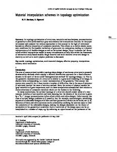
Figure 1.2: FRC pedestrian bridge (Curbach & Jesse [50]), FRC thin plate and textile fiber mesh (Brameshuber et al. [34]), textile fiber in concrete matrix (Hund [85])

detailing of a given structure; for instance, for cross sectional size of structural members or orientation of fibers in composites. Due to their different complexities, the individual classes of optimization have reached different stages of application. Sizing and material optimization is still the most advanced class while shape optimization and in particular topology optimization have been developed extensively and may already be standard design tool today. Of course, some ideas are still in the developing phase. In this study structural optimization is applied to fiber reinforced composites, specifically a new composite material, Fiber Reinforced Concrete (FRC), often called Textile Reinforced Concrete (TRC). The most widely used fiber reinforced composites are Fiber Reinforced Polymers (FRP), where often long glass, carbon or aramid fibers are placed into a polymer matrix leading to a good-natured ductile material. FRC differs from FRP in that the fibers are placed in a fine grained concrete or mortar matrix, often as a reinforcement mesh with a relatively low fiber content. Unlike conventional steel reinforcement, this kind of textile fiber is corrosion free due to its high alkali-proof; this property allows for the manufacturing of light-weight thin-walled composite structures, see Fig. 1.2. Nowadays the developments of FRC with long textile reinforcement may be a major concern for that long fibers oriented in the direction of tensile stress provide clearly higher strength than randomly oriented short fibers. This new composite material has received attention in civil engineering due to its great advantage and new possibilities involved. However the critical aspect of this composite is that the structural response of FRC shows brittle failure behavior due to material brittleness of both concrete and fiber in addition to complex interfacial behavior between above constituents. Thus the failure mechanism of FRC is highly complex, e.g. influenced by matrix cracking, slip of filaments in a roving, debonding of fibers from matrix and breaking of fibers. The specific characteristic of FRC is an ideal target for material optimization applying the overall structural ductility as objective which ought to be maximized for a prescribed fiber volume. For this objective it is of course not sufficient to base the optimization process on a linear material model, so that it is mandatory to consider material nonlinearities. The structural response of FRC strongly depends on many parameters, e.g. fiber size, fiber length, fiber location/orientation, impregnation, surface roughness of fiber, and the kind of fiber material itself. For this case conventional material optimization applying ‘smeared-type elements’ is not sufficient because this approach concentrates more or less simply on the fiber orienta-

1.2. Scope and objective

3

tion defined at each finite element and has less flexibility to deal with other parameters mentioned above. Furthermore this approach often results in discontinuous fiber representations between adjacent elements, namely incompatible fibers, which are unfavorable to consider realistic structural behavior especially for nonlinear structural response. Consequently, these two demands motivate the development of a new class of material optimization schemes based on the material nonlinearities which can provide a design flexibility. However the development of material optimization encounters extra challenges underlying in the modeling of fiber reinforced composites. One of the difficulties is the spatial discretization. The thickness of fibers is in general very small and constant along the fiber length; this requires ‘fine’ discretization if a conventional FE-mesh is used, and also provides a strict constraint to the thickness in the discretization process. Another difficulty is on the evaluation of the interface model between two constituents. The analysis model may become quite complex depending on the interface model adopted. Unlike the well-developed ‘topology optimization’ or ‘shape optimization’, material optimization is still in academic phase caused by these problems.

1.2

Scope and objective

The first objective of this thesis is to develop a potential new class of material optimization scheme which can substantially improve the structural ductility of FRC. In the present study the structural ductility means energy absorption capacity, which is measured by integral of the area below the stress-strain curve along the entire structure. The design variables investigated in this study are not only fiber orientation but also fiber size, fiber geometry (fiber length, location) and combination of different fiber materials. In order to consider the realistic structural response of FRC, the nonlinear failure behavior of matrix, fiber, and interface is considered. With respect to the selected design variables, the following three kinds of material optimization schemes are proposed, namely ‘multiphase material optimization ’, ‘material shape optimization ’ and ‘multiphase layout optimization’. Each method is briefly described as follows: • Multiphase material optimization : The task of the present methodology is to determine an optimal ‘multiple’ material distribution over a prescribed design domain, denoted as ‘design element’, for example a layer in the structure of Fig. 1.3. This methodology is strongly related to topology optimization, especially to the Solid Isotropic Microstructure with Penalization of intermediate densities for a one-phase material, the so-called SIMP approach (Bendsøe et al. [18]; Zhou & Rozvany [213]). Each finite element in the design element has properties of a smeared material, depending on the ‘mixture’ of the constituents. Material parameters of the design element are controlled by the volume fraction of the constituents. In this study, fiber length, fiber size, and combination of different fiber materials are chosen as the design variables. • Material shape optimization The purpose of this methodology is to improve the structural ductility of FRC with respect to ‘fiber geometry’ which is independent of the fixed Finite Element mesh.

4

Chapter 1. Introduction matrix

mixture

fiber material

(a) original

design element layers

(b) optimized

Figure 1.3: Concept of multiphase material optimization , (a) original and (b) optimized structures fiber: discontinuous

fiber: continuous Q anisotropic material

(a) conventional approach

(b) material shape optimization

Figure 1.4: Concept of material shape optimization , (a) conventional approach for fiber orientation and (b) material shape optimization

This methodology makes it possible to represent ‘continuous long’ fibers by applying a so-called embedded finite element formulation, which are more physically realistic than discontinuous fiber distributions resulting from the application of a conventional material optimization scheme, see Fig. 1.4. The fiber geometry is approximated by continuous functions such as B´ezier-splines; the coordinates of control points of the functions are chosen as design variables. Therefore, this methodology is based on shape optimization. • Multiphase layout optimization The purpose of the third methodology is to determine not only optimal fiber geometry but also fiber size or the kinds of fiber materials simultaneously for a prescribed fiber volume. This method is achieved by combining multiphase material optimization and material shape optimization . In material shape optimization strict restrictions are present in the design process, e.g. each fiber size is invariant and the number of fiber does not change during optimization process. These restrictions may lead to an unexpected local minimum, which is a consequence of the underlying non-convex optimization problem. As a result structurally ‘unexploited’ fibers may appear in the final optimal design, see Fig. 1.5 (a). The present methodology improves this problem by varying each fiber size. The size of structurally significant fibers becomes larger while the unexploited fibers may result in ‘zero-thickness’ which does not have any mechanical property. Consequently, this method may eliminate the unexploited fibers from the final optimal structure and provides a more

1.3. Outline

5

fiber thickness: invariant (unexploited fiber)

(a) material shape optimization

fiber thickness: variable (zero thickness)

(b) multiphase layout optimization (multiphase material + material shape)

Figure 1.5: Concept of multiphase layout optimization, (a) material shape optimization and (b) multiphase layout optimization

consistent design than material shape optimization. Second focal point is how the nonlinear structural response of FRC is considered in sensitivity analysis. A large amount of research effort has been devoted to the development of optimal design process for structural problems with linear structural response. This is mainly due to the fact that most often structures have been designed and used in a linear elastic range. However increasing attention to the use of new materials having nonlinear properties and the design requirement for structures to survive under severe conditions urge the development of optimal design processes considering nonlinear structural response. Nonlinear structural response is often distinguished between path-independent and pathdependent problems. In general if structural response is path-dependent, its sensitivity analysis also has to be path-dependent. For example path-dependent sensitivity analysis is discussed using plasticity models. In this study path-dependent sensitivity analysis is utilized for a damage model. The difference between damage and plasticity models in sensitivity analysis is also described.

1.3

Outline

The present thesis consists of nine chapters and each chapter is headed by general introductory remarks which include a summary of relevant literatures. The text is organized mainly by four parts. In the first part, the fundamentals of structural optimization are introduced, where the general formulations of optimization model, design model, analysis model, and sensitivity analysis are described (chapter 2). In chapter 5 the description of sensitivity analysis for a materially nonlinear problem is shown. In particular the derivation of sensitivities for a damage model is extensively discussed; this assists the comprehension of the complex sensitivity analyses involved in chapters 6 to 8. In the second part, the characteristics of textile reinforced concrete and its modeling are presented (chapter 3). Firstly, the applied material models are introduced. Secondly, the representation of reinforcement for fiber reinforced composites is discussed, where the following three kinds of formulations are introduced, a discrete reinforcement element, a smeared element, and an embedded reinforcement element. The discrete reinforcement

6

Chapter 1. Introduction

formulation is used in chapter 6 and the embedded reinforcement element is applied in chapters 7 and 8, respectively. As the embedded reinforcement element is based on a specific assumption, its description is given in sections 3.4 and 3.5. Some details are shifted to the Appendix A, e.g. the transformation matrices relevant to the fiber orientations and the linearization of the model. In the third part, design variables for the present optimization problem are discussed (chapters 4). As mentioned in the previous section, the structural response of FRC depends on several kinds of parameters. Thus it is very important to identify influential key parameters on the structural response of FRC before starting a detailed optimization. The selected key parameters are to be used as design variables for the present optimization problem. Three kinds of material optimization schemes as defined above are proposed in the final part. In chapter 6 multiphase material optimization is presented, where the basic concept and the corresponding sensitivity analysis are described. In chapter 7 material shape optimization is mentioned, where special attention is paid to the concept of global layout of fiber geometry and the procedure to define the fiber geometry. In chapter 8 multiphase layout optimization is introduced, in which the basic idea of this method and the procedure to combine the aforementioned two optimization methods are described. In these three chapters, the performance of the proposed methods is demonstrated by corresponding numerical examples and advantages and disadvantages of each scheme are shown. A final valuation of the thesis’ content and a perspective on future work concludes the thesis in chapter 9.

Chapter 2 Fundamentals of structural optimization 2.1

Introduction

Mechanical principles are usually applied to determine the structural response, for example deflections and stress states, while loads, boundary conditions, and geometry of a structure, i.e. topology and shape, are given. However the mechanical laws can also be used to determine the conceptual layout (topology) and shape of a structure for a prescribed structural response. This inverse method is called structural optimization. Problems of optimal design can be traced back to the origins of structural mechanics. In 1638 Galileo Galilei (1564-1642) already dealt with an optimum shape of cantilever beams in his famous “Discorsi” (Szabo [188]). For the early developments of structural optimization, the first analytical work was done by Maxwell [121] in 1895, followed by the better-known work of Michell [126] in 1904. These two works introduced theoretical lower bounds on the weight of trusses. These early developments considerably influenced the subsequent researches of optimization. Afterwards, a very important generalization was made by Prager [145] and Rozvany & Prager [164]. These studies introduced a methodology based on optimality criteria using an analytical procedure (see Rozvany et al. [165]). However few academic optimization problems can be analytically solved. Therefore, today numerical methods are applied to approximate the optimization solution. This methodVariational formulation LĂ (x, Ă s, Ă u, Ă g, Ă h) Geometry s(x)

Approximation & discretization

Design model

Analysis model

s ǒx, Ă sǓ h

Structural response u(x)

u hǒx, Ă ^ sǓ

^

Optimization model LĂ ǒx, Ă ^ s, Ă ^ u, Ă g, Ă hǓ

Figure 2.1: Numerical modeling

7

8

Chapter 2. Fundamentals of structural optimization

ology is based on a discretization of the design function s(x) and the structural response, e.g. displacements u(x) s (x) ≈ sh (x) = sh (x, ˆs) ;

ˆ) . u (x) ≈ uh (x) = uh (x, u

(2.1)

ˆ are discrete variable parameters of piecewise smooth approximations sh The vectors ˆs, u and uh . According to the discretization three numerical models can be distinguished (see Fig. 2.1), • Optimization model: The original continuous problem is formulated as a parameter optimization problem based on the following design and analysis models. The set of problem is defined by objective function, constraints, and design variables. • Design model: The design model provides a connection between the optimization model and the following analysis model. Geometry or material properties of a structure are interpolated by numerical schemes. Based on a spatial discretization, the material properties or shape is approximated by local shape functions. For example, parameters of the shape functions such as coordinates of control nodes of splines are the typical optimization variables ˆs for shape optimization. • Analysis model: In structural optimization the finite element method is most often applied to deˆ and to evaluate the mechanically oriented design termine the structural response u criteria, e.g. objective function and constraints. The calculation of sensitivity, i.e. the gradients with respect to design variables ˆs, is of utmost interest. ˆ . Thus the optimization The optimization problem is in general nonlinear in ˆs and u solution is obtained by iterative methods. However most often the structural response ˆ is already determined within the analysis model in terms of efficient finite element u ˆ are eliminated in the optimization problem procedures. In this case, the state variables u and the optimization only determines the optimization variables ˆs. Optimization algorithms are applied at the final stage after each structural analysis in order to obtain a new set of design variables. The optimization problems are solved by numerical methods depending on the characteristics of the problems. The following sections are devoted to further explanations for the above three models.

2.2 2.2.1

Optimization model General

An optimization problem can be generally formulated as follows, min

f (ˆs)

; f (ˆs) ∈

R

h (ˆs) = 0

; h (ˆs) ∈

Rnh

g (ˆs) ≤ 0

; g (ˆs) ∈

Rng

ˆs = {ˆs ∈ Vs | ˆsL ≤ ˆs ≤ ˆsU }

(2.2)

2.2. Optimization model

9

where f (ˆs) is objective function, h (ˆs) , g (ˆs) are equality constraints and inequality constraints, respectively. The upper and lower bounds of the optimization variables ˆs are denoted by ˆsU and ˆsL . One can distinguish between a discrete optimization problem, where only discrete values of optimization variables can be accepted (Vs ⊂ Zns ), and a continuous problem (Vs ⊂ Rns ). The optimization problem is called linear programming if all equations in Eq. (2.2) are linear in ˆs, while it is called nonlinear programming if the objective function or the constraints or both contain nonlinear parts. Whether or not the design criteria are smooth with respect to optimization variables ˆs is a significant distinction. The smooth optimization problem is reduced to a system of nonlinear equations in ˆs which can be solved by mathematically or mechanically oriented optimization algorithms, such as mathematical programming or optimality criteria methods, i.e. gradient-based methods. Non-smooth (discrete) optimization problems, like integer problems, can be solved by stochastic schemes such as evolutionary strategies or genetic algorithms, i.e. gradient-free methods. All optimization problems introduced in the present study are categorized as nonlinear smooth constrained optimization problems. For the basic knowledge to solve linear and nonlinear constrained problems it can be referred to the books by Gill et al. [64], Kirsch [96] and Haftka et al. [68]. Notion of local and global minima In constrained optimization problems the feasible domain of optimization variables is determined by the existing constraints. Fig. 2.2 (a) shows a simple situation of a constrained problem with two optimization variables. In general the global minimum under a constrained problem differs from that of the unconstrained problem. In many cases the optimization problem shown in Eq. (2.2) may have several local minima. Existence of a single global minimum could be assured only under special circumstances. Most often the local and global minima stay on the boundary of the active constraints. The local or global minima are mathematically determined by the important necessary conditions for optimality, so-called the Karush-Kuhn-Tucker (KKT) conditions, often only referred to as Kuhn-Tucker conditions. Lagrangian function and Kuhn-Tucker conditions The necessary conditions for a minimum of the constrained problem are obtained by applying the Lagrange multiplier method. The Lagrangian function is defined as follows, L (ˆs, η, γ) = f (ˆs) + η T h (ˆs) + γ T g (ˆs) → stationary.

(2.3)

The vectors η ∈ Rnh and γ ∈ Rng are defined as the Lagrange multipliers. The stationary value of Lagrangian function L (ˆs∗ , η ∗ , γ ∗ ) stays at a saddle point in (ns + nh + ng ) dimensional space, L (ˆs∗ , η, γ) ≤ L (ˆs∗ , η ∗ , γ ∗ ) ≤ L (ˆs, η ∗ , γ ∗ ) .

(2.4)

For the variables of the Lagrangian function, ˆs is called the primary variable and η, γ the dual variables. The necessary Kuhn-Tucker conditions for the saddle point are derived

10

Chapter 2. Fundamentals of structural optimization

from the partial derivative of the Lagrangian function with respect to the primal and dual variables. If ˆs∗ is a local minimum, then there exist the vectors of the Lagrange multipliers η, γ such that ∇s f (ˆs∗ ) + η T ∇s h (ˆs∗ ) + γ T ∇s g (ˆs∗ )

= 0

h (ˆs∗ )

= 0

γj∗

∗

gj (ˆs )

(2.5) ∗

= 0 with gj (ˆs ) ≤ 0,

γj∗

≥ 0.

Since g (ˆs∗ ) ≤ 0 and γ ∗ ≥ 0 it follows that if the j-th inequality constraint gj (ˆs∗ ) is non-zero then the corresponding γj∗ is zero. Any component of g (ˆs∗ ) which is zero is said to be an active constraint function at ˆs∗ . The geometrical interpretation of the KuhnTucker conditions is illustrated in Fig. 2.2 (b) for the case of two constraints. ∇s g1 , ∇s g2 denote the gradients of the two constraints g1 , g2 and are orthogonal to the respective constraint surfaces. Here ∇s ( • ) (= ∂ ( •) /∂s) is the partial derivative with respect to an optimization variable ˆsi , regarding other variables ˆsk for k = i as constants. s in the denominator of the partial derivative is the abbreviation for ˆsi . ˆs denotes a component of the design variable vector ˆs and is equivalent to ˆsi . s except the above abbreviation stands for a design function in this study. The negative gradient of objective function, i.e. (−∇s f) is defined by the linear combination of the gradients of the active constraints ∇s g1 , ∇s g2 for γj∗ ≥ 0. If the Kuhn-Tucker conditions are satisfied at the saddle point, it is impossible to find any direction which can further reduce the objective value f without violating the constraints. The sufficient condition for a local minimum requires the second derivatives of the Lagrangian function. Assuming that f, h, and g are twice differentiable functions with respect to ˆs, the sufficient condition for optimality is that the Hessian matrix of the Lagrangian function is positive definite:   ˜ T ∇2s L˜ ˜ ∈ Rns | v ˜ = 0, v ˜ T ∇s h = 0, v ˜ T ∇s gj = 0 with γ ∗j ≥ 0 . v v > 0 ; v (2.6) In some cases the necessary conditions are also sufficient for optimality. This is the case that the objective function and the inequality constraints are continuously differentiable y ^

s2

s2 unconstrained globalĂ minimum

(a)

^

s1

feasibleĂ domain

g1

^

globalĂ minimum feasibleĂ domain constraints

g2

ʼnsĂ f

^ ^ yĂ +Ă fĂ (s 1, Ă s 2)

localĂ minimum

ÉÉÉÉÉ ÉÉÉÉÉ ÉÉÉÉÉ ÉÉÉÉÉ ÉÉÉÉÉÉÉÉ ÉÉÉÉÉ ÉÉÉÉÉÉÉÉ ÉÉÉÉÉ ÉÉÉÉÉÉÉÉ ÉÉÉÉÉ Ă f min

g 1 ʼn s g 1 ) g 2 ʼn sg 2

fĂ increases ^

s1

(b)

Figure 2.2: (a) Notion of local and global minima and (b) Kuhn-Tucker conditions

2.2. Optimization model f

11 ^

^

f

^ f(s )

s2

s2

^

f(sU)

feasible domain

feasible domain

^ f(s L) ^ ^

^ sL sU (a)Ă convexĂ function

s

^ s ^ sL sU (b)Ă non * convexĂ function

^

s1

^

(c)Ă convexĂ domain

constraints

^

s1

(d)Ă non * convexĂ domain

Figure 2.3: Classification of functions and feasible domains on convexity, (a) convex function, (b) non-convex function, (c) convex domain, (d) non-convex domain

convex functions and the equality constraints are linear functions. This is the so-called convex optimization which guarantees any local minimum to be a global one. If a nonconvex equality constraint is present, then it always defines a non-convex feasible domain for the problem, i.e. this case is not a convex optimization problem (Kirsch [96]). In order to assist the above explanation the convex/non-convex functions and domains are visualized in Fig. 2.3.

2.2.2

Optimization method

Despite the variety of optimization strategies, it is possible to classify these strategies into the several groups. The traditional classification of optimization methods can be shown by referring to Venkayya [193] and Kirsch [96] as follows: • Mathematical Programing (MP) methods • Optimality Criteria (OC) methods • Stochastic methods The MP and OC methods are widely used for smooth optimization problems while the stochastic methods are often applied for non-smooth ones, such as integer optimization problems. The first two schemes are often called the gradient-based methods and the other is the gradient-free scheme. This classification can be quite nebulous because there can be a great deal of overlapping. For instance, the MP methods include linear, nonlinear, geometric and integer programming methods. The stochastic methods, e.g. the evolutionary strategies, simulated annealing or genetic algorithms, incorporate probabilistic (random) elements, either in the problem data (objective function, constraints) or in the algorithm itself, see Rechenberg [151]. As mentioned in section 2.2.1, the present thesis deals with nonlinear smooth constrained optimization problems. Therefore, the methods discussed in this section are devoted to the gradient-based schemes. First of all, the MP methods to solve nonlinear constrained structural optimization problems are described. The first work using the nonlinear MP method for constrained problems was introduced by Schmit [170] in 1960. Since then, many solution methods have been developed. The nonlinear MP methods for constrained problems can be categorized into indirect and direct approaches. Indirect approaches convert the problem first into

12

Chapter 2. Fundamentals of structural optimization

an equivalent ‘unconstrained’ optimization problem in terms of Lagrange multipliers or penalty parameters while direct approaches deal with the constrained formulation as it is. The representative indirect methods are, for example, the exterior/interior penalty function methods and the augmented Lagrange multiplier method. In the meanwhile the direct methods often used are the feasible direction method, the dual method, the gradient projection and reduced gradient methods. These methods were attractive due to the generality and rigorous theoretical basis. However there was a drawback that the application of the MP method was limited to relatively small optimization problems due to its high computational efforts and time consumption. One of the most efficient modern MP methods for constrained problems is the Sequential Quadratic Programming (SQP) method (Schittkowski [169]). The SQP method employs a quadratic approximation to the Lagrangian in this space and applies the direction seeking algorithm. This method is more complex than other MP methods mentioned above, however it is numerically efficient and improves the shortcoming of other MP methods to a certain degree. In the late 1960’s an alternative approach, called optimality criteria method (OC), was presented in an analytical formulation by Prager & Shield [146] and in a numerical formulation by Venkayya et al. [195]. The OC method is based on a rigorous optimality criterion derived from the KKT conditions and on a heuristic resizing rule. This method is numerically robust and shows the quick convergence. Furthermore, the OC method is relatively independent of problem size. For these reasons, nowadays the OC method has been applied in many fields of structural optimization. However it is pointed out that the existing frame work of the OC method is limited to an optimization problem with a single constraint (Sigmund & Torquato [177]). Although Yin & Yang [208] propose an optimality criteria method which can deal with multiple constraints, it has not been widely recognized yet. The other problem is that on occasion this optimization scheme leads to a non-optimal solution. This problem arises especially when the constraint is a non-monotonic function with respect to optimization variables. A review for OC methods is given by Venkayya [193], [194] and the limitation of OC methods is discussed in Patnaik et al. [136]. Another alternative approach is the Method of Moving Asymptotes (MMA) developed by Svanberg [183] in 1987, which can be classified as an advanced MP method. The MMA is based on a special type of convex approximation and can deal with relatively largescale optimization problems. The approximation of objective function and constraints is achieved in terms of asymptotes. This method can handle non-monotonic constraints unlike the OC method. Here, the three nonlinear optimization methods mentioned above are compared from a practical point of view. The SQP method has a certain generality even for complex optimization problems. However this method needs certain computational efforts to obtain optimum solutions compared to the OC method and the MMA. The OC method is numerically the most robust scheme and shows a quick convergence. This method can deal with a large number of design variables. However the constraint is generally limited to a single linear or monotonic nonlinear equality constraint. Therefore, this method is often used for conventional topology optimization with a single equality constraint. The MMA is a flexible scheme in that it can give reliable optimum solutions even for a optimization problem with non-monotonic constraints. This method can also deal with

2.2. Optimization model

13

a relatively large number of design variables (Duysinx et al. [55]). Compared to the OC method, the optimization convergence may be slow and less reliable for the optimum solution of large-scale optimization problems. In this study the OC method is used to solve the optimization problems described in chapters 6 and 7 and the MMA is employed in chapter 8. Optimality criteria method OC methods can be grouped into physical (or intuitive) OC methods and mathematical (or rigorous) OC algorithms. A physical OC method applies explicit recurrence relations for redesign based on approximate expression of the constraints in terms of design variables. The mathematical OC method is more general and flexible than the physical one. It is based on the KKT conditions of optimality Eq. (2.5) with a heuristic resizing rule. The solution ˆs of the mathematical OC method is searched in (ns + nh + ng )-dimensional space with the iterative rules,   (k+1) (k) (k) (k) ˆs ; Ys ∈ Rns = Ys ˆs , η , γ (2.7) and the Lagrange multipliers η, γ for the active constraints, η (k+1) γ (k+1)

  = Yη ˆs(k) , η (k) , γ (k)   = Yγ ˆs(k) , η (k) , γ (k)

;

Yη ∈ Rnh

;

Yγ ∈ Rng, active

(2.8)

The index k indicates the actual iteration step in an optimization process. This iteration scheme is modified if the actual optimization variables are bounded to the lower and upper values, i.e. ˆsL and ˆsU , or are exceeding the step length defined by the maximum allowable step size α ¯ during iteration procedure,   ˆs(k+1) : ˆsL ≤ ˆs(k) (1 − α) ¯ ≤ Ys ˆs(k) , η (k) , γ (k) ≤ ˆs(k) (1 + α) ¯ ≤ ˆsU . (2.9) This iteration is continued until the norm of gradient of Lagrangian function or the change of objective value becomes less than a prescribed tolerance ¯ , i.e.   (k)   f − f (k−1)    ≤ ¯ .  ∇s L(k)  ≤ ¯ or (2.10)   f (k) The OC method presented here follows basically the modified OC method described in Maute [118]. For simplicity the optimization problem is reduced to a problem with a single equality constraint. Rearranging the KKT conditions Eq. (2.5) yields ∇s f + η∇s h = 0

→

η = −

∇s f . ∇s h

(2.11)

In the KKT conditions, the sign of the Lagrange multiplier η (scalar in this case) is not restricted. However it must be positive in the resizing rule of the OC algorithms, otherwise the optimization variables are not updated correctly. Taking a conventional topology optimization problem for maximizing stiffness under a prescribed mass as an

14

Chapter 2. Fundamentals of structural optimization

example, the signs of the gradient of the objective and the equality constraint are most often expressed as ∇s f ≤ 0 and ∇s h > 0. If both the objective function and the constraint are monotonic functions with respect to the design variable, η > 0 is always satisfied. However η > 0 may not be satisfied if either the objective function or the equality constraint is non-monotonic. In order to overcome this problem the shift factor  is introduced. Assuming a case that ∇s f ≥ 0 occurs during optimization and ∇s h > 0 is held, Eq. (2.11) can be rewritten in term of the shift factor  as follows (∇s f − ∇s h) + (η + ) ∇s h = 0 .

(2.12)

The shift factor is determined such that the term in the first parenthesis turns out to be negative. Eq. (2.12) can be simply reformulated ∇s˜f + η˜∇s h = 0

;

˜f = f − h and η˜ = η +  ,

(2.13)

where η˜ > 0 is satisfied. Note that Eqs. (2.12) and (2.13) are equivalent to the original KKT conditions Eq. (2.11). Therefore, Eq. (2.13) is applicable without loss of generality for optimality of the KKT conditions. From here, a recurrence formulation for optimization variables and the constraint is introduced. For simplicity, a power law algorithm is introduced as follows  q (k+1) (k) ˜ (k) ˆsi = ˆsi Ysi ; i = 0, ..., ns , q ∈R (2.14) ˜(k) ˜ s(k) = − ∇s f ˜ s(k) > 0 Y ; Y (2.15) i i η˜(k) ∇s h(k) where q is a step size parameter. Other recurrence algorithms are also applicable, e.g. a linear formulation used in Maute [118] or an inverse approximation of an exponential formulation introduced in Ma et al. [114], [115], [116]. The approximation of an equality constraint is expressed by the linearization with respect to the primal variable, giving   (k)T (k+1) (k) (k+1) (k) ˆs h = h + (∇s h) − ˆs = 0. (2.16) Inserting Eq. (2.16) into Eq. (2.14), the Lagrange multiplier is expressed as follows

 (k)

(k) q T (k)T ˜ ˜ Y s  (∇s h)(k) ˆs(k) − h(k) , (2.17) = (∇s h) η˜ (k)

˜ ˜s Y i



∇s˜f(k) = ˆsi − ∇s h(k)

q

(k)

= ˆsi 

∇s f (k) − ∇s h(k)

q .

(2.18)

The OC method is useful for the simple case such as ∇s f ≤ 0 and ∇s h > 0 and for special case in which the sign of ∇s f changes, i.e. ∇s f  0 and ∇s h > 0. However the OC method may turn to be not useful for a problem with a non-monotonic constraint since the sign of constraint changes during optimization; then it is not guaran˜ always to be positive. This results in one of the limitations of the OC method. teed for η Despite it, the OC method would be still useful if the magnitude of the nonlinearity of the equality constraint is moderate.

2.2. Optimization model

15

Method of moving asymptotes The MMA is a gradient-based algorithm which generalizes the Conlin scheme (Fleury & Braibant [59]). It holds the conservative approximation which implies that all intermediate solutions lie in the feasible domain of the original problem (Kirsch [96]), see Fig. 2.4 (a). The conservative approximation has the advantage of being a convex approximation and giving a closer solution to the theoretical optimum ˆs∗global . This conservative approximation is achieved by introducing two sets of parameters, the (k) (k) lower and upper asymptotes Li and Ui , given   ns    1 1 + pij (k) − (k) g˜j (ˆs) = gj ˆs(k) (k) (k) U − ˆ s Ui − ˆsi i i +,i   ns  1 1 qij (k) − (k) (2.19) + (k) (k) ˆ s − L ˆ s − L i i i i −,i with pij (k)

qij

(k)

 =

(k)

(k)

Ui − ˆsi

 (k) (k) = − ˆsi − Li

  2 ∂gj ˆs(k)

  ∂gj ˆs(k) if

∂s   2 ∂gj ˆs(k)

if

∂s

∂s   ∂gj ˆs(k) ∂s

> 0,

(2.20)

≤ 0,

(2.21)

 wherej = 0, .., ng and g0 denotes the objective function, i.e. g0 ≡ f. The symbols +,i and −,i indicate the summations over terms having positive and negative first order derivatives. pij (k) and qij (k) are coefficients and only one of them  is used in the approxima-

tion according to the sign of the first order derivative ∂gj ˆs(k) /∂s. The ns asymptotes (k)

Li

(k)

and Ui

are also updated according to the following heuristic rules,   (k) (k−1) (k−1) ˜ i ˆsi − Li Li (k) = ˆsi − α ,   (k) (k−1) (k−1) ˜ i Ui − ˆsi , Ui (k) = ˆsi + α

(2.22) (2.23)

where the parameter α ˜ i is calculated based on the variation of the corresponding design (k) an approximate function defined at the current variable ˆsi . Figure 2.4 (b) visualizes   (k) (k) /∂s < 0. design variable ˆsi for the situation ∂gj ˆs The original implicit optimization problem Eq. (2.2) is reformulated into a so-called explicit subproblem based on the approximate functions, giving min

g˜0 (ˆs) g˜j (ˆs) ≤ 0

;

j = 1, ..., ng

(2.24)

Li ≤ β i ≤ ˆsi ≤ β i ≤ Ui . This subproblem is solved by the dual method in terms of its Lagrangian function. The parameters β i and β i are called ‘move limits ’ which are explicitly determined. The move

16

Chapter 2. Fundamentals of structural optimization ^

s2

ÇÇÇÇÇ ÉÉÉÉÉ ÇÇÇÇÇ ÉÉÉÉÉ ÇÇÇÇÇ ÉÉÉÉÉ ÇÇÇÇÇ ÉÉÉÉÉ ÇÇÇÇÇ ÉÉÉÉÉ ÇÇÇÇÇ ÉÉÉÉÉ ÇÇÇÇÇ ÉÉÉÉÉ ÉÉÉÉÉÉÉÉ ÇÇÇÇÇ ÉÉÉÉÉÉÉÉ gj (original)

~

gj (convexĂ approximation)

gj

unfeasible domain

feasible domain ^(k) s

gj (original)

feasibleĂ domain ofĂ originalĂ problem

^*

~

gj (approximate)

g0Ă (5 f)

s

^

^*

s

s1

f increases

global

(a)Ă conservativeĂ approximation

^

si (k) L (k) ^

si

gj (b)Ă approximateĂ function ~

Figure 2.4: (a) Conservative approximation, (b) approximate function g˜j at the design (k) variable ˆsi

(k)

limits β (k) and β i i i.e.

are dealt with as the candidates for the new optimization solution,

(k+1) ˆsi .

Finally, the optimization variables ˆs are updated according to the signs of gradient of the Lagrangian function with respect to ˆsi . For the detailed algorithms it is referred to Svanberg [183]. In original MMA by Svanberg [183], the same asymptotes are used for all the ng + 1 design functions g˜j . This definition sometimes lacks the necessary flexibility of adjusting the approximation to each design function since the approximate function g˜j is fundamentally steep especially on the region close to the asymptote Li or Ui . In order to achieve more flexible and also accurate approximations, several modified methods have been introduced, for example, by Svanberg [184], [185], Bletzinger [22], Bruyneel et al. [37], and Bruyneel & Duysinx [36].

2.3

Design model

The design model provides a connection between the abstract formulation in the optimization model Eq. (2.2) and the physical structural problem in the analysis model. In order to link above two models, geometry or material properties of structures have to be formulated in terms of optimization variables. As briefly mentioned in section 1.1, topology, shape, and sizing optimization can be understood to be a tool in order to obtain the optimal geometry of a structure. These optimization tools including material optimization are related hierarchically to each other. Material optimization has a wide variety depending on the definition of design variables and its methodology often can be derived by applying the basic concepts of topology or shape optimization. For example, the methodology proposed in chapter 6 is derived from conventional topology optimization and that introduced in chapter 7 from shape optimization, respectively. Therefore in the present section topology and shape optimization are briefly introduced.

2.3. Design model

2.3.1

17

Topology optimization

Topology optimization, sometimes called generalized shape optimization, means ‘varying the connectivity’ between structural members of discrete structures or between domains of continuum structures. Most of the early developments of topology optimization are based on the so-called discrete ground-structure approach (see Rozvany et al. [163]). Due to the lack of manifold (no other elements are applicable except truss or beam elements) a continuous topology optimization approach has gained substantial interest. Continuous topology optimization can be subdivided into geometrical and material approaches, see Fig. 2.5 (a), (b). In the geometrical approach, inserting small holes changes the topology of a structure, e.g. a heuristic approach (Rosen & Grosse [160]) or ‘bubble method’ (Eschenauer et al. [57]). The main difficulty of these methods comes up when holes must be generated in a continuum structure. This leads to a violation of the continuum assumption and a non-differentiable step in optimization procedure (Eschenauer & Olhoff [58]). Recently, more advanced geometrical methods are introduced, for example, by Allaire et al. [3], Luo et al. [113] and Rong et al. [159]. These methods apply the level set functions for defining the boundaries between void and solid in a structure. Ruiter [166] proposes a similar scheme using the level set method, denoted as topology description function approach. In this method a number of base functions are superimposed to define one geometrical function which separates a structural domain between void and solid using a cut-off level. For other approach Sokolowski & Zochowski [180] introduce a new method in which shape functionals are approximated by the so-called ‘topological derivatives’. However this kind of geometrical approach is still academic. Therefore, the predominant number of topology optimization methods use the material approach. In material topology optimization the geometry of the structure is described by “0-1” material distribution in a given design space Ωs (Fig. 2.5 (b)). This leads to an indicator function χ (x):  χ (x) =

0 → no material : 1 → material :

∀ x ∈ Ωs \Ωm ∀ x ∈ Ωm .

(2.25)

The body is defined by the set Ωm of all material points x with χ (x) = 1. The topology optimization problem is to find the indicator function χ (x) which minimizes an objective subjected to constraints. Thus, it is often called a material distribution problem.

É É É

external boundary

x2

x 1 internal boundary

(a)Ă geometricalĂ description

É É É

material Wm

no material Ws\Wm

(b)Ă materialĂ description

ÉÉ ÉÉ ÉÉ

design space Ws

xi + 0

xi + 1

(c)Ă illćposedĂ ``0ć1ȀȀĂ problem

Figure 2.5: Continuous topology optimization, (a) geometrical description (b) material description (c) ill-posed “0-1” optimization

18

Chapter 2. Fundamentals of structural optimization

In general, material topology optimization cannot be solved analytically. Applying the numerical approach in terms of a standard finite element discretization, the indicator function χ (x) and the displacements u are approximated. However “0-1” formulation leads to an integer optimization problem, where the material distribution problem suffers from lack of existence of solutions. This is a so-called illposed non-convex problem. In order to cure this numerical shortcoming, a regularization of the problem formulation is required. For this problem, many investigations have been performed already in the early times, for example, Armand & Lodier [4], Cheng & Olhoff [41], Olhoff et al. [132]. Kohn & Strang [101] eventually developed mathematically rigorous methods to solve this kind of ill-posed material distribution problem by combining three disciplines, i.e. structural optimization, relaxation of non-convex functionals, and homogenization of microstructured materials. Consequently, this approach had a significant impact on the developments of material model considering a physical material behavior on the microscopic level. The first material model is a so-called periodically structured rank-n laminates (e.g. Francfort & Murat [61]). Up to now, only this model can provide exact regularization in the microscopic approach. However the rank-n laminates model becomes quite complex especially for multiple load cases and is theoretically restricted to compliance or eigenfrequency optimization problem. Therefore, Ringertz [157] and Bendsøe et al. [16] propose to vary directly the coefficients of the material tensor on a macroscopic level without any microscopic material model. It is also mentioned in Ramm et al. [149] that although the rank-n laminates model leads to optimal material distribution, it remains a large amount of porous material (0 < ρ < 1). The optimum topology of a structure built up of one homogeneous material can hardly be determined. Therefore, material models with non-optimal properties are often used, like the hole-in-cell microstructures by Bendsøe & Kikuchi [17] or the macroscopic approach, Solid Isotropic Microstructure with Penalization of intermediate densities, called SIMP approach by Zhou & Rozvany [213], Bendsøe [14], Bendsøe et al. [18]:  E (ρ) =

ρ ρ0

η E0

;

ρ = {ρ ∈ R | 0 < ρ ≤ ρ0 }

;

η = {η ∈ R | η ≥ 1}

(2.26)

where E denotes the effective Young’s modulus. The density ρ is the optimization variable and η plays the role of a penalization factor without a physical meaning, see Fig. 2.6. The index ‘0’ marks the properties of the isotropic homogeneous material. These models 1 h=1

EńE 0

òńò0

exponentialĂ penaltyĂ factorĂ

E, Ă ò :

actualĂ valuesĂ

E 0, Ă ò0 : valuesĂ ofĂ fullĂ material

h>1 0

h:

1

Figure 2.6: Representation of SIMP approach

2.3. Design model

19

lead to a more or less clear “0-1” material distribution in design space. However since these models do not correctly regularize the original integer problem the optimization results depend on the discretization of the design space. The SIMP approach is simply the conceptual method applicable only for the macroscopic isotropic material. Therefore, this simple approach is extended to a macroscopic orthotropic model by Maute & Ramm [119], in which the mesh dependency of SIMP method is clarified. For all non-optimal material models, additional methods, like the perimeter method by Haber et al. [66] or the filtering techniques by Sigmund [175], are necessary in order to obtain numerically stable optimization results.

2.3.2

Shape optimization

The method of shape optimization determines the detailed shape of edge surfaces, namely internal and external boundaries, of a continuum structure without changing the topology of the structure. In shape optimization the change of geometry can be basically represented by the following three main approaches. The first method is introduced by Zienkiewicz & Campbell [214], where the positions of FE-nodes xˆe in FE-model are directly controlled as the design variables. However this approach often leads to numerical instability due to the distortion of finite elements (Kikuchi et al. [95]). The second is a scheme to determine the optimal shape in terms of a set of fictitious loads (Belegundu & Rajan [11]; Weck & B¨ ußensch¨ utt [200]). In this method the displacements produced by the fictitious loads are added onto the initial mesh to obtain the new shape or inner FE-grid location. However this ˆe. approach turns to be inflexible when a geometrical constraint is subjected to FE-nodes x The third one is a method which is called computer aided geometrical design (CAGD). Like the finite element methods, this method divides a structure into pieces called design elements, by which the shape of boundaries of a structure is approximated. This means that often only a small number of design elements are necessary to define the total shape. In this method the positions of control nodes of design elements are design variables in the optimization process, e.g. Imam [86], Braibant & Fleury [33], Bennett & Botkin [20]. Nowadays, CAGD is the standard tool in many pre-processors and shape optimization procedures. The basic concept of this method is extensively discussed in the literature, e.g. B¨ohm et al. [30] and advanced techniques are also introduced in H¨ollig [80]. However shape optimization using CAGD is in general applied only for small design modifications in a relatively late stage of product development. In order to make use of the efficiency of shape optimization from early design stages, so-called ‘CAGD free optimization’ methods have been developed. In the methods the finite element nodes are taken as design variables and mesh regularization algorithms are applied for the obtained optimal but distorted structure. Recently one of the successful algorithms is introduced by Bletzinger et al. [25], in which ‘minimal surface regularization (MSR) derived from form finding strategy is described assuming membrane structures. Taking requirements for the present research into account, CAGD methods are used in this study. The methods are applied to approximate the geometry of long continuous fibers in chapters 7 and 8. For this the CAGD concept is briefly described in the following assuming a one-dimensional design element for long continuous fibers.

20

Chapter 2. Fundamentals of structural optimization 1ćDĂ element

íĂ ŮĂ 9 1

Lagrange

Splines

Circles, Ă Spirals

^

x2

^

x3

^

x5

^

x6

^

^

x1

^

x4

í ^

x0

linear

quadratic

cubic

í ^

^

x7 ^ x0 ^

x1

R2 R(í) v2

x2

x3 B-spline

Bézier

C(í)

R1

v1

í+0

Figure 2.7: Design elements (Bletzinger [21])

CAGD-oriented geometrical modeling The shape of a structure can be represented by the segments of design elements. Within each design element, the resulting shape x is parameterized in terms of shape function Φ, giving

x : ϑ → x (ϑ) =

nj 

ˆj Φj (ϑ) x

;

ϑ ∈ R1,2 (Ωϑ ) → x ∈ R3 (Ωx ) .

(2.27)

j=1

The index j indicates the number of design nodes (control nodes) which define a design ˆ j denotes the coordinate of the j -th control node and ϑ is the local coordinate element. x of the design element, respectively. The resulting shape x (ϑ) is the position vector of a material point which is defined by the subspace Ωϑ . In Fig. 2.7 selected shape functions are introduced. B´ezier splines are often used for shape optimization due to their simplicity but a change of one coordinate of a control node influences the entire shape of the design element. B-splines offer more flexibility because a change of one control node influences only a local part of the structure. Recently a generalization of both B´ezier and B-splines, the so-called NURBS (Non-Uniform Rational B-Spline), have received special attention due to their flexibility and precision for handling both analytical and free-form shapes. The choice of a type of design element depends on the geometrical properties of the structure. ˆ are also parameterized by variables on In many cases, the coordinates of control nodes x a lower level for practical reasons and in turn these variables are considered as design variables ˆs, ˆ = x ˆ 0 + Lsˆs , x 0

(2.28)

ˆ is the current position vector of control nodes and Ls denotes a matrix to relate where x ˆ . The matrix Ls also plays a role in the optimization variables ˆs to the design parameter x reducing the number of design variables when some control nodes are coupled or related to other control nodes based on a prescribed geometrical rule. This is called variable linking. The further basic description of shape optimization is referred to, for example, Ramm et al. [147], Bletzinger [21], Bletzinger et al. [26], Zhang & Belegundu [212], Haftka & Grandhi [67], and Hinton et al. [77].

2.4. Analysis model

2.4

21

Analysis model

In structural optimization, the design criteria generally depend on the structural response. The structural response, of course, depends on the optimization variables. The calculation of this dependency on optimization variables is called ‘sensitivity analysis’. In analysis model, the following four tasks are carried out. (a) mechanical modeling of a structure (b) calculation of structural response for the actual design ˆs (c) update of objective function and constraints (d) calculation of sensitivity of objective function and constraints First of all, the mechanical modeling of a structure must be determined according to the characteristics of the structure, e.g. boundary conditions, element types, material models and kinematic assumption. For the task (b), the predominant finite element method (FEM) is applied. Other method such as the boundary element method (BEM) is not used so often in structural optimization. The fundamentals of structural analysis applying the FEM are given in section 2.4.1. Once the structural analysis is executed, the objective value and constraints can be evaluated in terms of the structural response obtained, e.g. stresses and strains. The representative design functions are introduced in section 2.4.2. Sensitivity analysis requires close attention in order to achieve the reliable optimal solution, where suitable choice of sensitivity formulation is essential. Taking the importance and also complexity of sensitivity analysis into account, section 2.5 is specially devoted to the detailed explanation for sensitivity analysis.

2.4.1

Finite element analysis

The present study deals with fiber reinforced composites under materially nonlinear and geometrically linear conditions. The detailed explanation of the modeling and finite element procedures for the composites applying a damage formulation is devoted to chapter 3. Therefore, this section summarizes only the fundamentals of a nonlinear finite element analysis. For deeper comprehension of linear/nonlinear solid mechanics and finite element analysis, several excellent books have been published. The books by Zienkiewicz & Taylor [215] and Bathe [10] provide basic knowledges of finite element analyses and also useful introductions to nonlinear finite element analysis. The books dealing mainly with nonlinear finite element analyses are, for example, Crisfield [46], Zienkiewicz & Taylor [216]. The books mainly devoting to nonlinear solid mechanics are Simo & Hughes [178], Holzapfel [81], Bonet & Wood [32], and Belytschko et al. [12]. (i)

Boundary value problem

If the data are independent of time, the problem is referred to as statics. For this case nonlinear boundary-value problem (BVP) is established, i.e.

22

Chapter 2. Fundamentals of structural optimization

ˆ div σ + b

= 0

u

ˆ = u

on Γu

t = σ · n = ˆt

(2.29)

on Γσ

ˆ denotes the prescribed body force. u is the where σ is the Cauchy stress tensor and b displacement vector field. t denotes the Cauchy traction vector and n is unit vector normal to the infinitesimal spatial surface. The first row is the balance of linear momentum. The second and third rows denote Dirichlet boundary conditions, which correspond to a displacement field u, and von Neumann boundary conditions, which are identified physically with the surface traction t, respectively. ˆt describes the prescribed surface traction force. (ii)

Principle of virtual work

In order to develop the weak form, the trial functions u and the test functions δu are needed. Applying the fundamental theorem of calculus and some mathematical arrangements, the principle of virtual work can be formulated as follows    ˆ δW (u, δu) ≡ δε : σ dΩ − δu · b dΩ − δu · ˆt dΓ = 0 ∀ δu , (2.30) Ω

   δWint

 Γ − δWext

Ω



where ε denotes the strain tensor. δWint is the internal virtual work and δWext the external virtual work, respectively. As can be seen in Eq. (2.30), no statement concerning a particular material is invoked. Therefore, the principle of virtual work is applicable to any material including inelastic materials. (iii)

Discretization

The discrete equations for a displacement finite element model are obtained from the principle of virtual work by using finite element interpolations for the test and trial functions, i.e. u ≈ uh = Nd,

δu ≈ δuh = Nδd

:

εh = Bd,

δεh = Bδd

(2.31)

where d denotes the nodal displacement vector and δd the virtual nodal displacement vector, respectively. N and B are the shape function and B-operator, respectively. Note that tensor notation used in Eq. (2.30) is replaced by the matrix notation. Inserting Eq. (2.31) into Eq. (2.30) gives the discretized formulation of the principle of virtual work,

δW (d, δd) =

n ele  e=1

T



δd

Ω

 B σ dΩ −  f int

 

 Tˆ

N b dΩ −

T

Ω

 − f ext

NTˆt dΓ Γ





= 0 ∀ δd ,

(2.32)

2.4. Analysis model

23

 ele where ne=1 symbolizes summation of nele number of finite elements. f int indicates the internal force vector of an element and f ext the external one, respectively. Considering the arbitrariness of the virtual nodal displacement δd, Eq. (2.32) is reformulated into the following equilibrium condition, Fint (d) − Fext = 0

:

Fint (d) =

n ele 

f int (d)

and Fext =

e=1

n ele 

f ext

(2.33)

e=1

where Fint and Fext are the internal and external force vectors of the entire discretized system. For linear elastic problems Eq. (2.33) is expressed by the following linear algebraic equation Kd = P (2.34) with K

=

P

=

n ele 

Ke =

BT CB dΩe ,

e=1 Ω

n ele 

n ele 

Pe =

e=1



 Tˆ

N b dΩe + Ωe



Ωξ

 NTˆt dΓe ,

(2.36)

Γe

|J|dΩξ ,

dΩe =

(2.35)

e



 Ωe



e=1

e=1

and

n ele 

 ˜ ξ. |J|dΓ

dΓe = Γe

(2.37)

Γξ

K denotes the linear stiffness matrix and P is the external nodal load vector. C is the linear material stiffness matrix of an element. The subscript (•)e describes that the value (•) is defined in the finite element space. |J| is the determinant of a Jacobian matrix, ˜ maps a line which maps the local element domain ξ onto its global one. The metric |J| or surface differential on the boundary. (iv)

Linearization

Eq. (2.33) is generally nonlinear in unknown nodal displacement vector d. In order to solve the nonlinear equation, the reliable incremental/iterative solution technique of Newton’s type procedure can be employed. This technique requires a ‘consistent linearization’ of all the quantities associated with the considered nonlinear problem. Defining the residual vector function R as the first step,   (2.38) R(n) = Fint d(n) − Fext = 0 , where the index n denotes the iterative number for path-dependent structural analysis in a load increment. For the next step, the linearization is formulated as follows, Lin R(n+1) = R(n) +

∂R  Δd(n+1) = 0 ,  ∂d d(n)

(2.39)

24

Chapter 2. Fundamentals of structural optimization

where Δd(n+1) = d(n+1) − d(n) . Arranging Eq. (2.39) gives finally the expression of linear equation, i.e. ∂R  (n) (n) (n+1) (n) = −R : KT = (2.40) KT Δd  ∂d d(n) where KT is called the tangent stiffness matrix. As can be seen in Eq. (2.40), the nonlinear problem is replaced by a sequence of linear problems solved at each iteration.

2.4.2

Objective functions and constraints

The representative objective functions and constraints are shown in Fig. 2.8. The minimizing ‘weight of structure’ is often applied for generating light-weight structures in terms of topology optimization or section sizing optimization. This objective function is only indirectly relevant to the structural response, e.g. stresses or strains. The most popular objective function may be ‘maximizing stiffness’ of a structure, which can be physically interpreted as ‘minimizing strain energy’ of a structure. The more design requirements for structures to survive under severe or extreme conditions are involved, the more attention to the objective ‘maximizing ductility’ has to be given. The formulation of ductility shown in Fig. 2.8 means ‘maximizing energy absorption capacity’ which is measured by the area below the stress-strain curve summed along the entire structures. This study focuses on this objective. Constraints are in general also formulated in a normalized format such as the normalized design variables; otherwise unreliable optimization solutions may appear due to the influence of different magnitudes of constraints and design variables.

2.5 2.5.1

Sensitivity analysis Overview

Sensitivity analysis describes the change of mechanical behavior of deformed structures based on the geometrical or material configuration of undeformed structures with respect to a change of the design variables. The quality of the optimum solution may depend on the accuracy of the sensitivity analysis. This tendency becomes distinct especially for optimization problems assuming a nonlinear structural response. In general the method of sensitivity analysis can be divided into the (global) finite difference method, the analytical method, and the semi-analytical method. The global finite difference method derives the gradients of design functions with respect to the design variables by a finite difference approximation. For example the gradient of objective f with respect to a design variable ˆsi can be approximated as follows ∇s f ≈

f (ˆs + Δ˜s) − f (ˆs) Δˆsi

or ∇s f ≈

f (ˆs + Δ˜s) − f (ˆs − Δ˜s) 2Δˆsi

with Δ˜sj = δij Δˆsi .

(2.41) The first approximation in Eq. (2.41) is called a ‘forward difference’ and the second one a ‘central difference’ scheme, respectively. This method is numerically robust and easy to implement since the sensitivities are independent of the chosen finite element model. However the value of sensitivity depends on the size of perturbations Δˆsi and the resulting truncation errors are not avoidable. Large and also too small perturbations Δˆsi may

2.5. Sensitivity analysis

25

objectives

constraints sǓ + 0 h jĂ ǒ^

fĂ ǒ^ sǓĂ ³Ă min.

stress levelling

ŕ òĂ dW f + ŕ s eĂ dW f + * ŕŕ s deĂ dW f + ŕǒs Ă ćĂ s Ǔ Ă dW

frequency tuning

ff +

ȍĂ (w Ă ćĂw w )

fitting curve

ff +

ȍĂ a Ă ǒl P Ă ćĂ l P Ǔ

critical load factor

f l + ćĂ l cr

weight strain energy ductility

fw + e

h w + ww Ă ćĂ 1Ă +Ă 0

weight

g u + uu Ă *Ă 1Ă vĂ 0

displacements

g s + ss Ă *Ă 1Ă vĂ 0

stresses

max

T

max

T

d

2

s

g jĂ ǒ^ sǓ v 0

ij

ij

i

i

2

io

2 io

i

max

i

g f + ww Ă ćĂ 1Ă vĂ 0

frequency

g l + 1Ă ćĂ l Ă vĂ 0 l max

load factor

max

^^ i i

2

w :Ă frequency,

a :Ă weightĂ factor,

w :Ă weightĂ ofĂ structure

Figure 2.8: Design criteria in structural optimization (Ramm et al. [148], Lipka [109])

provide unacceptable numerical errors. In addition, this method requires considerable computational efforts because additional structural analyses have to be carried out for the change of each design variable. Therefore the analytical method is often used which provides an exact sensitivity and is numerically efficient. The design functions in general depend on the design variables ˆs defined in the design model and also on the deformation as the structural response described in the analysis model (see Haber [65]). The structural response in turn depends on the design variables; this leads to the following mathematical expression, for example for the objective function f = f (ˆs, d (ˆs)). Thus the gradient of design functions can be formulated as follows T ∇s f = ∇ex s f + ∇d f ∇s d ,

(2.42)

where ∇ex s (•) describes the explicit derivative with respect to the design variables. In general the calculation of the explicit part can be derived in a straight forward manner. The main effort of sensitivity analysis is the calculation of implicit part ∇s d, which is derived in terms of the ‘equilibrium condition’. The equilibrium condition is in general an ‘energy-based formulation’ such as the principle of virtual work (PVW) in its incremental or rate form. In order to calculate the sensitivity efficiently, some kinds of analytical approaches were developed depending on the type of optimization problems. The analytical method can be subdivided into two branches; a discrete approach and a variational approach. In the discrete method first the discretization of the equilibrium equation is carried out and then the gradient of its discretized equation with respect to design variables is derived, while in

26

Chapter 2. Fundamentals of structural optimization

the variational approach first the gradient of the equilibrium condition is formulated which is subsequently discretized. The discrete approach seems to be easier to follow and more straightforward to use than the variational approach. However the variational method is advantageous since it offers great flexibility especially for the case that shape sensitivity or nonlinear structural response is considered. Both the discrete and variational approaches are further subdivided into a direct method and an adjoint method. In this study the ‘variational analytical direct method’ is applied in chapter 6 and the ‘variational semi-analytical direct method’ is used in chapters 7 and 8. The basic principles of the discrete and variational methods for linear elastic problems are described in the following. Furthermore the semi-analytical method, which is somehow between the global finite difference method and the analytical method, is also mentioned. Although the adjoint scheme is not used in this study it is briefly explained. The basic concepts for sensitivity analyses with underlying examples are given by Haftka et al. [68]; for details it is referred to Kleiber et al. [99] and Haug et al. [72].

2.5.2

Discrete method

Recalling the discretized linear algebraic equation (2.34) together with the dependency of the design variables ˆs yields to K (ˆs) d (ˆs) = P (ˆs) ,

(2.43)

where K and P are assumed to explicitly depend on the design variable ˆs while d depends on ˆs implicitly. Note that Eq. (2.43) is a ‘force-based’ equilibrium condition which was reduced from energy-based formulation in the discretization procedure. After solving the linear equation (2.43) for d, the derivative of Eq. (2.43) is taken with respect to the design variable ˆs, i.e. K∇s d = Ppse

with

Ppse = ∇s P − ∇s Kd ,

(2.44)

where Ppse is called ‘pseudo load vector’, which is determined analytically or numerically. For the analytical approach ∇s K and ∇s P are formulated in terms of the element stiffness matrix Ke in Eq. (2.35) and the element load vector Pe in Eq. (2.36) considering the parametric space ξ of an finite element, giving  ∇s K e =

 ∇s BT CB + BT ∇s CB + BT C∇s B dΩe +

Ωe



∇s P e =

  ˆ + b∇ ˆ s |J| dΩξ + NT ∇s b|J|

Ωξ



 BT CB∇s |J| dΩξ ,(2.45) Ωξ

  ˜ dΓξ . ˜ + ˆt∇s |J| NT ∇sˆt|J|

(2.46)

Γξ

Inserting Eqs. (2.45) and (2.46) into Eq. (2.44) with consideration of element assembly describes the pseudo load vector as follows Ppse =

n ele  e=1

∇s Pe −

n ele  e=1

∇s K e d .

(2.47)

2.5. Sensitivity analysis

27

The pseudo load vector Ppse can be obtained explicitly from the finite element level in the analytical method. After determining the pseudo load vector, linear equation (2.44) is solved for ∇s d. Once ∇s d is obtained, the total sensitivity of the objective function with respect to the design variable can be calculated by inserting ∇s d into Eq. (2.42), i.e.

−1  T K Ppse . ∇s f = ∇ex s f + ∇d f    ∇s d

(2.48)

This approach is called the direct (differentiation) method. An alternative scheme to the direct method is known as the adjoint method. This method is formulated by transforming Eq. (2.48) to another expression as follows f T K−1 P ∇s f = ∇ex s f + ∇  d   pse μT (ˆs)

(2.49)

K T μ = ∇d f ,

(2.50)

with where μ is the so-called ‘adjoint vector variable’ which is defined as the solution of the set of linear equations (2.50). At first glance there seems to be little difference between the direct method and the adjoint method. The direct method is more efficient than the adjoint method when the number of design variables ns is smaller than the total number of design functions, i.e. (nf + nh + ng ) because the matrix multiplication (K−1 Ppse ) is carried out only ns times. On the other hand the term (∇d f T K−1 ) is calculated (nf + nh + ng ) times in the adjoint method. The difference between above two methods in the computational cost depends on the condition of the number of design functions and design variables, and also on the fact how matrices and vectors are set up and evaluated in a program. It turns out to be instructive to repeat the derivation of the adjoint method by employing a more general technique of Lagrange multipliers. First the Lagrangian function for the objective is generated ¯f (ˆs, μ (ˆs) , d (ˆs)) = f + μT R with R = P − Kd = 0 ,

(2.51)

where ¯f is the Lagrangian function for the objective and R denotes a residual force vector describing the equilibrium condition (2.43). μ is the Lagrange multiplier and equivalent to the adjoint vector mentioned above. Taking the derivative of Eq. (2.51) with respect to a design variable ˆs yields ∇s¯f =

=

R + μT (∇s P − ∇s Kd − K∇s d) (2.52) ∇ex f + ∇d f T ∇s d + ∇s μT  s      =0 ∇s f ∇s R = 0 ∇s f .

(2.53)

Eq. (2.53) indicates that the gradient of the extended functional ¯f is identical to that of the original one f. Arranging Eq. (2.52) and dropping the third term but retaining the fourth one reads

28

Chapter 2. Fundamentals of structural optimization

 T T ∇s¯f = ∇ex − μ T K ∇s d . s f + μ (∇s P − ∇s Kd) + ∇d f    ex = ∇s R = Ppse

(2.54)

The Lagrange multiplier μ is assumed in such a way that the functional ¯f shown in Eq. (2.51) is stationary with respect to the primal variable d, i.e.

T ∇d¯f = ∇d f − μT K = 0

→

K T μ = ∇d f .

(2.55)

In other words, the Lagrange multiplier μ is selected so that it eliminates the term ∇s d from Eq. (2.54). Inserting Eqs. (2.53) and (2.55) into Eq. (2.54) leads to an identical formulation to Eq. (2.49). The analysis of both the direct method and the adjoint method shows that these methods require the calculation of the explicit design derivatives of the stiffness matrix and the load vector. However the calculation is often difficult to be carried out analytically. Most often isoparametric elements are used for problems of the shape design sensitivity in which the design variables are not defined on the finite element level but on the global one. For this case the pseudo load vector Ppse can be directly obtained by a finite difference approximation, i.e. Ppse ≈

ΔP ΔK − d. Δˆsi Δˆsi

(2.56)

This approach is called the ‘semi-analytical method’. Due to less computational costs compared to the global finite difference method and its easier derivation of sensitivities than that of the analytical method, the semi-analytical method is often used for shape optimization problems. However it has been shown that this method may lead to severe inaccurate sensitivities in certain cases (Olhoff & Rasmussen [133], Olhoff et al. [134]). This inaccuracy arises when relatively large rigid body rotations exist for individual elements because the rigid body mode is strongly connected with the truncation errors resulting from the finite difference approach. Many researches have investigated to cure this inaccurate sensitivity, e.g. Olhoff & Rasmussen [133], Olhoff et al. [134], Cheng & Olhoff [42], Mlejnek [127], Dems & Mr´oz [51], Boer & Keulen [28], [29], and Keulen & Boer [94]. However the complete elimination of the errors has not been accomplished. Recently Bletzinger et al. [24] introduce a method which can eliminate the errors completely by using a so-called ‘correction factor’ for the derivative of the approximated stiffness matrix. This method is very simple and easy to implement.

2.5.3

Variational method

In the discrete approach the nodal (or integration point) quantities in the discretized formulation are determined to obtain the sensitivities of the stiffness matrix and the load vector. However the variational method directly deals with physical fields of the structural response, e.g. stress, strain, and displacement fields. For the direct method the derivative of the nodal displacement ∇s d is calculated first, starting from the weak form of continuous equilibrium condition, the principle of virtual

2.5. Sensitivity analysis

29

work (2.30). Assuming that the material is linear elastic and the external load is independent of design variables ˆs for simplicity, the derivative of the equilibrium condition with respect to ˆs is written as     T T ∇s (δε) σ + δε ∇s σ dΩ + δεT σ∇s |J| dΩξ = 0 . (2.57) Ω

Ωξ

The stress derivative can be decomposed into two parts ∇s σ = ∇s Cε + C∇s ε .

(2.58)

Inserting Eq. (2.58) into Eq. (2.57) reads to     T T T δε C∇s ε dΩ = − ∇s (δε) Cε dΩ − δε ∇s Cε dΩ − δεT σ∇s |J| dΩξ . (2.59) Ω

Ω

Ω

Ωξ

For linear kinematics the strain is a linear differential of the displacement field. As the differential operator L is considered to be independent of the design variables, the derivative of the virtual strain ∇s δε is ∇s (δε) = δ (∇s ε) = δ (∇s Lu + L∇s u) = L∇s δu .

(2.60)

For the next step the discretization of the strain and the virtual strain is carried out, i.e. ∇s ε = ∇s (δε) =

L∇s u ≈ L∇s (N) d + LN∇s d

= ∇s (B) d + B∇s d ,

L∇s δu ≈ L∇s (N) δd + LN∇s δd = ∇s (B) δd ,

(2.61) (2.62)

where the virtual nodal displacement is assumed to be arbitrary, so that its derivative ∇s δd vanishes. Finally, inserting Eqs. (2.60) to (2.62) into Eq. (2.59) yields    T T B CB dΩ ∇s d = − ∇s B CB dΩ d − BT ∇s CB dΩ d Ω 

Ω

−

Ω 

B C∇s B dΩ d −

BT CB∇s |J| dΩξ d .

T

Ω

(2.63)

Ωξ

In conventional topology optimization, the first, third and fourth terms on the right hand side of Eq. (2.63) vanish since B and |J| relevant to the geometrical description are independent of material design parameters. On the other hand in the general shape optimization the second term can be omitted from Eq. (2.63) since the material stiffness matrix C does not depend on the shape design variables. Incidentally the variational adjoint method is more efficient than the variational direct method from viewpoint of computational efforts as the number of design variables increases. However for the variational and also discrete adjoint methods it needs special attention for the derivation of the adjoint vector if the stiffness matrix is unsymmetric, see Eq. (2.50).

30

Chapter 2. Fundamentals of structural optimization

Chapter 3 Modeling of fiber reinforced composites 3.1

Overview of fiber reinforced concrete

Fiber Reinforced Concrete (FRC), often called Textile Reinforced Concrete (TRC), is a relatively new composite material. As mentioned in section 1.1 this kind of textile fiber is corrosion free and does not need thick cover layers; this property enables the manufacturing of light-weight thin-walled composite structures, see Fig. 3.1. For instance, the thickness of FRC plate often used is 10–20mm while the minimum thickness of a conventional steel reinforced concrete plate is 80–100mm in practical use. Fig. 3.2 emphasizes the difference in the section sizes between conventional steel reinforced concrete and FRC structures. Recently, a FRC pedestrian bridge with 9.1m span was built in Oschatz, Germany, in which the minimum thickness of the structural elements is 10mm, see Curbach et al. [48]. Also another FRC pedestrian bridge with approximately 16m span was constructed in Kempten, Germany, see Fig. 3.1 (a). For other practical applications, sandwich panels stiffened by FRC layers with 15mm thickness were produced, see Hegger et al. [76]. These successful light-weight FRC structures have received great attention in civil engineering. In the early development of textile reinforced concrete, chopped short glass fibers were often embedded in a cement matrix. The randomly oriented short fibers increase the fracture toughness of the matrix; this provides substantial structural ductility. Recently suitable and available materials for FRC were intensively investigated from mechanical and chemical points of view, e.g. German Collaborative Research Centers, SFB528 in Dresden [47] and SFB532 in Aachen. Also the aspect of manufacturing this composite played an important role. The critical aspect of this composite is that the structural response of FRC may exhibit brittle failure behavior due to material brittleness of both concrete and fibers in addition to complex interfacial behavior between above constituents. Thus the failure mechanism of FRC is highly complex and for example influenced by matrix cracking, slip of filaments in the fiber, debonding of fibers from the matrix and breaking of fibers. In the following the characteristics of two constituents, i.e. concrete matrix and fiber, and of the interface between matrix and fiber are described. Matrix material A mortar like fine grained concrete used for FRC is not identical to conventional concrete. The grained concrete is a mixture of high strength with a maximum particle size of 1–2mm, which is highly flowable due to the good saturation of the textile fibers, see H¨außler-Combe

31

32

Chapter 3. Modeling of fiber reinforced composites

(c)Ă

(a, Ă b)Ă

(d)Ă

Figure 3.1: FRC structures: (a) FRC pedestrian bridge with 16m span in Kempten, Germany (Curbach & Jesse [50]), (b) FRC grid arch (RWTH Aachen), (c) FRC plate with a few textile layers (INNtex Innovation Netzwerk textil e.V.), (d) FRC plate with single layer (Hund [85])

concrete steel (rebar) steel reinforced concrete

massive section

short fibres fiber reinforced concrete with short fibers

sections made up of thin FRC plates textile (rovings or weavings)

fiber reinforced concrete with long fibers

Figure 3.2: Classification of fiber reinforced concrete structures (Molter [128])

et al. [74]. The compressive strength of fine concrete often used is 30–60 N/mm2 . The fine concrete which is produced exclusively with Portland cement contains a large volume of calcium hydroxide and is therefore highly alkaline. Used as matrix of FRC with glass fibers, this concrete deteriorates the property of glass fibers due to the alkali-reaction and eventually reduces the structural property of the composite, if exposed temporarily or permanently under moist conditions. Meyer [125] mentions that the bending strength of the composite may decrease from initially 20-30 N/mm2 to 15 N/mm2 and its ultimate strain from initially 0.6–1% to below 0.1%. This alkalinity of the fine concrete can be reduced by ‘carbonizing’ to a certain degree. Although the long term behavior of textile

4000

epoxy :Ă epoxyĂ impregnated

3000

carbon epoxy carbon non-epoxy

2000

load F [kN]

tension [N/mm2]

3.1. Overview of fiber reinforced concrete

33 shortĂ fibers (volumeĂ fraction :Ă 3.00%Ă )

longĂ fibers (volumeĂ fraction :Ă 0.72%Ă )

AR-glass epoxy

1000 0

1 AR-glass non-epoxy

2

3 strain [%]

(a)Ă tensionĂ testĂ ofĂ roving

verticalĂ displacementĂ atĂ centerĂ ofĂ beamĂ [mm] concreteĂ onlyĂ (noĂ fiber)

(b)Ă testsĂ ofĂ FRCĂ bendingĂ beam

Figure 3.3: (a) Direct tension test of roving (Kr¨ uger et al. [107]), (b) test of FRC bending beams with different fiber lengths (Curbach et al. [49])

fibers has not yet been cleared, the carbonized fine concrete is appropriate if glass fibers are embedded. Textile fiber Textile reinforced concrete has a wide variety on its design components, especially on the properties of fibers, e.g. choice of fiber materials, fiber length, fiber shape, surface roughness of fiber, fiber layout, and coating/impregnation/“sizing” of fiber etc. Glass fibers allow an economical use. However commercially available glass fibers, often called E-glass, are not suited for FRC due to their poor alkaline-resistance. For this, much more durable alkaline-resistant glass (AR-glass) is often used. Other fiber materials, such as carbon or aramid, are of secondary significance for the time being due to their high cost. Synthetic fibers such as polypropylene (PP) are unsuitable due to their low Young’s modulus (4–12 GPa) and poor fire-proof. In general carbon fiber has high Young’s modulus (200–450 GPa) but shows brittle behavior while AR-glass fiber has less Young’s modulus (approximately 70 GPa) than carbon but introduces more ductile behavior in tension. For a detailed description of properties of fiber materials it is referred to Reinhardt [152]. It can be observed that the fibers embedded in concrete matrix show a highly complex and sensitive mechanical behavior, which is considerably different from that of the individual fibers. The cause of this delicate response has been investigated in detail, for example, the slip of filaments in a roving (Ohno & Hannant [129], H¨außler-Combe et al. [74]), the defects of filaments in a roving (M¨ader et al. [117]), interfacial debonding between matrix and fiber (Kr¨ uger et al. [107]), and size effect of fiber with respect to fiber section and length (Voˇrechovsk´ y & Chudoba [198], Chudoba et al. [45]). As one of the remedies for this problem Raupach et al. [150] and Kr¨ uger et al. [105], [107] introduce the effectiveness of ‘impregnated’ fiber. These investigations show that the impregnated fiber can reduce the slip between filaments in a roving and also interfacial debonding between concrete matrix and fiber; this drastically improves the structural

34

Chapter 3. Modeling of fiber reinforced composites

behavior of FRC. Thus nowadays the impregnated fibers are usually applied for FRC structures. Fig. 3.3 (a) displays the results of tension tests for AR-glass and carbon fibers (roving) introduced by Kr¨ uger et al. [107], in which it is shown that the epoxy impregnation improves the mechanical behavior of both rovings considerably. For the influence of fiber length, the effectiveness of randomly oriented short fibers is clearly lower than that of textile reinforcement with long fibers oriented in the direction of tensile stress, see Dugas et al. [53]. Fig. 3.3 (b) taken from Curbach et al. [49] and Richter [155] presents the results of FRC bending beams with different fiber lengths, in which the beam with long fibers shows higher strength and more ductile behavior in spite of less fiber content than that with chopped short fibers. This result motivates the development of FRC structures with long textile fibers, by which a reliable design can be performed because no randomness of fiber location and orientation is present. However short fibers have also distinct advantages in certain applications, e.g. if old concrete has to be rehabilitated or the fracture toughness of concrete should be improved. For the modeling of FRC with short fibers it is referred to Kunieda et al. [108] and Bolander & Yip [31], in which numerically efficient methods are proposed. Textile reinforcement allows not only a two-dimensional fiber layout but also applying three-dimensional textile fabrics, see e.g. Roye et al. [162]. Furthermore, the efficiency of ‘hybrid fiber systems’ recently gets also attention; Xu & Hannant [202], [203] and Xu et al. [207], [205] investigate the combined effects of different fiber materials in terms of the following three kinds of layers, (i) polypropylene (PP) net, (ii) randomly orientated chopped AR-glass strand layer, and (iii) continuous AR-glass rovings. It has been verified in these works that AR-glass fibers play an important role in controlling cracking and promoting post-cracking load-carrying capacity while PP fibers provide toughness and long-term durability. Xu et al. [206] introduce the combined effects of continuous polyvinyl alcohol (PVA) fibers by adding it to the above three kinds of layers in a cement matrix. The reason for choosing PVA fibers is that PVA is hydrophilic in nature and has larger Young’s modulus (20–40 GPa) than PP fibers. It is emphasized that introduction of PVA fibers into PP or AR-glass fiber composites can result in composites with superior properties compared to reinforced composites with only one kind of fiber. In particular, the load-bearing capacity after cracking and the ultimate strength of the hybrids can be greatly improved. Peled et al. [143] also investigate the effect of hybrid fibers consisting of (i) low modulus fibers like PP or polyethylene (1.8 GPa) and (ii) high modulus fibers such as AR-glass or aramid (55 GPa) in a fine concrete. Peled [142] also describes the possibility of hybrid fiber systems for FRC applying the combination of PP and AR-glass fibers. The wide variability of these fiber combination is one of the great advantages of FRC structures and provides a possibility to design innovative new composite materials. Interface between matrix and fiber The interfacial behavior between two phases can be described on different structural levels, e.g. the molecular level and the microscopic level. On the molecular level the interaction between two phases is determined by their chemical structure and is due to van der Waals forces. On the microscopic level the interaction is usually described in terms of various interface parameters which characterize the load transfer across the interface, for example model on the bond strength or critical energy release rate. From the viewpoint

3.2. Material models

35

of engineering applications, the microscopic level is sufficient and appropriate (Zhandarov & M¨ader [211]). For FRC structures the interface response plays a key role because the fiber of FRC is considerably prone to slip on the interface; this phenomenon may cause brittle failure which eventually ends in a complete structural failure. Unlike conventional steel reinforcement a textile fiber has in general no hooks at the ends of the fiber and no ribs on the surface which mechanically prevent the fiber from slipping out of the concrete. It is well-known that use of plain textile fibers leads to poor interfacial resistance together with other mechanical problems such as defects of filaments, see for example Kr¨ uger et al. [105], [106], [107]. This drawback can be avoided to a great extent by applying impregnated fibers as mentioned above. The interface response strongly depends on the parameters on a small scale level; several interface models considering these parameters have been developed.

3.2

Material models

For both constituents, concrete matrix and fibers, an isotropic gradient enhanced damage model has been applied. For their interface a discrete bond model has been chosen.

3.2.1

Isotropic gradient enhanced damage model

The stress-strain relation of a continuum damage model is formulated as follows σ = (1 − D) Cel ε = Ced ε ,

(3.1)

where σ represents the Cauchy stress tensor, ε the linear strain tensor, and Cel the fourthorder elasticity tensor, respectively. Ced is the so-called secant elasto-damage material tensor and D stands for the damage parameter. Whether damage growth is possible is decided on the basis of a damage loading function Ψ in terms of the strain components: Ψ (εv , κ) = εv − κ ,

(3.2)

where εv indicates a positive equivalent measure of the strain state and κ is a threshold variable. The equation Ψ = 0 defines a loading surface in strain space. The damage variable D increases only when the equivalent strain reaches the threshold value κ, namely Ψ ≥ 0. For the strain state within the loading surface Ψ < 0, no damage growth occurs and the material behavior is elastic. Unloading from a damage range follows an elastic path with the reduced modulus Ced . When the deformation is increased again from the unloading situation to reloading and further loading, the elastic domain in strain space has to grow for increasing damage such that the strain state remains on the loading surface. This means that the damage threshold κ is always equal to the largest value of the equivalent strain εv which was locally attained during loading history. This conditions can be formulated by the set of the Kuhn-Tucker relations, Ψκ˙ = 0,

Ψ ≤ 0,

κ˙ ≥ 0 ,

(3.3)

˙ indicates a time derivative. These conditions have to be supplemented by an where (•) initial equivalent strain κ0 which defines the limit of the linear elastic domain.

36

Chapter 3. Modeling of fiber reinforced composites

For the damage evolution the present study uses an exponential damage law introduced by Mazars & Pijaudier-Cabot [123] as  κ0

1 − α + αe−β(κ−κ0 ) if κ ≥ κ0 , (3.4) κ where α defines the final softening stage and β governs the rate of damage growth. In this damage evolution law the damage variable approaches D = 1 asymptotically (0 ≤ D < 1); for a uniaxial case the stress σ reaches (1 − α) Eκ0 for ε → ∞. κ represents the most severe deformation the material has experienced during loading. Fig. 3.4 (a) and (b) display the exponential damage law and uniaxial stress-strain relation of the damage model, respectively. In the next step an equivalent strain measure is defined. Two different equivalent strain measures are introduced in this section. For engineering materials, the compressive strength is often higher than the tensile strength. This difference has to be considered in the equivalent strain measures. The first strain measure is Mazars’s definition (Mazars & Pijaudier-Cabot [123]):   3  εv = εi 2 , (3.5) D (κ) = 1 −

i=1

where εi (i = 1, 2, 3) is the principal strain and • denotes the Macauley bracket x= (x + |x|) /2. The dependence on the positive principal strains renders the equivalent strain more sensitive to tensile deformation than to compressive one. This simple definition of the equivalent strain is applied for a one-dimensional fiber in the embedded reinforcement element which will be introduced in section 3.4. In this case Eq. (3.5) can be reduced to ! εv = εfL 2 , (3.6) where εfL denotes the one-dimensional fiber strain. The second definition follows de Vree’s proposal (de Vree et al. [199]): " (k − 1)2 2 k−1 1 12k I1 + εv (I1 , J2 ) = I − J2 , 1 2k(1 − 2ν) 2k (1 − 2ν)2 (1 + ν)2

(3.7)

where I1 denotes the first invariant of the strain tensor and J2 the second invariant of the deviatoric strain tensor. ν is Poisson’s ratio and k indicates the ratio of compression relative to the tension strength. This definition originates from plasticity models and can provide a physically more realistic strain measure than Mazars’s definition by choosing a reliable sensitivity parameter k. In a conventional damage model based on a local definition of the strain tensor, it is well-known that strain softening causes loss of ellipticity of the differential equation and consequently numerical solutions do not converge to a physically meaningful result. In order to avoid this ill-posed problem ‘non-local damage models’ can be introduced. In non-local damage models the history variable κ is related to a weighted volume average of the local equivalent strain εv , denoted as non-local equivalent strain ε˜v . In the gradient-enhanced damage model (Peerlings et al. [141], [140], Peerlings [139]) ε˜v is approximated implicitly as follows

3.2. Material models

37 s iL

s

D 1

EË 0

sm ) sf

k2

k1

(b)

E sf k sec (1Ă ćĂ aĂ )EË 0

Ë0

Ë

Ë0

(a)Ă damageĂ evolution

e

(b)Ă stress * strainĂ relation

ui0

ui1 ui2

ui3

slipĂ uiL

(c)Ă discreteĂ bondĂ model

Figure 3.4: (a) Exponential damage law and (b) corresponding uniaxial stress-strain response of damage model, (c) stress-strain relation of discrete bond model

ε˜v − c∇2 ε˜v = εv ,

(3.8)

where ∇2 denotes the Laplacean operator and c is a positive parameter of the dimension length squared regularizing the localization of the deformation. Thus εv is replaced by the non-local equivalent strain ε˜v in the loading function, namely Ψ (˜ εv , κ); ε˜v is discretized in the finite element sense. In this model elastic unloading is included in the traditional way.

3.2.2

Discrete bond model for interface

In this study nonlinear interfacial behavior between fiber and matrix is expressed by a discrete bond model, see Kr¨ uger et al. [105]. This model was obtained by experiments using two kinds of textile fiber materials and leads to a realistic interface response of FRC. The significant factors governing interfacial response are the bond strength and the debonding behavior. The influence of material properties at a small scale level and the stresses perpendicular to the fiber direction are included in the material formulation as important parameters. The bond stress - slip (σLi − uiL ) relation is expressed as #   R1 $ s 1 · σ0 ˜i · b + (1 − b) · for uiL ≤ ui1 , (3.9) σLi = u 1 + (˜ ui )Rs ˜ i = uiL /ui0 denotes where uiL is the slip length which will be introduced in section 3.4. u the normalized slip. ui0 is a factor defined by the initial tangent k1 . k2 is the tangent at slip ui1 where the bond stress achieves the maximum bond strength, see Fig. 3.4 (c). b = k2 /k1 and σ0 = k1 · ui0 are parameters to calculate the stresses and Rs defines the radius of curvature at slip ui1 . The stress-slip relation for the range uiL > ui1 is simply described by the adhesion strength σm and the friction bond strength σf , see Fig. 3.4 (c) σm = σm, 0 ψ , with



σf = σf, 0 ψ

σR ψ = 1 + tanh αr − αf ν εs 0.1fc



rs 2 1− (rs + h)2

(3.10) −1  .

(3.11)

38

Chapter 3. Modeling of fiber reinforced composites

Here ψ denotes an additional parameter (1 < ψ < 2) which considers the influence of the kind of fiber material, the loading condition and the stresses perpendicular to a fiber direction. σm, 0 and σf, 0 denote the initial adhesion strength and sliding friction strength, respectively. rs describes a fiber (roving) radius, ν is Poisson’s ratio of a fiber and h is the surface roughness of a fiber. αr and αf are constants assuming the lateral deformation of a fiber. These properties depend on the kind of fiber material used. fc is the uniaxial compressive strength of concrete, εs is the uniaxial strain of a fiber and σR defines the stress perpendicular to a fiber. For a detailed description of this model it is referred to Kr¨ uger et al. [105] to [107]. In this model loading and unloading conditions are also considered. This one-dimensional interface model is originally formulated for a fiber in a threedimensional setting. If this model is utilized in a two-dimensional space as in this study, the interface has to be approximated to hold the original total interface area.

3.3

Alternatives for representations of reinforcement

In general a long fiber reinforcement can be represented: (a) as discrete one-dimensional truss element, beam element or thin finite element; or (b) as being uniformly distributed (smeared) over the matrix element, in which case an effective matrix-fiber constitutive relation may be used; or (c) as being built into the solid element, called an embedded formulation, see Fig. 3.5. Perfect bond between matrix and fiber is usually assumed when the smeared elements are used. The bond-slip phenomenon may be represented in conjunction with the discrete reinforcement element shown in Fig. 3.5 (a) as: (i) link elements, which consist of discrete orthogonal springs with no physical dimension and which connect and transmit shear and normal forces at the nodes of the reinforcement; (ii) interface bond elements which are continuous elements of zero thickness, often called ‘numerically integrated elements’ (Rots [161], Schellekens [168], Menrath [124]), with the constitutive relation formulated in terms of the relative displacement of the corresponding nodes; (iii) bond zone elements of finite dimension wherein the contact surface between fiber and matrix as well as the matrix in the bond zone are considered to have some separated individual constitutive relationships. Since all above bond elements are associated with discrete representations of fiber, the finite element mesh layout is controlled by the fiber locations. If the layout of fiber is simple, e.g. a single fiber or some parallel straight fibers, the discrete reinforcement elements are numerically efficient and easy to implement. In many references the discrete formulation is applied for its simplicity; for example Hegger et al. [75] use the discrete formulation considering the slip of filaments in a roving. Kr¨ uger et al. [106] utilize discrete elements for the development of a bond-slip relation for FRC. Konrad et al. [103], Konrad & Chudoba [102] and H¨außler-Combe & Hartig [73] apply this formulation to model FRC with a multi-level concept in which the slip between filaments in a roving together with the interfacial response between fiber and matrix is considered. The research of Konrad et al. [104] describes numerical and experimental investigations for the evaluation of the cyclic behavior of FRC using the discrete representation. The smeared and embedded representations become appropriate when a complex layout of fibers is requested, for example in the case that some fibers cross each other. As mentioned above, the smeared elements usually do not often represent a physically reliable

3.3. Alternatives for representations of reinforcement

fiber

matrix interfaceĂ element (zeroĂ thickness)

(a)Ă discreteĂ reinforcementĂ element

anisotropicĂ material (b)Ă smearedĂ element

39

)

)

)

)

integration points

(c)Ă embeddedĂ reinforcementĂ element

Figure 3.5: Representation of fiber (a) discrete reinforcement element, (b) smeared element, (c) embedded reinforcement element

bond-slip behavior because of its coarse approximation. For example Holler et al. [79] introduce a computational model for a multi-layered textile reinforced shell structure, in which the matrix-fiber constitutive relation is approximated in a smeared sense using perfect bond in the linear elastic range. After crack initiation of the matrix, the smeared material model is replaced by a special fiber material model, in which the influence of slip between internal and external filaments in the roving and also between matrix and fiber is considered in a pragmatic way. The bond behavior between matrix and fiber may also be incorporated by a homogenization scheme. Richter [155] and Richter & Zastrau [156] apply homogenization for a tensile plate of FRC including damage and cracking, in which the interfacial response of multi-directional long fibers is numerically integrated. The embedded reinforcement formulation, in which the integration value of a fiber is superimposed onto that of the matrix element, see Fig. 3.5 (c), is numerically more flexible and includes the bond behavior. These elements have been originally introduced by Phillips & Zienkiewicz [144]. Chang et al. [40] modified the concept allowing for straight reinforcement segments to be placed at any angle with respect to the local axes of isoparametric concrete elements. Balakrishnan & Murray [5] introduced an embedded formulation with bond-slip relation between concrete and fiber. Further improvements by Elwi & Hrudey [56] allow for a general curved reinforcement formulation in the embedded element. Hofstetter & Mang [78] apply the embedded reinforcement formulation for a thin-walled prestressed concrete shell structure where the geometry of curved tendons is introduced by an analytical expression. The extension to a three-dimensional formulation is discussed by Barzegar & Maddipudi [9]. Recently Huber [84] applies the bond-slip relation by Balakrishnan & Murray [5] for a 3D model with straight reinforcement bars considering nonlinear material models for both concrete and steel reinforcement. The present study applies the discrete as well as the embedded reinforcement formulations considering the bond-slip relation between matrix and fiber. Assuming that wellimpregnated fibers are used, the interface between filaments in a roving is not modeled for simplicity. The discrete reinforcement formulation is applied for the numerical examples

40

Chapter 3. Modeling of fiber reinforced composites

in chapter 6, where the numerically integrated elements are adopted for their kinematic relation within the discrete bond model. The embedded formulation in turn is utilized in chapters 7 and 8, where the kinematic assumption by Balakrishnan & Murray [5] is considered. In the following section 3.4 the kinematic assumption for the embedded reinforcement formulation is described. In the present study, fibers are allowed to have a curvilinear geometry. However for simplicity the curved fiber is approximated by a polygonal layout, see Fig. 3.6 (a), i.e. a straight fiber is assumed within each individual finite element. The finite element formulation of FRC applying the embedded representation is introduced in section 3.5, which is composed of three individual material formulations, namely the gradient enhanced damage for both concrete and fibers and the interface model. Some details are shifted to Appendix A, e.g. the transformation matrices relevant for the fiber orientations and the linearization of the model. Note that in the present study the following superscripts (•)c , (•)f , and (•)i denote the terms for ‘concrete’, ‘fiber’, and ‘interface’, respectively. In some cases a compact expression is utilized, e.g. (•)c+f = (•)c + (•)f . A subscript (•)L or (•)G indicates that the value (•) is measured in the local or global coordinate system, respectively. However the notion (•)G is introduced only when it has to be emphasized, otherwise it is skipped for simplicity.

3.4

Kinematic assumption for embedded reinforcement formulation

In the kinematic assumption by Balakrishnan & Murray [5] the slip at an arbitrary point is considered as the relative displacement between concrete and fiber measured along the axis of a fiber. The components of the displacements can be written as ufL = ucL + uiL ,

(3.12)

where uiL is the slip length or relative displacement introduced in section 3.2.2. ufL and ucL are the displacements of fiber and concrete at the considered point, respectively, see Fig. 3.6 (b). The slips of the fiber between two adjacent elements have to be equal; however this is not automatically the case for the polygonal geometry assumed above. In order to satisfy the compatibility at least in an average sense the slip length uiL is projected onto the global x-axis ¯ = cos θ · ui d L

→

¯ uiL = ¯t d

with

¯t = (cos θ)−1 ,

(3.13)

where θ is the angle between fiber axis and x-axis, see Fig. 3.6 (a). Thus the compatibility ¯ From ui the local bond strain εi is obtained which in of the slip-length is enforced for d. L L turn leads to the local fiber strain εfL εfL =

εcL + εiL .  Tε1 εcG

(3.14)

Matrix Tε transforms the global strain εG of a two-dimensional continuum into the local one εL under plane stress condition (see Appendix A.1). Tε1 represents the first row of Tε extracting the local strain εcL in fiber direction from the global concrete strain εcG .

3.5. Finite element formulation of fiber reinforced composites dy nodalĂ slip d q

(uiL)k )

)

)

)

)

)

)

)

)

)

)

)

)

)

)

)

uiL

y

nodalĂ displacement dx

41

ufL ucL

uiL

concrete interface

L

fiber x

(a)Ă elementĂ patch

ufLĂ isĂ parallelĂ toĂ theĂ undeformedĂ localĂ fiberĂ axisĂ L

(b)Ă kinematicĂ assumption

Figure 3.6: (a) Embedded reinforcement element patch and (b) notion for displacements of slip

3.5 3.5.1

Finite element formulation of fiber reinforced composites Virtual work

Since the present study applies a gradient enhanced damage model for both concrete and fibers and uses a nonlinear interface model between fiber and matrix, the virtual work δW is decomposed into c f i δW = δWint − δWext = δWint + δWint + δWint − δWext = 0 ,

(3.15)

c f i where δWint , δWint , and δWint stand for the internal virtual work of concrete, fibers and interfaces, respectively, and δWext denotes the external virtual work. The gradient enhanced damage model leads to a two-field formulation at the actual time t+1    ˆ dΩ − δWu (u, δu) = δε : σ dΩ − δu · b δu · ˆt dΓ = 0 , (3.16) Ω

 δWe (˜ εv , δ˜ εv )

Ω



δ∇˜ εv · τ dΩ +

= Ω

Γ

δ˜ εv (˜ εv − εv (ε)) dΩ = 0 ,

(3.17)

Ω

where ‘time’ t does not mean the ‘real time’ but simply the ‘loading step number’ for a nonlinear static problem. The domain Ω in the above equations includes both matrix and εv are the virtual displacement and non-local equivfibers, i.e. Ω = Ωc ∪ Ωf . δu and δ˜ alent strain fields, respectively. Eq. (3.16) is the usual virtual work expression whereas Eq. (3.17) defines the weak form of an additional equilibrium equation for the non-local equivalent strain, where τ = c∇˜ εv is a work equivalent stress vector (see Peerlings et al. [141], [140], Peerlings [139]). Without loss of generality the body force is omitted in this study.

42

Chapter 3. Modeling of fiber reinforced composites

Both equations of the virtual work can be split up into the parts of concrete and fibers, c f , δWu/e , the latter one being reduced to a one-dimensional expression referring to δWu/e the local stress and strain field in the fibers  f δWu, int

 δεfLσLf

=

f

dΩ =

Ωf

Ωf



δWef

δ∇˜ εfv, L τLf

=



 δεcL + δεiL σLf dΩf ,



f

dΩ +

Ωf

(3.18)



 δ˜ εfv, L ε˜fv, L − εfv, L εfL dΩf .

(3.19)

Ωf

According to Eq. (3.14) the fiber strain εfL can be decomposed into a contribution of the local concrete strain εcL and that of the interface εiL , as indicated in Eq. (3.18). The work of the latter part together with the virtual work inside the interface due to the slip length uiL  δuiL σLi dΩi Ωi

defines the total virtual work of the interface slip:   i i f f δWint = δεL σL dΩ + δuiL σLi dΩi = 0

(3.20)

Ωi

Ωf

3.5.2

∀ δuiL .

Discretization

The virtual work expressions (3.16)/(3.17) and (3.18)/(3.19) together with (3.20) contain three independent variables, namely the displacement field in the concrete element u, the non-local equivalent strain ε˜v and the slip length uiL which are discretized in the finite element sense. In the present study a two-dimensional 8-node quadratic plane stress element is applied for the concrete matrix. The non-local strain is discretized by bilinear shape functions within this element. Note that the interface slip is discretized as a 3-node quadratic one-dimensional element (ni = 3), whereas the non-local strain enhancement of the fibers is only linearly interpolated based on the two values at the fiber beginning and end obtained from the non-local strain values in the concrete element

u

=

nc 

Nk dk

or u = Nd ,

(3.21)

˜ k ek N

˜ , or ε˜v = Ne

(3.22)

¯, ¯d or uiL = N

(3.23)

k=1

ε˜v

=

ne  k=1

uiL

=

ni  k=1

Nik

ni ni  

i k

 i ¯¯ k ¯k ¯ kd N Nk t d = uL = k=1

k=1

¯ contains where d is a vector with 8 nodal displacements, e with four nodal values and d 3 nodal slip values.

3.5. Finite element formulation of fiber reinforced composites

43

¯ The three nodal values of the projected slip lengths are summed in the vector d & % 1 ¯ = d ¯2 d ¯3 T . ¯ d d

(3.24)

¯ contains the shape function for the interface defined in the global coordinate system. N Analogously the local bond strain εiL of Eq. (3.14) in one element can be expressed as εiL

ni 

=

k ¯ = ¯t Bi d ¯ = B ¯, ¯d Bik ¯t d

(3.25)

k=1

¯ stand for B-operator matrices for the interface defined in local and global where Bi and B coordinate systems, respectively. The local fiber strain εfL can be written according to Eq. (3.14) ¯d ¯. εfL = Tε1 εcG + εiL = Tε1 Bf d + B

(3.26)

Introducing Eqs. (3.21) to (3.23) and Eqs. (3.25), (3.26) into the virtual work expressions leads to δWu

= =

c f δWu, ∀ δd int + δWu, int − δWext 

  n ele  T cT c c fT ε T f f cT δd B σ dΩ + B (T1 ) σL dΩ − λt+1 N t0 dΓ = 0 (3.27) e=1

δWe

=

Ωc





T

c fint, u







˜c B

T

δe

e=1

 fext



  T c c c c ˜ τ dΩ + (˜ εv − εv ) dΩ N c

c

Ωc

 c fint, e

 

Γ

∀ δe



T



f fint, u

Ωc

nfele



 

δe

e=1

+

Ωf



δWec + δWef ncele

=





  T T T

f  d f f f f f ˜ T1 τL dΩ + ε˜v, L − εv, L dΩ = 0 B N ˜f

Ωf

f



Ω 

(3.28)



f fint, e



niele i δWint

=



e=1

δd

Ωf



 ¯ Tσf B L

¯T

¯ Tσi N L

f

dΩ +  Ω

i

i

dΩ

= 0

¯. ∀ δd

(3.29)



i fint, i

˜ c is derived from the gradient of the non-local Bc is the usual kinematic operator matrix; B equivalent strain ˜ ce , ∇˜ εcv = B

(3.30)

44

Chapter 3. Modeling of fiber reinforced composites

˜ f that of the corresponding part in the fiber and B ˜ fe , ∇˜ εfv, L = Td1 ∇˜ εfv, G = Td1 B

(3.31)

where Td1 is the first row of a rotation matrix Td , see Appendix A.1. λ inserted in Eq. (3.27) denotes the load factor with respect to a reference traction load t0 .

3.5.3

Element matrices

Introducing damage and interface models into the virtual work expressions and linearizing ¯ leads after assembly to the following with respect to the primary variables d, e and d stiffness expression ⎡

Kc+f Kfdd¯ Kc+f dd de

⎢ c+f c+f ⎢ K 0 ⎣ ed Kee 0 Kid¯d¯ Kfdd ¯   KT

⎤(n) ⎡ ⎥ ⎥ ⎦ 

Δd

⎤(n+1)

⎢ ⎥ ⎣ Δe ⎦ ¯ Δd    Δu

⎡ ⎢ = −⎣ 

c f fint, u + fint, u − fext

⎤(n)

c f fint, e + fint, e

⎥ ⎦

i fint,  i R



,

(3.32)

where KT , Δu and R stand for the tangential stiffness matrix, the incremental displacement/strain vector and the residual force vector, respectively. The superscripts n and n + 1 on the matrix and vectors indicate the iteration number within an increment. For the derivation of the corresponding stiffness matrices in KT and the forces in R it is referred to Appendices A.2 to A.4.

Chapter 4 Design variables for optimization 4.1

Preliminary investigation for influential parameters

As mentioned in the previous section the structural response of FRC depends on many parameters. Thus it is very important to identify the influential key parameters to the structural response of FRC before starting a detailed optimization procedure. For this, firstly the present study identifies the possible parameters and then begins an investigation with an extensive parametric study, varying the typical design parameters in order to determine the influential key parameters. According to the characteristics of FRC these parameters may be divided into two groups. The first one contains parameters involved in the interface between fiber and concrete matrix. The interface response plays a key role because the fiber of FRC is considerably prone to slip on the interface and this phenomenon may cause brittle failure which may eventually end in a complete structural failure. In Kr¨ uger et al. [105], [106], [107], fiber size, impregnation, surface roughness of fiber, and stress perpendicular to the direction of the fiber are introduced as the significant parameters for the interface. They are derived from experiments for FRC using AR-glass and carbon fibers. The second group contains the design parameters relevant to the material layout in the structure, e.g. number of fiber, fiber size, location, orientation, spacing and length. An investigation for influential optimization parameters on FRC structures is also mentioned in Kato et al. [89]. The subsequent numerical investigation is carried out analysing pull-out and tensile plate tests. In the pull-out test the sensitivity of the interfacial response is investigated with respect to the parameters involved in interface while in the tensile plate test the sensitivity of the overall structural response of FRC is observed with respect to selected parameters. Both numerical investigations are described in the sequel.

Pull-out test The model of the investigated pull-out test follows an experiment introduced by Kr¨ uger et al. [106], [107]. Fig. 4.1 (a) shows the structural situation and the material properties used in the investigation. The details of the test sample and its material properties of interface, concrete and fibers are given in Kr¨ uger et al. [106]. In the present investigation a three-dimensional plate used in the experiment is approximated by a two-dimensional plane stress plate for simplicity. Due to symmetry only one half of the structure is analysed. For the two-dimensional model the total interface area (contact area) between fiber and matrix leads to be identical to that of the orig-

45

46

Chapter 4. Design variables for optimization

35 mm 0.28 mm

ÏÏÏÏÏÏÏ ÏÏ ÏÏ ÏÏ ÏÏ

u

c

P + 0.1Ă [N]Ă

fiber

45mm

P + 0.1Ă [N]Ă

Load [N]

inal three-dimensional contact area. The radius of fiber rs is set to be 0.55mm, which means that the two-dimensional plate thickness tp is equal to half of the perimeter of the fiber (tp = πrs ). Linear elasticity is assumed for both concrete and fiber in order to observe the pure interfacial response. Quadrilateral eight-node elements are used for both concrete and fiber. The interface is formulated by the discrete bond model mentioned in section 3.2.2 together with the numerically integrated one-dimensional elements (Rots [161], Schellekens [168], Menrath [124]). The material properties of interface are referred to Appendix C. A displacement controlled loading is applied at the control point c shown in Fig. 4.1 (a). In this simulation the influence of ‘impregnation’ and ‘surface roughness’ of fiber is addressed. In addition, the influence of ‘different fiber materials’ is investigated. Firstly, Fig. 4.1 (b) shows the influence of epoxy-impregnation using a carbon fiber. These results show a good agreement with the experimental values described in Kr¨ uger et al. [106]. It is described in some references, e.g. M¨ader et al. [117], that plain fibers (no impregnation or no coating) are prone to get scratched (micro-damage) easily by the friction between concrete and fiber or between filaments in a fiber; this causes a poor interfacial behavior and also reduces the strength of fiber. For this reason impregnation

1200

1DĂ interfaceĂ element

800

concrete

400

plateĂ thicknessĂ tp + 1.7Ă mm @ YoungȀsĂ modulusĂ EĂ &Ă PoissonȀsĂ ratioĂ v concrete E +Ă 39Ă GPa v + 0.2 ARćglass E +Ă 72Ă GPa v + 0.2 carbon E +Ă240Ă GPa v + 0.2

0

impregnatedĂ fiberĂ withĂ epoxy

plainĂ fiberĂ (noĂ impregnation)Ă

0

h + 0.01 hĂ + 10.0 h + 0.02 h + 0.10 h + 1.00 h + 10.0

1200

800

surfaceĂ ofĂ fiber average

hĂ [mm] 0

0

0.5

baseĂ line 1.0

1.5 2.0 2.5 slipĂ lengthĂ [mm]

1200

ARćglassĂ fiber

800

hĂ + 0.01

400

1.0

(b)Ă influenceĂ ofĂ impregnation Load [N]

Load [N]

(a)Ă structuralĂ situation

0.5

1.5

2.0 2.5 slipĂ lengthĂ [mm]

(c)Ă influenceĂ ofĂ surfaceĂ roughnessĂ ofĂ fiber

400 carbonĂ fiber 0

0

0.5

1.0

1.5

2.0 2.5 slipĂ lengthĂ [mm]

(d)Ă influenceĂ ofĂ differentĂ fiberĂ materials

Figure 4.1: Preliminary investigation using pull-out test

4.1. Preliminary investigation for influential parameters

47

is in general necessary for FRC structures. It is also shown in Kr¨ uger et al. [106] that the adhesion and friction strength in the interface can be improved once an impregnated textile fiber is adopted. Fig. 4.1 (c) reflects the influence of surface roughness of an impregnated AR-glass fiber. The surface roughness h is measured by the difference between the base and average lines on the surface of a fiber in a microscopic level, see Fig. 4.1 (c). The measured surface roughness h was 0.02μm in the experiment. In this numerical test the surface roughness is varied from 0.01 to 10.0μm numerically. It is verified that the interfacial behavior is not so sensitive to the variation of surface roughness within this range. This result could be explained by so-called microtribology. Physically speaking, the adhesion and friction strength in an interface increases when the ‘real contact area’ between two materials increases. Although the surface roughness of fiber is smooth, that of concrete is coarse on the microscopic level. This situation results in a relatively small contact area; this explains the insensitive situation of the interfacial response with respect to the surface roughness of fiber. Fig. 4.1 (d) describes the interfacial response for impregnated AR-glass and carbon fibers. These simulations also show a good agreement with the experimental results introduced in Kr¨ uger et al. [106]. As displayed in Fig. 4.1 (d) the case of AR-glass fiber shows more ductile response than that of carbon while the adhesion and friction strengths for both cases are almost on the same level. Although no detailed description for these phenomena is given in Kr¨ uger et al. [106], this may be explained again from a view point of microtribology. The surface roughness of an impregnated fiber is very smooth (h ≈ 0.02μm) regardless of the kind of fiber material. This leads to the same level of the adhesion and friction strength for both AR-glass and carbon fibers since their real contact areas between fiber and concrete are almost the same. The difference of the interfacial response shown in Fig. 4.1 (d) comes from that of material hardness. The softer material, i.e. AR-glass, can follow the slip deformation better than carbon; this finally leads to the ductile behavior.

Tensile plate test In this investigation the influence of the following parameters are observed; (i) number of fibers, (ii) fiber size, and (iii) fiber length. In addition, the effect of (iv) a combination of different fiber materials is investigated using both AR-glass and carbon fibers. In Fig. 4.2 (a) the structural situation and the material properties of a tensile plate with unidirectional fibers used for the present numerical investigation are depicted. The material properties of interface are referred to Appendix C. Due to symmetry only one half of the structure is analysed. The structure is investigated under plane stress condition as shown in Fig. 4.2 (b). Considering a material softening behavior, a displacement controlled loading is applied at the stiff end-plate. In the approximation process it is considered that the fiber volume of the two-dimensional plate does not differ from that of the original one with one circular fiber with a radius rs of 1.1 mm. Thus plate thickness tp has to match the square root of section area of the fiber, see Fig. 4.2 (b) for the distribution into three fibers. The plate thickness tp of all four tests are equal. The concrete is formulated by the gradient-enhanced damage. The material response of the fiber is represented by a 1D non-linear characteristic with a softening branch (without unloading) expressed by a multi-linear expression for simplic-

48

Chapter 4. Design variables for optimization concrete fiber

1.9/3 mm

100 mm

u

c lPĂ

stiffĂ endćplate P +Ă 0.002Ă [Nńmm]Ă 100Ă mm

Ï Ï ÏÏ Ï

concreteĂ :Ă gradientĂ enhancedĂ damageĂ model Young's modulus: Poisson's ratio: initial equivalent strain: sensitivity factor: softening parameters: fiberĂ :Ă multićlinearĂ model

1DĂ interfaceĂ element

E ν κ0 k a b

= = = = = =

39 GPa 0.2 0.0001 10.0 0.96 200

ARćglass E = 72 GPa, ν = 0.2, e y + 0.020 carbon E = 240 GPa, ν = 0.2, e y + 0.015

interface : discrete bond model plateĂ thicknessĂ tp + 1.9Ă mm (a) structural situation and material properties (3D)

(2D) tp

rs = 1.1 mm

splitĂ upĂ equally tpĂ + ǸĂ pĂ rs2 + 1.9Ă mm

fiber volume is held constant

assumedĂ fiber (b) plane stress approximation

tp

Figure 4.2: Tensile plate (a) structural situation and material properties, (b) plane stress approximation, using a two-dimensional plate for the case equally distributed three fibers

ity. εy indicates the strain at which the material stiffness deteriorates. The interface is represented by the discrete bond model with the numerically integrated element as it was done for the pull-out test. The element types follows the previous investigation. Fig. 4.3 (a) describes the effect of number of fibers. The number of fiber is varied from one to three and each fiber is located at the same distance. The total fiber volume is held constant for all three cases. In case of two and three fibers each fiber size is equally distributed. In this test example damage occurs only in concrete whereas fibers are still in the linear elastic range. Fig. 4.3 (a) indicates that as the number of fibers increases the load carrying capacity for the same elongation shows a higher level after the structural response reaches the point of damage initiation of concrete. It is obvious that the outer fibers play a role in resisting crack propagation of concrete over the entire structure. Fig. 4.3 (b) shows the effect of fiber size using three unidirectional fibers. Considering the symmetric layout of fibers, the variation of fiber size is arranged for the following three cases, (i) L-S-L; outer fibers have a large section area (‘S’ has only 10% of the total fiber volume), (ii) S-L-S; outer fibers have a small section area (‘L’ has 90% of the total volume) and (iii) M-M-M; all three fibers have the equal section area. The total fiber volume is held constant for all three cases and each location of the three fibers is fixed. Although the results show a similar tendency to the previous example in that the outer fibers raise the load carrying capacity after the damage initiation of concrete, the fiber size has minor influence on the response. The reason is that the stress in each unidirectional fiber is more or less on the same level. The fiber size obviously becomes significant if the structure is subjected to bending or shear deformation. In the above two examples each fiber is assumed to be fixed at the stiff end-plate. However

4.1. Preliminary investigation for influential parameters

49

in reality, it is difficult to clamp this kind of fibers at structural boundaries completely. Fig. 4.3 (c) shows the effect of fiber length, in which each fiber is not fixed at the stiff end-plate. Therefore, the slip deformation between concrete and fiber plays a significant role in the structural response. In this example each fiber thickness is equal while the fiber volume is not constant. It is observed that the structural responses of the two cases, ‘one long fiber’ and ‘oneshort one’, drop after the damage initiation of concrete and rise again by distributing the stresses in concrete to fibers; this is a so-called ‘bridge effect’. This kind of behavior is often seen in FRC structures when a relatively low fiber content is involved, especially when only chopped short fibers are employed. Comparing the cases of one long fiber with the short one, it can be seen that the long fiber provides higher load carrying capacity than the short fiber. However once the capacity reaches a peak load level the structural analysis encounters difficulty of its convergence because of the high energy release through the interface between concrete and fiber. This tendency has also been clearly observed in the case of two long fibers. The final example shows the effect of a combination of different fiber materials, namely 10000

Ï ÏÏ

l

fiberĂ volumeĂ isĂ constant

8000

Ï ÏÏ

4000

0

Ï Ï

0.2

0.4

M M M L S L

0.6

0

uĂ [mm]

Ï ÏÏ

0

two long fibers

Ï Ï Ï Ï Ï Ï

one long fiber

2000

0.2

0.4

0.6

uĂ [mm]

80000

l

60000

Ï Ï Ï

fiberĂ volumeĂ isĂ constant Ca Ca Ca Ca G Ca G Ca G

(concrete only) 0

0.4

40000

one short fiber 0

0.2

(b)Ă influenceĂ ofĂ fiberĂ size

fiberĂ volumeĂ isĂ notĂ constant

4000

Ï Ï Ï

S L S

2000

(a)Ă influenceĂ ofĂ numberĂ ofĂ fiber l

S : small M : middle L : large

4000

single fiber 0

fiberĂ volumeĂ isĂ constant

6000

two fibers

2000

l

8000

three fibers 6000

10000

0.6

20000

G G G

0

G : AR-glass Ca : carbon 0

1

2

uĂ [mm]

3

uĂ [mm]

(c)Ă influenceĂ ofĂ fiberĂ length (d)Ă combinationĂ ofĂ differentĂ fiberĂ materials :Ă damageĂ initiationĂ ofĂ concrete

Figure 4.3: Preliminary investigation using tensile plate test

50

Chapter 4. Design variables for optimization

high stiffness and brittleness for carbon versus less stiffness but higher deformability for AR-glass, see Fig. 4.3 (d). In this example the total fiber volume is held constant and each fiber size is equal. All fibers are again assumed to be fixed at the stiff end-plate. The prescribed displacement of 2mm is considerably larger compared to the previous examples and some fibers enter already the nonlinear range. It is apparent as shown in Fig. 4.3 (d) that the load level increases as the number of carbon fiber increases. On the contrary, the deformability of the tensile plate is improved as the number of AR-glass fiber increases.

4.2

Choice of design variables

In the preliminary investigation using a pull-out test the influence of ‘impregnation’, ‘surface roughness’ of fiber, and ‘different fiber materials’ using AR-glass and carbon fibers was discussed. As mentioned in section 4.1 the present study assumes that impregnation is necessary for textile reinforced concrete from mechanical and chemical point of view. Once the impregnated fiber is adopted the influence of surface roughness of fiber tends to be minor. Thus surface roughness is excluded from the key parameters. The surface of impregnated fiber, of course, could be modified by, for example, ‘sanded coating’, ‘twisting yarn’ or ‘cabled yarn’ in order to generate a macroscopic surface roughness leading to ‘interlocking effect’ between concrete and fiber (Dilthey et al. [52], Hanisch et al. [70]). However this kind of special application is not considered in the present study. In the tensile plate test the influence of ‘number of fibers’, ‘fiber size’, ‘fiber length’, and ‘combination of different fiber materials’ was investigated. Considering the results of the numerical tests, these parameters can be chosen as design variables. The first three parameters represent more or less a geometrical layout of fibers. In a broad sense, these geometrical parameters have a direct correlation if the volume of fiber is subjected to optimization problems as a constraint. For instance once the number of fibers is changed, either the fiber size or length has to adjust in order to hold the constraint of fiber volume. Therefore, some geometrical parameters may be coupled or abbreviated for simplicity depending on the optimization problem. In addition, other possible geometrical parameters, ‘fiber orientation’ and ‘location’, are obviously influential on the structural response of FRC. The combination of different fiber materials is definitely worth to be investigated for improvement of structural response of FRC. This parameter may become more significant when a severe damage situation is to be considered for the optimization problem. To summarize, the following key parameters are identified as design variables for the present optimization problem maximizing the ductility of FRC structures: • fiber size • fiber geometry (fiber length, location, and orientation) • combination of different fiber materials In chapter 6 the influence of fiber size, fiber length, and combination of different fiber materials is investigated. In chapter 7 fiber geometry is chosen as the design variable, in which the optimal geometrical layout of continuous long fibers is looked for under the condition that each fiber size and number of fiber is invariant. In chapter 8 fiber geometry together with fiber size is selected as the design variables and the optimization problem is solved considering both kinds of design variables simultaneously.

Chapter 5 Sensitivity analysis for a materially nonlinear problem 5.1

Background

A large amount of research effort has been devoted to the development of optimal design processes for structural problems with linear structural response. This is mainly due to the fact that structures have been designed and used in a linear elastic range in many cases. However increasing design requirements for structures to survive severe or extreme load conditions demands the development of optimal design processes considering nonlinear structural response. Ryu et al. [167] introduce a basic procedure for sensitivity analysis based on geometrical as well as material nonlinearity. Tsay & Arora [190], [191] describe the general formulation of sensitivity analysis for materially and geometrically nonlinear problems; related analytical examples are presented in Tsay et al. [192]. Vidal et al. [197] and Vidal & Haber [196] present a direct differentiation method which is fully consistent to the implicit integration method for constitutive equations. Tortorelli [189] derives the sensitivity analysis for a hyperelastic material, where the formulations are based on the variational adjoint and direct differentiation methods. Kleiber & Kowalczyk [100] introduce the sensitivity analysis in plane stress elasto-plasticity and elasto-viscoplasticity. Other extensive references deal with the basics of sensitivity analysis for nonlinear structural response, for example Kleiber [97], Kleiber et al. [99], Schwarz & Ramm [173], and Choi & Kim [43]. The optimization of discrete structures, like trusses or beams, considering material and geometrical nonlinearities is discussed in Choi & Santos [44] and Ohsaki & Arora [130]. Material topology optimization using an elasto-plastic homogenization method is mentioned by Yuge & Kikuchi [209]; afterwards this algorithm is extended to the finite deformation problem by Yuge et al. [210]. Maute et al. [120] and Lipka et al. [112] use the von Mises yield criterion considering the consistent material tangent operator in order to maximize the ductility of a structure. Dynamic load conditions are considered for topology optimization by Mayer et al. [122]. Maute [118] maximizes the critical load of a structure by topology optimization, where the geometrically nonlinear behavior is approximated by restricting the stability to a linearized eigenvalue problem. Bruns & Tortorelli [35] show topology optimization problems for a geometrically nonlinear structure considering hyperelastic behavior. Jung & Gea [87] derive a general formulation for the sensitivity analysis based on both materially and geometrically nonlinear response for topology optimization. Buhl et al. [39] maximize the stiffness of a structure by topology optimization considering large deformations with small strains. Ohsaki & Ikeda [131] summarize optimization problems dealing with the stability of discrete structures. In Kemmler et al. [92], [93] an optimization method to

51

52

Chapter 5. Sensitivity analysis for a materially nonlinear problem

maximize the critical load for large displacement problem is discussed. The number of references dealing with a damage formulation for topology optimization is still limited compared to that of elasto-plasticity. For example Achtziger & Bendsøe [1], [2] describe applications using a damage model for topology optimization problems of discrete structures; Bendsøe & D´ıaz [15] apply a damage formulation for continuum structures. For shape optimization including nonlinear structural response, Smaoui & Schmit [179] minimize the structural weight of space trusses considering geometrical nonlinearity. Barthold & Stein [7] present a continuum mechanics based formulation of the variational sensitivity analysis for a hyperelastic material and afterwards Barthold & Firuziaan [6] extend the concept to the application for a hyperelastic material with isotropic damage. Kleiber & Hien [98] discuss the sensitivity analysis for shape optimization considering inelastic buckling and postbuckling response. Reitinger [153] and Reitinger & Ramm [154] maximize the critical load factor of thin-walled shell structures. The optimal shape of membrane structures is investigated by Bletzinger [23] and Bletzinger et al. [27]. Shape optimization problems including an elasto-plastic material model with small displacements are introduced by Vidal & Haber [196], Schwarz et al. [172], Schwarz [171], Schwarz & Ramm [173]. Barthold & Wiechmann [8] describe the variational sensitivity analysis for shape optimization assuming small strain elasto-plasticity and Wiechmann & Barthold [201] extend the formulation to large strain. Shape optimization using a damage formulation with softening behavior is discussed in Bugeda et al. [38]. This section addresses the analytical method for a materially nonlinear problem assuming the gradient enhanced damage model under linear kinematic condition. The ‘path-dependency’ or sometimes called ‘history-dependency’ is a key point to distinguish the characteristics of sensitivity analysis for nonlinear structural response. If the structural analysis is path-dependent, its sensitivity analysis is also path-dependent. In the context of sensitivity analysis, ‘path-dependence’ means not only dependence of current sensitivity values on the deformation history, i.e. the sensitivities derived from the ‘current values of state variables’ during the incremental procedure, but also the dependence on the history of sensitivity, i.e. previous sensitivities of stresses, displacements and/or internal variables, see Kleiber et al. [99]. The sensitivity analysis using a hyperelastic material is path-independent while conventional elasto-plasticity and damage models are path-dependent. For path-dependent problem, incremental, step-by-step versions of the direct differentiation method is the natural choice since the direct differentiation approach generates the sensitivity information for the complete response field at each loading step. The adjoint method is not well-suited for path-dependent problem because each adjoint solution yields the sensitivity of only one single functional, rather than the sensitivities of the full response fields, see Tsay & Arora [191] and Vidal & Haber [196]. Occasionally the adjoint method may become more efficient than the direct method depending on the individual optimization problem. The present section describes a variational direct approach. In the derivation of sensitivities ‘material design parameters’ are considered; the geometrical change is considered in Chapter 7. The difference between damage and elasto-plasticity models in sensitivity analysis is also discussed in the sequel.

5.2. Equilibrium formulation

5.2

53

Equilibrium formulation

In a continuum damage model the stress can be obtained from the total strain ε. Thus the total equilibrium formulation expressed by the principle of virtual work is the natural choice in order to derive the sensitivity of state variables. Applying the variational direct method with the matrix formulation of the total equilibrium formulation of PVW Eq. (2.30), the equilibrium condition is recast in the parameter space ξ at time t + 1,   T ˜ dΓξ , δε σ t+1 |J|dΩξ = λt+1 δuT t0 |J| (5.1) Ωξ

Γξ

where the body forces are not considered without loss of generality. λ denotes the load factor with respect to a reference traction load t0 . Assuming geometrically linear structural response, the strains are  

1 −1 −1 T uJ−1 , = ∇sym ∇ξ uJ + ∇ξ uJ ε = ξ 2

δε = ∇sym δuJ−1 . ξ

(5.2)

˜ virtual displacements In this problem the determinant of Jacobian matrix |J|, metric |J|, δu, and virtual strains δε do not depend on the design variables, so that their derivatives with respect to those parameters vanish. Thus the differentiation of the equilibrium condition reads 

 δε ∇s σ t+1 |J| dΩξ = ∇s λt+1

˜ dΓξ . δuT t0 |J|

T

Ωξ

(5.3)

Γξ

In Eq. (5.3) the loads are assumed to be independent of the optimization variables. In order to determine the stress derivative ∇s σ t+1 , Eq. (5.3) is expressed in terms of the derivative of the nodal displacements ∇s d.

5.3

Derivation of sensitivity analysis

In this section the influence of the non-local equivalent strains ε˜v is neglected for simplicity. This term is considered in optimization problems introduced in chapters 6 and 7, in which shape design parameters are involved. First the main variables stress σ, damage parameter D, history variable κ, and local equivalent strain εv are described in their general relation to the design parameters ˆs σ

= σ (D, C (E (ˆs) , ν (ˆs)) , ε (ˆs)) ,

(5.4)

D = D (κ, κ0 (ˆs) , α (ˆs) , β (ˆs)) ,

(5.5)

κ

= κ (εv , κu (εu )) ,

(5.6)

= εv (I1 (ε (ˆs)) , J2 (ε (ˆs)) , k (ˆs) , ν (ˆs)) ,

(5.7)

εv

54

Chapter 5. Sensitivity analysis for a materially nonlinear problem

where κu and εu denote the history variable and the strain tensor at the time tu when a potential unloading starts, respectively. One can obtain the stress derivative ∇s σ t+1 in accordance to the chain rule as follows ∂σ ∂ε ∂σ ∂D ∂κ = + ∂ε ∂s ∂D ∂κ ∂εv

∇s σ t+1

∂σ + ∂D





∂εv ∂I1 ∂ε ∂εv ∂J2 ∂ε ∂εv ∂k ∂εv ∂ν + + + ∂I1 ∂ε ∂s ∂J2 ∂ε ∂s ∂k ∂s ∂ν ∂s

∂D ∂κ0 ∂D ∂α ∂D ∂β ∂D ∂κ ∂κu + + + ∂κ0 ∂s ∂α ∂s ∂β ∂s ∂κ ∂κu ∂s



∂σ + ∂C





∂C ∂E ∂C ∂ν + ∂E ∂s ∂ν ∂s



= CT ∇s εt+1 + ∇ex s σ t+1 (5.8) with

∇ex s σ t+1

  ∂σ ∂σ ∂D ∂κ ∂εv ∂I1 ∂εv ∂J2 CT = + + , (5.9) ∂ε ∂D ∂κ ∂εv ∂I1 ∂ε ∂J2 ∂ε  Ced     ∂σ ∂D ∂κ0 ∂D ∂α ∂D ∂β ∂σ ∂D ∂κ ∂εv ∂k ∂εv ∂ν + + + = + ∂D ∂κ0 ∂s ∂α ∂s ∂β ∂s ∂D ∂κ ∂εv ∂k ∂s ∂ν ∂s   ∂σ ∂D ∂κ ∂κu ∂σ ∂C ∂E ∂C ∂ν + , (5.10) + + ∂C ∂E ∂s ∂ν ∂s ∂D ∂κ ∂κu ∂s

where CT denotes the tangent modulus at the time step t + 1. In order to obtain CT and ∇ex s σ t+1 each material sensitivity is described as follows. At ∂σ first the term ∇D σ= ∂D is given by considering Eq. (3.1), ∇D σ = −Cε .

(5.11)

The derivatives of the damage variable in Eqs. (5.9) and (5.10) are obtained from Eq. (3.4) ∇κ 0 D = ∇α D = ∇β D = ∇κ D =

1 1 − (1 − α) − (1 + κ0 β) α e−β(κ−κ0 ) , κ κ

 κ0 1 − e−β(κ−κ0 ) , κ κ0 (κ − κ0 ) α e−β(κ−κ0 ) , κ   1 β κ0 + e−β(κ−κ0 ) (1 − α) + α κ0 κ2 κ κ2

(5.12) (5.13) (5.14) if

κ ≥ κ0 ,

else 0 . (5.15)

The derivatives of the equivalent strain εv are obtained from Eq. (3.7) as "

∇k ε v

(k − 1)2 2 12k J2 2 I1 − (1 − 2ν) (1 + ν)2

2 (k − 1) 2 1 12 ! + 2 I1 − 2 J2 , (k−1)2 2 12k (1 − 2ν) (1 + ν) 4k (1−2ν) I − J 2 1 (1+ν)2 2 1 I1 − 2 = 2 2k (1 − 2ν) 2k

(5.16)

5.3. Derivation of sensitivity analysis

55

k−1 1 ! = 2 I1 + 2 (k−1) 2 k (1 − 2ν) k (1−2ν) 2 I1 −

∇ν ε v

 12k J (1+ν)2 2

 6k (k − 1)2 2 I1 − J2 , (5.17) (1 − 2ν)3 (1 + ν)3

The derivatives of the history variable κ are determined by the loading condition, i.e. ∂κ = ∂εv

#

1 if

loading

0 if

un−/reloading

#

∂κ = ∂κu

0 if

loading

1 if

un−/reloading

(5.18)

The actual εv is replaced by κ at the time t + 1 when loading occurs. Therefore ∇εv κ becomes unity. However the threshold history variable κ at the time t + 1 does not change when unloading starts; it holds the same value as the previous κ at the time t, i.e. κu . This results in ∇εv κ = 0 and ∇κu κ = 1. Finally, the derivative of κu with respect to the design variable ˆs in Eq. (5.10) is given by    ∂κ ∂εv ∂I1 ∂εv ∂J2  ∂κu ∂κ  ∂εu = = + . (5.19)   ∂s ∂s t=tu ∂εv ∂I1 ∂ε ∂J2 ∂ε ∂s t=t u  =1

The strain derivative ∇s εu in Eq. (5.19) is expressed by the usual kinematic B-operator matrix as ∇s εu = B∇s du ,

(5.20)

where du indicates the total nodal displacement vector at time tu . Note that du and the term in the parentheses of Eq. (5.19) need to be stored and updated whenever ‘loading’ occurs. Inserting Eqs. (5.11) to (5.19) into Eqs. (5.9) and (5.10), and Eqs. (5.2), (5.8) into Eq. (5.3) yields 

%

∇sym δuJ−1 ξ

&T

% & CT ∇sym ∇s uJ−1 |J| dΩξ ξ

Ωξ



 ˜ dΓξ − δu t0 |J|

= ∇s λt+1

T

Γξ

%

∇sym δuJ−1 ξ

&T

∇ex s σ|J| dΩξ .

(5.21)

Ωξ

The remaining unknown term in Eq. (5.21) is the sensitivity of the total nodal displacements ∇s d. This equation can be described and solved by the finite element method:  B CT B |J| dΩξ ∇s d = ∇s λt+1 Ωξ



 ˜ dΓξ − N t0 |J|

T

BT ∇ex s σ|J| dΩξ .

T

Γξ

(5.22)

Ωξ

It can be recognized that Eq. (5.22) has the format of the typical stiffness expression adding up all terms on the right hand side to a new pseudo load vector Ppse : ˜ pse . KT ∇s d = Ppse = ∇s λt+1 P + P

(5.23)

56

Chapter 5. Sensitivity analysis for a materially nonlinear problem

KT denotes the tangent stiffness matrix at the time step t + 1. The next question is how to deal with the derivative of the load factor ∇s λ. Note that the derivatives based on a load-controlled algorithm differ from those based on a displacementˆj of the controlled algorithm controlling a certain nodal displacement ‘component’ dj = d structure which is more suitable for the optimization of ductility (Maute [118] and Maute et al. [120]). For a detailed description it is referred to Schwarz et al. [172], Lipka et al. [112], Kato et al. [90], and Kato & Ramm [91]. A load-controlled algorithm renders ∇s λ = 0 while for a displacement controlled algorithm only the sensitivity of the nodal ˆj is equal to zero. The sensitivity of displacement for the controlled degree of freedom d the load factor based on a discretized formulation is derived subsequently,   ˘j d ˆj + ∇s d = 0, λt+1 pse

ˆj = ∇s λt+1 ∇s d

(5.24)

    ˘ and ∇s d ˆj ˆ ˘j and ∇s d are the j -th component of vectors d is expressed where d pse pse as ˘ = K−1 λt+1 P, ˆ d T    ˆj ˘j and ∇s d Substituting d

 ˆ ∇s d

(5.25)

˜ = K−1 T Ppse .

pse

(5.26)

into Eq. (5.24) yields

pse

 ∇s λt+1 = −

ˆj ∇s d ˘j d

 pse

λt+1 .

(5.27)

According to the above equations the derivative of the total nodal displacement vector ˆ is calculated as follows ∇s d   ˆ = d ˘ ∇s λt+1 + ∇s d ˆ ∇s d . λt+1 pse

(5.28)

Finally, the total sensitivity of the objective function can be obtained by inserting Eq. (5.28) into Eq. (2.42) and accumulating each sensitivity over the load increment step number nstep as 

nstep

∇s f =

t=1



nstep

∇s f t =

 T ˆt , f + ∇ f ∇ d ∇ex t d s s t

(5.29)

t=1

where ft indicates the ductility increment in the t-th load increment.

5.4

Comparison between damage and plasticity models in sensitivity analysis

ˆ is calculated in terms In the previous section the derivative of the ‘total’ displacement ∇s d of the derivative of the equilibrium equation (5.1).

5.4. Comparison between damage and plasticity models in sensitivity analysis

57

In general Eq. (5.1) is applicable for any nonlinear static structural problem. However it is not possible to derive ∇s d directly when general plasticity models are used in which the constitutive relation is formulated based on ‘incremental’ strains or displacements, i.e. σ t+1 = σ t + Δσ (Δε)

and

εt+1 = εt + Δε (Δd) ,

(5.30)

where Δ (•) indicates the increment of (•) in the load increment. In this case an indirect ˆ approach is useful in order to obtain the total displacement   derivative ∇s d for Eq. (5.29). ˆ is calculated in terms of the Firstly, the incremental displacement derivative ∇s Δd derivative of the ‘incremental’ form of the equilibrium condition analogous to Eq. (5.3), i.e. 



˜ dΓξ . δuT t0 |J|

δε ∇s (Δσ) |J| dΩξ = ∇s (Δλ) T

Ωξ

(5.31)

Γξ

Eq. (5.31) can be expressed in the same manner as Eq. (5.23) KT ∇s



 ˆ ˆ + ΔP ˜ pse . Δd = ΔPpse = ∇s (Δλ) P

(5.32)

  ˆ is calculated by following Similarly the derivative of incremental displacement ∇s Δd the solution procedures Eqs. (5.24) to Eq. (5.28). The details of these procedures are referred to Lipka et al. [112]. ˆ The next step is to  obtain  the actual total displacement derivative ∇s dt+1 by means of ˆ t+1 , i.e. the calculated ∇s Δd   ˆ t+1 , ˆ t+1 = ∇s d ˆ t + ∇s Δd (5.33) ∇s d ˆ t+1 is inserted into Eq. (5.29). Other terms in Eq. (5.29) also have to be and then ∇s d generated by accumulating the corresponding incremental values. This process is repeated after each load increment. On the other hand in a damage model the stress σ is an explicit function of the total strain ε even if un-/re-loading situations occur, i.e. σ t+1 = σ t+1 (εt+1 ). Thus an incremental iterative procedure for the update of the stress σ, mandatory in plasticity, is not necessary. This allows to use directly the derivative of the total strain ∇s ε or displacement ∇s d at converged position n + 1 (or at the actual time step t + 1) in the sensitivity analysis, i.e. both derivatives do not have to be accumulated over load increments. This also avoids that errors of the sensitivities are accumulated during load incrementation. Fig. 5.1 shows the difference between the total and the incremental displacement approaches, where d indicates an arbitrary component of the nodal displacement vector d and ∇s d stands for its sensitivity with respect to a design variable ˆs. As can be seen in Fig. 5.1, the incremental displacement approach accumulates the errors after each load increment while the total displacement approach provides an exact derivative. As mentioned above, this efficient ‘total’ approach is restricted to material models in which the stress σ is a function of the total strain ε. The similar discussion for this direct sensitivity approach using total strains or displacements is described in Bugeda et al. [38] and Kleiber et al. [99].

58

Chapter 5. Sensitivity analysis for a materially nonlinear problem ēd totalĂ displacementĂ approach ʼn sd t)1 + t)1 ēs incrementalĂ displacementĂ approach

ʼn sd ēd t)1 ēs ēd t ēs

errors ʼn s(Dd t)1)

ēd t*1 ēs

ʼn s(Dd t) ʼn sd t*1 d t*1

dt

ʼn sd t

d t)1

ʼn sd t)1 + ʼn sd tĂ )Ă ʼn s(Dd t)1) (Dd t)1Ă +Ă d t)1Ă *Ă d t) d

Figure 5.1: Comparison between total and incremental displacement approaches for nodal displacement sensitivity

Of course, an incremental procedure is necessary for the equilibrium iterations during the nonlinear structural analysis after the linearization process, see Eq. (2.40). It means that in a plasticity model both the equilibrium iterations, e.g. by applying a Newton-Raphson scheme, and the constitutive iterations, e.g. using a return-mapping algorithm, are driven by the incremental iterative procedure while in the damage model the incremental procedure is only necessary for the equilibrium iteration but is unnecessary for the constitutive iterations because the stress is an explicit function of the ‘total’ strain.

Chapter 6 Multiphase material optimization 6.1

Background

In this chapter the concept of multiphase material optimization and its extension to materially nonlinear problems are proposed. The present methodology is strongly related to topology optimization, in particular to the SIMP approach used for a one-phase material, and to its generalization to multiphase topology optimization, for example used for composite structures. The development of these methods is briefly described in the sequel. Since the fundamental research of Bendsøe & Kikuchi [17] numerous papers have appeared dealing with topology optimization. It is well known that the ‘0-1’ integer topology optimization problem being a highly non-convex variational problem is ill-posed. Several material models providing a regularization have been developed. Typical material models are rank-n laminate (Bendsøe [13]; Olhoff et al. [132]), hole-in-cell microstructures (Bendsøe & Kikuchi [17]), and the SIMP method (Bendsøe et al. [18]; Zhou & Rozvany [213]) as mentioned in section 2.3.1. The first two models provide a rigorous regularization of the optimization problem via homogenization or smeared-out technique. Although the SIMP method does not provide a stringent regularization it has been successfully applied to numerous problems once the penalty factor is used within the certain restrictions. In the meantime material and/or geometrical nonlinearities are included in the optimization process, e.g. Yuge & Kikuchi [209], Bugeda et al. [38], Maute et al. [120], Kemmler et al. [93], just to mention only a few references. The optimization of composite structures may be divided into two kinds of applications; in the first one the fiber orientation is the main target whereas the second group deals with an optimal composite material distribution. The fiber orientation problem of laminated composites has been investigated by Olhoff et al. [132] who introduce a smeared-out technique for the derivation of the effective bending stiffness, by Hammer [69] and by Foldager et al. [60] who use simplified anisotropic material properties for the constitutive relation, and by Stolpe & Stegmann [182] who apply continuous design variables with a prescribed fiber angle set for solving multiple material problems in a linear elastic context. For problems of optimal composite material distribution applying topology optimization the individual material properties of a composite are prameterized. Sigmund & Torquato [177] introduce multiphase topology optimization where a penalty function is applied for the parameterization similar to the SIMP method. This scheme is quite simple and numerically robust. Other parameterization schemes are also introduced, e.g. Rodrigues et al. [158], however most of them are more complex and less suited for applications than the penalty approach, especially when three or more phases are involved. Sigmund & Torquato [177] apply the multiphase topology optimization for the material distribution of three-phase composite microstructures with extremal thermal expansion. Gibiansky &

59

60

Chapter 6. Multiphase material optimization

Sigmund [62] apply this method for three-phase two-dimensional isotropic composites with extremal bulk modulus, and Sigmund [176] extends it to a two-phase three-dimensional isotropic composite. Recently Stegmann & Lund [181] also apply this method for optimization of fiber orientation in a composite laminated shell. However these investigations are verified mainly for linear elastic materials. Hu [83] describes a buckling optimization problem for laminated shells under in-plane shear in which materially nonlinear behavior is considered. Swan & Arora [186] and Swan & Kosaka [187] introduce a method based on the classical Voigt-Reuss mixing assumption applicable to an inelastic material behavior for an epoxy-boron composite. Beyond these references relatively little effort has been made so far to extend optimization problems for composite structures to materially nonlinear behavior. In this study a methodology of material optimization including material nonlinearities in the sense of a damage formulation is discussed. The classification of the present approach within the different categories of material optimization is described in the following section.

6.2

Concept of multiphase material optimization

In order to classify the present formulation within the multiphase optimization the different concepts of material distribution problems are summarized, see Fig. 6.1. The SIMP approach, Fig. 6.1 (a1) uses the intermediate densities as mathematical vehicle to relax the ill-posed problem during optimization. The exponent η plays the role of a penalization factor without a physical meaning eventually leading to a pure or at least an almost pure layout for a single material structure. The concept of topology optimization may also be applied to a single material for which intermediate densities physically exist, for example polymer or metal foams. Analogously to natural structures, e.g. spongy bones, the porosity, limited by upper and lower bounds, can be used as design parameter which varies in different regions of the structure, Fig. 6.1 (a2); the effective modulus Ceff is often defined by a power-law formula, see for example Gibson & Ashby [63], where the similarity to the SIMP approach can be recognized; for an application see Lipka [109], Lipka & Ramm [110], [111], in which the method is used to avoid local buckling in sensitive regions, to tune frequencies or to increase the overall ductility of the entire structure. For a two-phase material the principle of multiphase topology optimization is sketched in Fig. 6.1 (b1), in analogy to the SIMP approach; in other words the void phase is replaced by a second solid material. Again intermediate stages are allowed during optimization applying a penalized relaxation. Figure 6.1 (b1) also shows a slight variation where parts of the structure, for example the matrix, are not elements of optimization. Penalized functions based on the volume fraction r1 /r0 interpolate the material stiffness between those of the two phases C1 and C2 , see the added interpolation formula rendering the effective stiffness Ceff of the composite material. As can be seen in Fig. 6.1, r0 indicates the thickness (height) of a finite element and r1 is that of the phase-2 material, respectively. The same concept can be utilized if a material consists of two (or more) phases on a small scale, for example a material with a certain heterogeneous microstructure composed of several phases or a mixture of two sintered powders, this time allowing intermediate stages of a physically existing smeared material, Fig. 6.1 (b2). In this case the interpolation rep-

6.2. Concept of multiphase material optimization

61

numerical reguralization

Î Î Î Î

7eff 7s

void solid

0

1

ǒòò ǓĂ

ǒ Ǔ

(b) composite

multiphase topology optimization W

phase-2 h

71 Ws

matrix (notĂ partĂ ofĂ optimization) phase-1

7eff 72

phase-2

ǒ Ǔ

s

(a1) SIMP method ò h 7eff + 7s ò s

Î Î Î Î Î Î

solid + : sampling + + ò + + ++ + void òs Ă 0 1

h

W

void

7eff 7s

solid

extension to physical material

(a) single material

single phase topology optimization

physical material

phase * 1 0

ǒ Ǔƫ

ǒ Ǔ

h

^

ǒ Ǔƫ

ò ) 0.3Ă ò s

ref: Gibson and Ashby (1999) Lipka and Ramm (2005)

7eff 72

phase-2 h

ǒrr Ǔ

71

0

(b1) interpolation between two phases e.g. h h r r 7eff + 1ć r1 Ă 71 ) r1 72 0 0

ƪ

ƪ

ò 7eff + a7s 0.5Ă ò s

^

1

1

(a2) porous material

e.g.

0

ǒrr Ǔ 1

1

0

(b2) mixture of two phases

ǒǓ

r1 volumeĂ fractionĂ inĂ designĂ area r0 Ă : W, Ă Ws, Ă WelementĂ orĂ materialĂ point

phase * 1

phase-1 r1

r0 phase-2

Figure 6.1: Classification of material distribution problems in optimization, (a) single phase material, (b) multiphase material

resents the material behavior of a real mixture, macroscopically describing the constitutive behavior of a material point in an average sense. Here ηˆ is a fitting variable rather than a penalization parameter, which guarantees the physically admissible intermediate stages and can be obtained by experiments or homogenization. The present approach applies this concept, as described in Fig. 6.1 (b2), to the fiber layout of a FRC structure; the two phases are the concrete matrix and the fiber material. An extension to a three-phase model with two different kinds of fibers will be described later on. Details of the concept including the definition of the design variables are given in section 6.3. For simplicity a power-law interpolation is used for the constitutive behavior of the smeared fiber/matrix material; more refined interpolations may be derived through homogenization. After optimization a clear fiber layout is obtained controlled by the volume fractions. The present study extends this multiphase material optimization to materially nonlinear

62

Chapter 6. Multiphase material optimization

problems applying a damage formulation with strain softening in order to consider a more realistic physical behavior of FRC. To perform the structural analysis the nonlinear failure behavior of matrix, fiber and interface is considered. As described in section 3.2 the isotropic gradient enhanced damage model (see Peerlings et al. [141], [140], Peerlings [139]) is used for both concrete and fibers; numerically integrated interface elements with a discrete bond model Kr¨ uger et al. [105] are applied for modeling the debonding between fiber and matrix. As said before linear kinematics is assumed in this study for simplicity. Since the applied damage formulation includes three extra material parameters in addition to Young’s modulus for each material (see section 3.2) the interpolation of the mixture according to Fig. 6.1 (b2) is also applied to these additional parameters.

6.3

Detailed concept of design variables

In this chapter ‘fiber size’, ‘different fiber material combination’, and ‘fiber length’ are chosen as the design parameters which are specified for a fiber reinforced beam, half of it is shown in Fig. 6.2 as a typical example. The structure contains a great portion of the matrix (concrete) which is not part of optimization (light gray). The optimization concentrates on the design layers which include either one fiber (red, glass or carbon) or two fibers (blue and red for glass and carbon) and the rest of the matrix (dark gray). Several elements or even an entire layer can be combined to one design region reducing the number of design parameters and simplify the overall fiber layout. For the twophase material the design variables are the volume fractions s = r1 /r0 as mentioned in the previous section. For the three-phase material two different design variables are necessary, namely the volume fraction of the fiber content s1 = r1 /r0 and the amount of fiber 2 in this fiber combination s2 = r2 /r1 . As indicated in section 4.1 the fiber combination makes sense since it allows to increase the ductility by glass fibers and the strength by carbon fibers which in turn are more brittle. This will be clearly demonstrated in this study, see example shown in Fig. 6.11. The two- or three phase materials need respective mixture formulas, see Fig. 6.1 (b2). Note that the mixture approach presented in this chapter is formulated in a general setting considering an arbitrary distribution of all constituents. If however one of the constituents is clearly defined and excluded from the mixture the material model can of course be simplified. For instance in chapter 8, the concrete matrix is excluded from the mixture and the material properties of resulting one or two-phase fiber are superimposed onto the concrete matrix.

6.4 6.4.1

Interpolation rules and sensitivities Basic model

This section introduces a multiphase material optimization applying the described damage formulation. First of all a two-phase composite is described and subsequently extended to a three-phase material. A material point in the specific design space Ωs of the composite body B may be in phase-1, in phase-2 or in a mixture of both phases, defined by a continuous indicator function χ¯

6.4. Interpolation rules and sensitivities

63

matrixĂ WcĂ Ă (notĂ partĂ ofĂ optimization)

design elementĂ layersĂ Ws

interfaceĂ Wi (notĂ partĂ ofĂ optimization) 1DĂ interfaceĂ element size matrix

matrix

r0

r1

r0 r 1 r 2

fiber

fiber 1 fiber 2 sizeĂ andĂ different fiberĂ combination

length fiber

matrix

volumeĂ fractionĂ ofĂ fibers r s1Ă +Ă r1 Ă Ă ³Ă Ă sizeĂ 0

r1 r0

volumeĂ fractionĂ ofĂ fiberĂ 2Ă r s2Ă +Ă r2 Ă Ă ³Ă Ă fiberĂ combination 1

r volumeĂ fractionĂ ofĂ aĂ fiberĂ Ă sĂ +Ă r1 Ă 0

(a)Ă twoćphaseĂ material

(b)Ă threećphaseĂ material

Figure 6.2: Present approach for fiber layout in a matrix

⎧ ⎪ ⎨ ⎪ ⎩

χ ¯ = 0 for phase − 1 (e.g. matrix) χ ¯ ∈ L∞ (Ωs ).

0< χ ¯ < 1 for the mixture

(6.1)

χ ¯ = 1 for phase − 2 (e.g. fiber)

The specific design space Ωs is the domain which is part of the optimization and the spaces for matrix Ωc and interface Ωi are not parts of it. The continuous indicator function χ¯ is identified as the design variable s (0 ≤ s ≤ 1). It represents a ‘volume fraction’ of the constituent materials and is a function of the geometrical parameters r0 and r1 of a design element (see Fig. 6.2) χ ¯ = s=

r1 . r0

(6.2)

Applying this formulation the effective linear elastic material tensor C of a two-phase composite can be expressed as

64

Chapter 6. Multiphase material optimization s

(ʼnEĂ fĂ wĂ 0) E

s

(ʼnË0Ă fĂ wĂ 0)

s

(ʼnaĂ fĂ tĂ 0)

s a

e (a)Ă increaseĂ ofĂ E (fĂ increases)

Ë0

e (b)Ă increaseĂ ofĂ Ë 0 (fĂ increases)

e (c)Ă increaseĂ ofĂ a (fĂ decreases)

(ʼnbĂ fĂ tĂ 0) b

e (d)Ă increaseĂ ofĂ b (fĂ decreases)

oneĂ phaseĂ (e.g.Ă concreteĂ orĂ fiber)

Figure 6.3: Change of uniaxial stress–strain relation of damage model with respect to one material parameter increased under the condition that all other parameters are kept constant. (a) Young’s modulus E, (b) initial equivalent strain κ0 , (c) (d) softening parameters α and β 

C = 1 − sηˆ C1 + sηˆC2 .

(6.3)

The subscripts 1, 2 on C stand for the material property of phase-1 and phase-2 (C1 ≤ C2 ), respectively. ηˆ denotes a power of the function which interpolates the physically admissible intermediate values between two material properties C1 and C2 . The hat (ˆ•) is added to ηˆ in order to distinguish the variable from a pure mathematical interpolation applied as relaxation in the SIMP approach. In this context the power-law interpolation function Eq. (6.3) for a multiphase composite can also be denoted as mixture rule. Spatially varying layouts of fibers can nowadays be easily handled in practice.

6.4.2

Two-phase material

The present section extends the linear elastic formulation as given in Eq. (6.3) to the damage model. In this case four material parameters are introduced for each individual phase, namely Young’s modulus E, initial equivalent strain κ0 and exponential softening parameters α and β shown in Eq. (3.4). These parameters control directly the stress– strain relation of the damage model. It suggests itself to apply the power-law interpolation used for C in Eq. (6.3) also to the four material parameters in the case of a damage formulation for a two-phase material. In order to assist the following discussion C in Eq. (6.3) is replaced by ζ for a two phase material

 ζ = 1 − sηˆ ζ1 + sηˆζ2 ,

(6.4)

where ζ represents the effective material parameters of the four parameters described above. ζ1 and ζ2 stand for the material properties of phase-1 (e.g. concrete matrix) and phase-2 (e.g. fiber), respectively, and are fixed values. A closer look shows that Eq. (6.4) is not always sufficient to express the interpolation for all damage parameters since they have their own characteristics. In order to understand the features of the individual material parameters its relation to the present objective f, the structural ductility, is considered. f is the area below the stress–strain curve and

6.4. Interpolation rules and sensitivities

65

increases if either Young’s modulus E or initial equivalent strain κ0 increases under the condition that all other material parameters are kept constant, see Fig. 6.3 (a), (b). On the other hand the ductility decreases if either one of the softening parameters α or β increases, see Fig. 6.3 (c), (d). In other words the following distinction has to be made for the derivative of f with respect to the four material parameters ζ;  ∇ζ f

≥ 0 for ζ = E, κ0 < 0 for ζ = α, β

(6.5)

Keeping this behavior in mind one can define related interpolation rules. It is obvious that Eq. (6.4) is a reasonable interpolation for the stiffness, namely the effective Young’s modulus if E1 ≤ E2 , see for example Bendsøe & Sigmund [19]. It is apparent that the stiffer phase-2 has a dominant influence on the mixture expressed by a steeper gradient at s = 1 than that of phase-1 at s = 0, Fig. 6.4 (a). Since κ0 has essentially the same tendency it makes sense to use the same interpolation Eq. (6.4) also for this parameters, provided κ01 ≤ κ02 . The situation is reverse for both softening parameters α and β. Assuming again ζ1 ≤ ζ2 phase-1 is the “leading” constituent requiring a larger gradient of the interpolation function at s = 0; therefore the power law has to be concave and is expressed by  ζ = (1 − s)ηˆ ζ1 + 1 − (1 − s)ηˆ ζ2 . (6.6) It may happen that for either of the four parameter ζ1 > ζ2 . In this case the interpolation functions (6.4) and (6.6) have to be interchanged leading to Fig. 6.4 (c) and Fig. 6.4 (d), respectively. Summarizing the interpolation rules yields ⎧ ⎪ ⎪

 ⎪ ηˆ ⎪ 1 − s ζ1 + sηˆζ2 ⎪ ⎪ ⎪ ⎪ ⎨ ζ=

for

⎪ ⎪ ⎪  ⎪ ⎪ ηˆ ηˆ ⎪ ζ2 for ζ + 1 − (1 − s) (1 − s) ⎪ 1 ⎪ ⎩

⎧ ⎨ E, κ0 (ζ1 ≤ ζ2 ) F ig. 6.4(a) or ζ: ⎩ α, β (ζ1 > ζ2 ) F ig. 6.4(d) ⎧ ⎨ E, κ0 (ζ1 > ζ2 ) F ig. 6.4(c) or ζ: ⎩ α, β (ζ1 ≤ ζ2 ) F ig. 6.4(b)

(6.7)

The mathematical formulations of Eq. (6.7) can be simply verified from the geometrical properties of each interpolation depicted in Fig. 6.4. Note that it is not necessarily required that the same value of the fitting parameter ηˆ is used for all four parameters. Besides aforementioned four parameters, two material properties still remain which influence the stress–strain relation. The first one is factor k of the damage model and the second one is Poisson’s ratio ν in Eq. (3.7). These parameters are interpolated in the same way as Young’s modulus E or the initial equivalent strain κ0 since the ductility increases as these parameters increase.

6.4.3

Three-phase material

In this section the methodology of the aforementioned two-phase composite is extended to a three-phase material, i.e. the fiber reinforced composite consists of three different

66

Chapter 6. Multiphase material optimization z

ʼnsĂ z

z2

ʼnsĂ z2

z1

z2

1

0

(a)Ă ʼn zĂ fĂ wĂ 0Ă (e.g.Ă Ă zĂ +Ă E, Ă Ë 0) ʼnsĂ z

z z2 z1

1

1

s 0

1

0

1

s

ʼnsĂ z

(c)Ă ʼn zĂ fĂ wĂ 0Ă (e.g.Ă Ă zĂ +Ă E, Ă Ë 0) 0

z1

ʼnsĂ z2

z2

(b)Ă ʼn zĂ fĂ tĂ 0Ă (e.g.Ă Ă zĂ +Ă a, Ă b)

s

(ʼnsĂ zĂ tĂ 0)

ʼnsĂ z1

z

s 0

s

(ʼnsĂ zĂ wĂ 0)

ʼnsĂ z1

1

z1

s 0

0

z

(ʼnsĂ zĂ wĂ 0)

1

s

s 0

1

(ʼnsĂ zĂ tĂ 0)

ʼnsĂ z

(d)Ă ʼn zĂ fĂ tĂ 0Ă (e.g.Ă Ă zĂ +Ă a, Ă b)

Figure 6.4: Interpolation rules and their derivatives with respect to the selected design variable (a), (b) ζ1 ≤ ζ2 and (c), (d) ζ1 > ζ2

materials (no void). At first the notation of design variables for fiber ‘size’ and fiber ‘material combination’ are discussed looking again at the example given in Fig. 6.2, where phase-1,-2 and -3 are defined as matrix, fiber 1 and fiber 2, respectively. The design variable s1 denotes a parameter to control the volume fraction of both fibers 1 and 2 in the design element and s2 represents the volume fraction of fiber 2 to the total fiber volume (height) in the design element. According to the notation of design variables the formulation of the effective material parameters for a three-phase composite can be written as

ζ =

    1 − sη1ˆ ζ1 + sη1ˆ 1 − sη2ˆ ζ2 + sη2ˆζ3    ζ23

(6.8)

where ζ23 represents the interpolation between ζ2 and ζ3 . s1 adjusts between ζ1 and ζ23 while s2 does between ζ2 and ζ3 . Note that two interpolation rules visualized in Fig. 6.4 are dealt with in one mathematical formulation. The choice of the first and second interpolation depends on (i) the characteristics of the individual material parameters and (ii) the relations of ζ1 and ζ23 , and of ζ2 and ζ3 formulating the first and second interpolation rule, respectively. It is referred to diagrams given in Fig. 6.5 in order to understand the meaning of Eq. (6.8) where exemplarily the condition for ζ = E, κ0 in combination with ζ1 ≤ ζ2 ≤ ζ3 is assumed. According to the above explanation the general mathematical formulation of a three-phase

6.5. Optimization problem

67 2ndĂ interpolation

1stĂ interpolation

z

zĂ3

zĂ23

phase * 1

zĂ2

z zĂ1 0

phase * 3

zĂ23

1

s1

matrix

phase * 2

s2

0

1

fiberĂ 1

fiberĂ 2

(a)Ă zĂ 1 Ă vĂ zĂ 23

(b)Ă z2Ă vĂ z3

Figure 6.5: Combination of interpolation rules for Young’s modulus E or initial equivalent strain κ0 for a three-phase composite composite is summarized as follows ⎧     ⎪ ⎪ ηˆ ηˆ ηˆ ηˆ ⎪ ⎪ 1 − s ζ 1 − s ζ + s + s ζ 1 2 ⎪ 1 1 2 2 3 ⎪ ⎪ ⎪ ⎪ ⎪ ⎪ ⎪ ⎪ ⎪      ⎪ ⎪ ηˆ ηˆ ηˆ ηˆ ⎪ ⎪ 1 − s1 ζ1 + s1 ˜s2 ζ2 + 1 − ˜s2 ζ3 ⎪ ⎪ ⎨ ζ= ⎪     ⎪ ⎪ ⎪ ηˆ ηˆ ηˆ ηˆ ⎪ ˜ s ζ + 1 − ˜ s + s ζ 1 − s ζ ⎪ 1 2 3 1 1 2 2 ⎪ ⎪ ⎪ ⎪ ⎪ ⎪ ⎪ ⎪ ⎪     ⎪ ⎪ ηˆ ηˆ ηˆ ηˆ ⎪ ⎪ ˜ s ζ + 1 − ˜ s ζ + 1 − ˜ s ˜ s ⎪ 1 2 2 2 ζ3 ⎩ 1 1

for ζ

for ζ

for ζ

for ζ

⎧ ⎨ E, or : ⎩ α, ⎧ ⎨ E, or : ⎩ α, ⎧ ⎨ E, or : ⎩ α, ⎧ ⎨ E, or : ⎩ α,

κ0 (ζ1 ≤ ζ23 & ζ2 ≤ ζ3 ) β

(ζ1 > ζ23 & ζ2 > ζ3 )

κ0 (ζ1 ≤ ζ23 & ζ2 > ζ3 ) β

(ζ1 > ζ23 & ζ2 ≤ ζ3 )

κ0 (ζ1 > ζ23 & ζ2 ≤ ζ3 ) β

(6.9)

(ζ1 ≤ ζ23 & ζ2 > ζ3 )

κ0 (ζ1 > ζ23 & ζ2 > ζ3 ) β

(ζ1 ≤ ζ23 & ζ2 ≤ ζ3 )

where ˜si = 1 − si is introduced in order to make the formulation compact. Again it has to be mentioned that it is not necessarily required that the same value of the fitting parameter ηˆ has to be used for the first and second interpolations.

6.5

Optimization problem

In this study the objective is to maximize the structural ductility for a prescribed fiber volume. As the ductility is defined by the internal energy summed up over the entire strucˆj introduced in section 5.3, the mathematical ture for a prescribed nodal displacement d formulation of the optimization problem of FRC can be written as follows   σ dε dΩ (6.10) minimize f (ˆs) = − 

Ω

εˆ

ˆ = 0 s dΩs − V

subject to h (ˆs) = Ωs

(6.11)

68

Chapter 6. Multiphase material optimization ˆsL ≤ ˆsi ≤ ˆsU ,

i = 1, ..., ns

(6.12)

ˆ denotes the prescribed fiber volume, ˆsL and ˆsU the lower and upper bounds of where V the design variables, and ns the number of design variables. Eq. (6.10) is integrated over the entire domain Ω (= Ωs ∪ Ωc ∪ Ωi ). The normalized constraint function is applied in ˆ stands for the strain tensor after convergence at each time (load) step the calculation. ε in the structural analysis. The total derivative of the design functions with respect to the design variables can be decomposed into an explicit and an implicit part. The design functions depend on the structural response which in turn is implicitly related to the optimization variables, for example the objective function is expressed as f = f (ˆs, d). This leads to ∇s (•) = ∇ex s (•) + ∇d (•) ∇s d ,

(6.13)

where ∇ex s (•) describes the explicit derivative with respect to the design variables and d is the nodal displacement vector after the usual FE discretization, confer Eq. (2.42). An optimality criteria method (see Patnaik et al. [136]) is applied to solve the optimization problems because of the numerically high efficiency and robustness of this scheme, see section 2.2.2.

6.6

Sensitivity analysis

In this section the sensitivity analysis for the two-phase material is detailed. The extension to the sensitivity analysis for the three-phase material can be performed in the same way. The derivative of the effective material parameter ζ for a two-phase composite can be formulated from Eq. (6.7) as

∇s ζ =

⎧ ⎪ ⎪ ⎪ ⎪ ηˆ sηˆ−1 (ζ2 − ζ1 ) ⎪ ⎪ ⎪ ⎪ ⎨

for

⎪ ⎪ ⎪ ⎪ ⎪ ⎪ ηˆ (1 − s)ηˆ−1 (ζ2 − ζ1 ) for ⎪ ⎪ ⎩

⎧ ⎨ E, κ0 (ζ1 ≤ ζ2 ) or ζ: ⎩ α, β (ζ1 > ζ2 ) ⎧ ⎨ E, κ0 (ζ1 > ζ2 ) or ζ: ⎩ α, β (ζ1 ≤ ζ2 )

(6.14)

Each derivative for E, κ0 , α and β is inserted into Eq. (5.10) and the calculation of the total sensitivity follows the solution procedures as described in section 5.3.

6.7

Numerical study on accuracy of sensitivity analysis

In this section a numerical study on the accuracy of the sensitivity analysis based on the Variational Direct Method (VDM) is performed comparing it to a Finite Difference Method (FDM). In addition, the explicit term (EXL) is evaluated separately and compared to the two other results, i.e. VDM and FDM. The explicit term of the sensitivity is formulated as

ÏÏ Ï ÏÏ Ï ÏÏ Ï

100

design damageĂ initiationĂ of element layer designĂ elementĂ layer

80 60 40

matrixĂ (W\Ws)

20 0 –20

VDM

Error (%)

Error (%)

6.7. Numerical study on accuracy of sensitivity analysis

FDM

–80 0

1000

(a) two-phase

damageĂ initiationĂ of designĂ elementĂ layer VDM

EXL

0

FDM normalized load-displacement curve

–40 –60

2000

Ï Ï Ï

–20

damageĂ initiation ofĂ matrixĂ (Wc)

–80

normalized load-displacement curve

–100

60

20

damageĂ initiation ofĂ matrixĂ (Wc)

–60

80

40

EXL

–40

Ï Ï Ï

100

69

–100 3000

load step

0

1000

2000

(b) three-phase

3000

load step

Figure 6.6: Accuracy of sensitivities at the middle design element layer, (a) two-phase (initial design variable s = 0.5), (b) three-phase (initial design variables s1 = 1 , s2 = 0.5)

follows   ∇ex s f

(ˆs) = −

∇ex s (σ) dε dΩ . Ω

(6.15)

εˆ

A tension plate of 100×200×1.9mm with seven uni-directional reinforcement layers of 0.3mm thickness is investigated. Due to symmetry only one half of the system is analyzed and plane-stress conditions are assumed. Concrete matrix, fibers (AR-glass and carbon) and interface are formulated according to the aforementioned material models; material properties are taken from the example described in section 6.8. Two- and three-phase composites are investigated, assuming constant fiber thickness along the layer as design variables. This investigation focuses on the sensitivity of ductility with respect to the thickness of the middle fiber (AR-glass) for the two-phase material and thickness of phase-3 (carbon) for the three-phase material, respectively. The errors are defined as the relative deviation to the FDM. They are plotted versus the reached load step number of a displacementcontrolled condition during loading for the two cases in Fig. 6.6. In order to allow for an interpretation of the results normalized load-displacement curves are schematically added; they show a relatively early damage initiation of the matrix at a low load level. When the peak load is reached the design element layer starts to damage; shortly thereafter the errors of sensitivities begin to increase slightly. However it can be recognized that the VDM based sensitivities as well as their subset EXL show a very good agreement with the FDM solution for both, the two- and three-phase composites. It can also be concluded that the damage of the matrix (Ωc ) does not lead to substantial errors.

70

Chapter 6. Multiphase material optimization

6.8

Numerical examples

For the following numerical investigations a bending beam with a fiber reinforcement is chosen as displayed in Fig. 6.7. The FRC structure is composed of a concrete matrix and four unidirectional fibers at the fixed positions. These fibers consist of a mixture of fibers and a concrete matrix. The properties of concrete matrix in the fixed domain are not part of the optimization. In this study phase-1, phase-2, and phase-3 are set to be concrete, AR-glass and carbon, respectively. Their material properties are given in Fig. 6.7. For material properties of the interface it is referred to Appendix C. The mesh used for the analysis is given in Fig. 6.8. Due to symmetry only one half of the system is analyzed and the analysis is assumed to be under plane stress conditions. The beam thickness is assumed to be only 2mm, since no out-of-plane actions are considered. A reasonable mesh size is adopted by confirming the good convergence to the physically realistic structural response. Eventually 425 finite elements are used. The analysis is carried out with a displacement controlled method; the control point c is at the center at the bottom of the beam. For comparison the structure is optimized based on either a linear elastic or the damage model. The prescribed nodal displacement u ˆ (–y-direction) at the control point for these two cases is 0.05mm or 5mm, respectively. This structural model needs special attention for the interface element. The neighboring corresponding interface elements must disappear if the design element turns out to be filled only by the concrete matrix during the optimization process. However, to be consistent with the present FE-model in which the mesh is fixed, the interface elements remain until the end of the optimization. In order to keep a realistic structural behavior the similar material properties as those of the neighboring concrete are inserted into the interface once the design element is occupied by the concrete matrix only. phase-1 concrete

material data Young's modulus: Poisson's ratio: initial equivalent strain: sensitivity factor: softening parameter:

E = ν = κ0 = k = a = b =

phase-2 AR-glass

39.0 GPa 0.2 0.0002 10.0 0.96 10.0

E ν κ0 k a b

= = = = = =

phase-3 carbon

72.0 GPa 0.2 0.007 1.0 0.9 3.0

E ν κ0 k a b

= = = = = =

240.0 GPa 0.2 0.003 1.0 0.94 10.0

8mm concrete (fixed domain)

lP P + 0.01Ă [Nńmm]

22mm

s

carbon AR-glass

0.5mm y mixture (design domain)

34mm 100mm

c

udisp. concrete

e

conceptual s-e diagram

thickness : t = 2 mm

Figure 6.7: Problem description of the numerical examples

6.8. Numerical examples

71 matrixĂ (Wc) designĂ elementĂ layers (Ws)

interfaceĂ (Wi)

(a)Ă FE * meshĂ (25 * 17Ă elements)

r1

@Ă length

AR * glass

matrix matrix (8Ă node, 4GP)

interfaceĂ element (6Ă node, 2GP)

matrix AR * glass

designĂ element (8Ă node, 4GP)

0

r0

@Ă size

r sĂ +Ă r1

r1

r0

r sĂ +Ă r1 0

@Ă sizeĂ &Ă differentĂ fiberĂ materialĂ combination matrix

matrix (8Ă node, 4GP)

AR * glass carbon

(b)Ă elements

r r2 r1 0

r s1Ă +Ă r1 0

r s2Ă +Ă r2 1

(c)Ă notationĂ ofĂ designĂ variables

Figure 6.8: FE mesh and design variables, (a) FE-mesh, (b) elements used for analysis and (c) notation of design variables

6.8.1

Optimization with fiber length as design parameter

Firstly, the present section demonstrates the optimization problem of a two-phase composite (concrete and AR-glass) of which the design variable is ‘fiber length’. The number of the design variables is equal to that of the design elements (4 * 25 = 100). Fiber volume for the entire structure is set to 6.5% and is kept constant throughout the optimization process. This leads to the starting value for all optimization variables s = 0.7 as initial condition. Fig. 6.9 (a) shows the original fiber layout and (b), (c) the optimized fiber constellation in a linear elastic and a materially nonlinear case, respectively. The figures on the right side of Fig. 6.9 (a) and (c) indicate the damage distributions at the prescribed displacement. After optimization the fiber material is distributed mainly in the upper and lower design elements if a linear elastic model is used. This case confirms the expectation that the optimum fiber layout is structurally reasonable. In the materially nonlinear model the fiber material is shifted to the lower design elements according to the damage in this region and an increase of 89% of ductility could be obtained.

6.8.2

Optimization considering fiber size and material combination

In this section two optimization problems are described; one is for a two-phase composite in which the ‘fiber size’ is the design variable and the other one for a three-phase composite in which the ‘fiber size’ and ‘fiber material combination’ are the design variables, see Fig. 6.8 (c). For the two-phase composite the design element consists of concrete (phase-1) and AR-

72

Chapter 6. Multiphase material optimization

(a) original lP

damage

lP 0.0 150

l 102 % 100 %

100

(b) optimized (linear elastic) lP

1.0

50 lP 0 0 l 3000

0.02 0.04 u [mm] linear elastic 189 %

(c) optimized (materially nonlinear) lP

lP

1500

100 %

0 0

2 4 u [mm] materially nonlinear original design optimized design

Figure 6.9: Two-phase composites, design variables are fiber lengths, (a) original structure, (b) optimized under linear elastic conditions, (c) optimized under materially nonlinear conditions

glass (phase-2) over the element as well as in the previous example. The fiber volume is set to 4.5% for the entire structure and is kept constant throughout the optimization process. The starting optimization variables are s = 0.5 taken as initial condition. The same thickness r1 is used for each of the four layers; thus having four design variables. For the three-phase composite, carbon (phase-3) is considered as a candidate as well in addition to the aforementioned two materials, i.e. concrete and AR-glass. In this case two optimization variables s1 and s2 are introduced (Fig. 6.8). To summarize, the design element is occupied by concrete only when s1 = 0, AR-glass fills the design element when s1 = 1 and s2 = 0, and only carbon is in the element when s1 = s2 = 1. The number of design variables is 2×4=8. Also again for the three-phase composite the total fiber volume is set to 4.5% of the entire structure and is kept constant throughout the optimization process as well. However the kind of fiber material is a free variable which is determined through the optimization process. Thus it is possible that only AR-glass, only carbon or a mixture of both remains in the optimized structure. Consequently it starts with the design variable s1 = 0.5 as in the two-phase composite case. The initial value of s2 can be arbitrarily defined; s2 = 0.5 is chosen as starting parameter so that the volume fraction of carbon is the half of the fiber volume in the entire element. In other words each initial design element layer consists of concrete (50%), AR-glass (25%) and carbon (25%). The first example shown in Fig. 6.10 indicates the comparison of the two-phase and threephase composites under linear elastic conditions. The four fibers of the initial mixture

6.8. Numerical examples

73

(a) optimized (two-phase)

150

lP

l 102 % 100 %

100 AR-glass

50 0 0

0.02

0.04

uĂ [mm]

two-phase

(b) optimized (three-phase) lP

150 carbon

l

117 % 100 %

100 50

original design optimized design

0 0

0.02

0.04

uĂ [mm]

three-phase

Figure 6.10: Comparison of optimization results in linear elastic regime (a) two-phase, (b) three-phase composite

are shifted to the upper and lower design layer after optimization without violating the constraints for the fiber volume. Thus the two inner rows of design elements contain only concrete. Assuming linear elastic material behavior confirms the expectation that the ductility does not increase significantly and that the optimum fiber layout is structurally reasonable as in the previous example. In the three-phase composite, only carbon fibers remain in the optimized structure despite of the fact that AR-glass existed in the original structure. The carbon fiber is structurally superior to AR-glass (higher Young’s modulus) in the linear elastic regime if the ductility is maximized for a prescribed displacement u ˆ = 0.05mm. As a result, the increase of 17% of ductility is obtained. Aside from the discussion whether the increase of 17% is sufficient, one can expect that carbon fibers lead to more ductility if the number of fibers is increased. On the other hand maximizing ductility for a linear elastic material is not very meaningful. Fig. 6.11 shows the results of the optimization procedure for the second example based on a materially nonlinear model. The upper two figures (a) and (a’) indicate the original and optimized fiber layouts and damage distributions for the two-phase composite, respectively, and the third one (b) shows the result of the three-phase model. The result of the original structure of the three-phase composite is similar to that of the two-phase model. The first question raised is related to the fiber layout of the optimized structure. The fiber material originally distributed equally into the four layers of design elements concentrated as expected in the two lower layers due to damage in this region. Note that these two layers changed the evolution of damage propagation appearing in the original structure, i.e. opposite to the vertical propagation of the damage in the original model, the damage spreads laterally along the reinforcement over the structure. The influence of the different fiber materials will be discussed in the following. Carbon fibers have in general high strength and stiffness but show brittle behavior in tension as

74

Chapter 6. Multiphase material optimization

(a) original (two-phase) lP

damage

lP 0.0

1.0

l 3000

278 %

1500

(a') optimized (two-phase) lP

lP

100 % 0 0

2 4 two-phase

uĂ [mm]

l

(b) optimized (three-phase)

lP

lP

410 %

3000

AR-glass

carbon alone

1500

100 % 0 0 AR-glass carbon

uĂ [mm] 2 4 three-phase original design optimized design

Figure 6.11: Comparison of optimization results using damage formulation, (a), (a’) twophase, (b) three-phase composite

shown schematically in Fig. 6.7 (right). On the other hand AR-glass fibers have less stiffness but exhibit more ductile response than carbon. Therefore it is possible to maximize the ductility without loosing strength by considering the advantage or disadvantage of each material, respectively. In Fig. 6.11 (b) the carbon fiber of the lowest layer leads to a stiff structure and the AR-glass fiber in the next layer contributes the ductile response even after the carbon fiber is damaged. The optimized three-phase composite considerably increases the structural ductility. Incidentally, let us assume a structure where two carbon fibers are embedded at the lower two layers. It is obvious that this structure cannot be the optimum since carbon fibers do not exhibit a ductile response; see dotted line depicted in graph of Fig. 6.11 (b). Consequently this kind of fiber layout has never appeared in the present numerical investigations.

6.9

Discussion: Estimation of fitting parameter

Applying a power-law interpolation rule the determination of the fitting variable ηˆ which describes the physically admissible intermediate stages is an important aspect for the present optimization. Realistic values can be obtained only by experiments or admissible values may be also determined by homogenization. In order to shed some light on the influence of the fitting parameter on the stress–strain curve this aspect is discussed in the sequel. Unlike the SIMP approach, the proposed interpolation rule has four material parameters, E, κ0 , α and β. Drawing the stress– strain curve based on the above four effective material parameters, one can observe that

6.9. Discussion: Estimation of fitting parameter s

E1 ) E2 2

Ë 0^

h+1

+

Ë0 ) Ë0 1

2

E

2

E2

^

h + 1Ă (s + 0.5) (overestimation)

E2

75

E1

phase * 2Ă (s + 1) Ë0

2

Ë0 Ë 0^

h+R

[ Ë0

2

1

h+1 ^

h+R

0

phase * 1Ă (s + 0) E^h+1 [ E 1

^

E1 ) E2 2 E1

0.5

Ë0 Ë0 Ë0 ) Ë0 1

2

(a)Ă stressćstrainĂ curves

^

h+1

1

2

Ë0

e e pre ^ h + RĂ (s + 0.5) (underestimation)

s

1

2

^

h+R

0

0.5

s 1

(b)Ă interpolationĂ rules

Figure 6.12: (a) Uniaxial stress–strain curves of damage model for fitting parameter ηˆ = 1 and ∞ at design variable s = 0.5 assuming two-phase mixture material, (b) interpolation rules for Young’s modulus E and initial equivalent strain κ0

the stress–strain relation varies considerably depending on the fitting parameters, see Fig. 6.12 (a). The two curves drawn with a broken line in Fig. 6.12 (a) represent the stress–strain curves of two individual materials, i. e phase-1 and phase-2, where, for example, phase-1 is assumed to be AR-glass and phase-2 is carbon, respectively. The other two curves in Fig. 6.12 (a) show the stress–strain curves of a two-phase ‘mixture’ consisting of phase-1 and phase-2 with the extreme fitting parameters ηˆ = 1 and ηˆ = ∞. The volume fraction of each material is assumed to be 50% (s = 0.5). The corresponding interpolation rules are depicted in Fig. 6.12 (b), where only Young’s modulus E and the initial equivalent strain κ0 are shown for simplicity. It is recognized that the stress–strain relation of mixture material may be underestimated if a relatively large ηˆ is chosen. On the other hand it may be overestimated as the fitting parameter ηˆ approaches ‘one’. It is obvious that these extreme cases do not lead to realistic representations of the mixture. In such cases unstable optimization solutions are obtained. For a more realistic and stable approach the following assumption is made which suggests a moderate range of the fitting parameter ηˆ min (W1 , W2 ) < Wmix < max (W1 , W2 )

(6.16)

where W denotes the internal energy for a prescribed strain stress–strain curve. The subscripts 1, 2, and ‘mix’ on W stand for phase-1, -2, and mixture, respectively. This assumption indicates that the internal energy of mixture material is always between those of the individual phase-1 and phase-2. Eq. (6.16) is physically reasonable for ‘homogenized’ materials. Whereas the stress–strain relations of the individual constituents phase-1 and phase-2 are known data the selected strain εpre still contains a bias.

76

Chapter 6. Multiphase material optimization

6.10

Assessment of multiphase material optimization

The task of multiphase material optimization was to determine an optimal multiple material distribution for fiber reinforcement over prescribed ‘design element layers’. As a result, a considerable increase of ductility was obtained for the two-phase composite consisting of concrete and AR-glass fibers. However this result could even be substantially improved once a three-phase composite is introduced consisting of AR-glass and carbon fibers leading to about 50% increase of ductility compared to the two-phase material. It also showed an ideal ductile structural response due to the gradual failure of the two fibers. The ductility may be further improved if an even more sophisticated cocktail of fibers is used. The definition of the sensitivities considering strain softening turned out to be a key point of the optimization procedure since they in turn depend on the different characteristics of the interpolation function for material parameters (E, κ0 or α, β). This methodology was successfully extended to the three-phase composite. For the multiphase material optimization using a damage formulation, the variational analytical direct approach was applied, where the sensitivities of the state variables are derived in terms of total displacement/strain formulation. This is a main difference to optimization problems applying plasticity models in which an incremental formulation is essential (e.g. Lipka et al. [112], Maute et al. [120]). In short, the following conclusions can be drawn: • Multiphase material optimization is a potential strategy to change the material failure behavior from a rather brittle behavior to a more ductile one providing a robust design. • The pure multiphase material optimization is based on fixed potential fiber geometries. This limitation should be given up, see next chapter, to further improve the designs. • The determination of appropriate interpolation formulas to describe intermediate stages of a multiphase mixture is a key issue for a realistic optimal design. Since the present study is mainly method oriented, simplified power law interpolation rules have been applied adjusting the fitting variable ηˆ in a reasonable way. More accurate mixture formulas can be obtained by experiments or homogenization. Furthermore it has to be said that the mechanical behavior of even a single material textile fiber (roving) depends on many additional factors, e.g. chemical reactions, temperature, the degree of penetration of the fine matrix or impregnation. • For simplicity the sensitivities of the constitutive equation were derived based on the local equivalent strain εv in section 5.3. Thus the influence of the sensitivity of the non-local equivalent strain ε˜v is not included. To be consistent with the structural analysis the sensitivities of the constitutive equation based on ε˜v is appropriate. • The present sensitivity analysis allows to use directly the derivative of the total strain ∇s ε or displacement ∇s d at the actual time step t + 1, i.e. both derivatives do not have to be accumulated over load increments. This also avoids that errors of the sensitivities are accumulated during load incrementation, unlike the case of

6.10. Assessment of multiphase material optimization

77

plasticity models. This efficient total displacement approach is applicable only for material models in which the stress σ is a function of the ‘total’ strain ε, see chapter 5. • In the numerical examples the convergence of optimization was very stable unless too small or large ηˆ is chosen. In each numerical example ηˆ = 4.0 was used. The number of optimization iteration was around 120 to 180 because relatively small step size parameters α ¯ (=0.1) and q ¯(=0.05) were chosen in the OC method in order to reach a certain clear stage of optimum solutions.

78

Chapter 6. Multiphase material optimization

Chapter 7 Material shape optimization 7.1

Overview

Multiphase material optimization introduced in the previous chapter is based on the concept of ‘volume fraction’ of fiber material(s) used as design variables. This approach is considered as a material distribution problem derived from conventional topology optimization. In the present chapter an optimization methodology is proposed to improve the structural ductility of FRC with respect to the ‘fiber geometry’ applying shape optimization. As mentioned in section 4.2, fiber length, location, and orientation could be the design variables in this study. Finding an optimal fiber orientation of composites is a classical task in structural optimization and has been investigated in many contributions. Most of them focus on the optimal fiber orientation using laminated FRP structures. In those cases the fiber angle in individual plies is chosen as design variable, see for example Stegmann & Lund [181] and Stolpe & Stegmann [182]. In those approaches the design variables are defined locally within certain plies or even in a patch of finite elements; this restriction limits to achieve a final optimal fiber layout. This is similar to the multiphase material optimization where the fiber materials are defined only in prescribed design elements. In addition, in Stegmann & Lund [181] and Stolpe & Stegmann [182] the fibers are discontinuous between adjacent elements, leading to a discrete fiber distribution. The purpose of the present study is to improve the structural ductility of FRC with respect to the fiber geometry which is independent of the fixed Finite Element mesh. This methodology is denoted as material shape optimization . The mechanical model of FRC follows the embedded reinforcement formulation described in section 3.5, in which the ‘kinematic’ bond-slip relation by Balakrishnan & Murray [5] for a two-dimensional model is considered. The materials for both concrete and fibers are modeled again by the gradient enhanced damage formulation. Also the constitutive interface relation between concrete and fiber the discrete bond model is applied as in the previous chapter.

7.2

Concept of material shape optimization

The geometry of a continuous long fiber is defined in the global coordinate system. As mentioned already in section 3.1 hooks of textile fibers are not used. Due to this characteristic the layout of textile fibers in FRC can be rather simple, often parallel fibers or a mesh of straight fibers are used, see Fig. 3.1. Curved fibers are advantageous if an optimal structural response is looked for.

79

80

Chapter 7. Material shape optimization r2

r0 p0

r1

r(í)

0 í

Lx

p2 í 1

embedding of fiber y x

Bézier-spline

p1

p2 p0

Ly

p1

^ ^ O(x , Ă y)

r(í) + F0Ă r0Ă )Ă F1Ă r1Ă )Ă F2Ă r2 Ă Ă Ă Ă +Ă

ȍ F (í)Ă r 2

j+0

j

j

sy + 1 p2

F0 + (1Ă ćĂ í)2 F1 + 2í(1 * í)

p0

F2 + í2

p1

O(0, 0)

r s sx + 1

: control points of spline : position vector : design variables

parametric design space

(a) quadratic Bézier-spline

(b) concept

Figure 7.1: (a) Quadratic B´ezier-spline and (b) concept of global layout of fiber geometry In this study the fiber geometry is defined globally by B´ezier-splines. A quadratic B´ezierspline and its mathematical formulation are introduced in Fig. 7.1, where r stands for a position vector of the spline; ϑ (0 ≤ ϑ ≤ 1) is the local coordinate system of the spline. pj indicates the j -th control point. Other parameterization allowing more general geometrical definitions such as a level set function could also be used. The fiber is embedded in the structure and the control points of the splines are moved in order to obtain the optimal fiber layout. The entire domain of structure is defined in a parametric space s (0 ≤ s ≤ 1), see Fig. 7.1. Thus the normalized coordinates of control points are taken as the design variables defining the global fiber geometry in the physical space. According to this the j -th position vector of control point pj can be expressed as follows



 x, yˆ) + sxj Lx , syj Ly , rj sxj , syj = O (ˆ

(7.1)

where O stands for the coordinate origin of the structure; x ˆ, yˆ are the corresponding global coordinates of O. L denotes the contour lengths of the structure and the superscripts x, y on L as well as s indicate the direction. Inserting Eq. (7.1) into the general mathematical formulation of B´ezier-splines leads to the geometric definition of a fiber including the design variables ˆs as follows

x

y

r (ϑ, s , s ) =

nb  j=0

 Φj (ϑ) rj sxj , syj

with Φj =

nb ! ϑj (1 − ϑ)nb −j , (nb − j)! j!

(7.2)

where nb is the order of the B´ezier-spline. Note that the coefficients Φ are independent of the design variables ˆs. Once the fiber geometry is defined by Eq. (7.2) the intersections between fiber and the fixed finite element mesh can be calculated. It is necessary to determine the global coordinates for these intersections in order to establish the stiffness matrix and afterwards the internal forces of embedded fiber elements. This procedure is described in the sequel.

7.2. Concept of material shape optimization

7.2.1

81

Determination of intersections

The basic procedure determining the intersections between mesh and fiber is explained in Box 1, see also Fig. 7.2. This procedure is continued until all intersections up to the end of the fiber are determined. Note that the local coordinate system ϑ and the additional parameter  have been introduced only for the determination of intersections and are no longer necessary thereafter. StepĂ 1 : (1.1)Ă startĂ withĂ controlĂ pointĂ p 0Ă andĂ obtainĂ itsĂ positionĂ vectorĂ r0(í), Ă whereĂ í + 0 (1.2)Ă calculateĂ theĂ descentĂ alongĂ theĂ fiberĂ atĂ p 0, Ă i.e.Ă ʼníĂ r(í)Ă atĂ í + 0 (1.3)Ă findĂ intersectionĂ ofĂ elementĂ boundaryĂ withĂ descentĂ line StepĂ 2 : (2.1)Ă parameterizeĂ elementĂ boundaryĂ byĂ normalizedĂ parameterĂ ùĂ (0 v ù v 1) rbĂ ofĂ pointsĂ aĂ andĂ b usingĂ positionĂ vectorsĂ ^ r aĂ andĂ^ (2.2)Ă determineĂ globalĂ coordinatesĂ ofĂ intersectionĂ (x, Ă y)pĂ byĂ Newton * RaphsonĂ scheme, Ă seeĂ boxĂ inĂ Fig.Ă 6.2, Ă whereĂ RĂ isĂ theĂ residualĂ vectorĂ betweenĂ pointsĂ r(í)Ă andĂ r(ù) StepĂ 3 : ^ (3.1)Ă ifĂ convergedĂ atĂ (2.2), Ă storeĂ theĂ globalĂ coordinatesĂ ofĂ intersectionĂ p, Ă (x, Ă y)p + r(í) (3.2)Ă otherwiseĂ chooseĂ otherĂ elementĂ boundaryĂ ofĂ elementĂ andĂ restartĂ fromĂ (2.1) StepĂ 4 : (4.1)Ă replaceĂ referenceĂ pointĂ p 0Ă byĂ theĂ determinedĂ intersectionĂ pĂ andĂ repeatĂ theĂ sameĂ ^ procedureĂ fromĂ (1.2)Ă withĂ theĂ newĂ descentĂ ʼníĂ r(í)

Box 1: Intersections between mesh and fiber

elementĂ boundary p0

p0 0

0

í ʼníĂ r(í)

í

r(í)

y

^ ^ r(ù)Ă +Ă^ r a ) ùĂ (r bĂ ćĂ r a) b p0 ù+1 ^ rb 0

ù+0 a

^

ra

p0 0

p

í

r(í)

r(í)

r(í) ʼníĂ r(í)

x pointĂ onĂ r(ù) pointĂ onĂ r(í) givenĂ pointsĂ^ r aĂ andĂ^ rb

: initial intersection

(a)Ă step1

p

í

(b)Ă step2

: intersection

(c)Ă step3

Newton * RaphsonȀsĂ iterativeĂ solutionĂ forĂ intersection r (í)Ă ćĂ r (ù) R ƫĂ [Ă ƪĂ 00 Ăƫ RĂ (í, Ă ù)Ă +Ă ƪR ƫĂ +Ă ƪ r (í)Ă ćĂ r (ù) x

x

x

y

y

y

: initial intersection

ƪĂ ùí Ăƫ

^

(d)Ă step4Ă (repetition) ʼnR í + ƪĂ ù Ăƫ ) ƪʼn R í

Ăi)1

Ăi

í

x y

ʼn ùR x ʼn ùR y

ƫ

ć1

Ri

^

IFĂ Ă Ă Ă Ă Ă Ă ø Ri)1(í, Ă ù) øĂ vĂ TOLĂ Ă Ă Ă Ă Ă åĂ Ă Ă íĂ +Ă íi)1Ă Ă andĂ Ă (x, Ă y)p + r(í) withĂ Ă Ă 0 tĂ í, Ă ùĂ t 1 ELSEĂ Ă Ă Ă Ă Ă Ă Ă Ă Ă Ă Ă Ă Ă Ă Ă Ă Ă Ă Ă Ă Ă Ă Ă Ă Ă Ă Ă Ă Ă Ă Ă Ă åĂ Ă Ă nextĂ iterationĂ step

Figure 7.2: Element patch describing intersections and related Newton-Raphson algorithm

82

Chapter 7. Material shape optimization Newton * RaphsonĂ iterativeĂ solutionĂ forĂ naturalĂ coordinatesĂ ofĂ intersections

ƪĂ hc Ăƫ

i)1

p

ƪ ƫ Ă )Ă ǒDR Ǔ

c Ă +Ă Ă h Ă

i

i ć1

@R

i ^ ^ (x k, Ă y k)

p

ȱĂ S ʼn N @ x Ă Ă S ʼn N @ x Ăȳ withĂ Ă Ă Ă Ă Ă DR Ă +Ăȧ ȧ Ă Sʼn N @y Ă Ă Sʼn N @y Ă Ȳ ȴ n

i

k+1 n

k+1

c

c

n

^

k

k

k+1 n

^

k

k

k+1

h

h

inverseĂ mapping

y

^

k

k

^

(x, Ă y)p

IFĂ Ă Ă Ă Ă Ă Ă ø R

h

^

k

k

x

(n :Ă numberĂ ofĂ nodesĂ ofĂ finiteĂ element) i)1

^

c (c, Ă h)p

åĂ Ă Ă (c, Ă h)pĂ +Ă (c, Ă h)i)1 p

øĂ vĂ TOLĂ Ă Ă Ă

ELSEĂ Ă Ă Ă Ă Ă Ă Ă Ă Ă Ă Ă Ă Ă Ă Ă Ă Ă Ă Ă Ă Ă Ă Ă åĂ Ă Ă nextĂ iterationĂ step

Figure 7.3: Determination of natural coordinates of intersections

7.2.2

Inverse mapping for local coordinate of fiber

In the previous section the procedure to determine the global coordinates of the intersections (x, y)p was introduced. It is also necessary to determine the associated parametric (natural) coordinates (ξ, η)p of the corresponding finite element in order to perform the integration for the internal virtual work of the fiber. This so-called nonlinear inverse mapping is described in detail in Elwi & Hrudey [56] and Barzegar & Maddipudi [9]. For the general isoparametric mapping the global coordinate (x, y) of an arbitrary point p in an element is expressed by the shape function N and the global coordinates of the element nodes (ˆ xk , yˆk ), 

x



 =

y

p

N (ξ, η)

0

0

N (ξ, η)

 

x ˆk

 ,

(7.3)

yˆk

p

where the expression (ˆ •) emphasizes a known value. k is the number of nodes of an element. In case of the inverse mapping Eq. (7.3) is transformed to the following equation ¯ vanishes such that the residual vector function R  ¯ (ξ, η) = R

x ˆ yˆ



 − p

N (ξ, η)

0

0

N (ξ, η)

  p

x ˆk yˆk





0

=

 .

(7.4)

0

Finally, this nonlinear equation is solved by a Newton-Raphson scheme as shown in the box of Fig. 7.3 obtaining the associated natural coordinates (ξ, η)p of point p. Once these coordinates of the intersections are determined the integration of the embedded reinforcement can be performed. For further processing of the fiber mechanics the curved fiber is for simplicity approximated by a straight line within a finite element leading to a polygonal layout as already indicated in Figs. 3.6 (a) and 7.3.

7.3

Optimization problem

The mathematical formulation of the optimization problem of FRC can be written as follows

7.4. Sensitivity analysis

83

⎤ ⎡       ⎥ ⎢ minimize f (ˆs) = − ⎣ σ c dεc dΩc + σLf dεfL dΩf + σLi duiL dΩi ⎦ (7.5) Ωc εˆc

Ωf εˆfL



Ωi u ˆiL

nfele

subject to h (ˆs) =

e=1

Ωfξ

ˆ = 0 |Jf | dΩfξ − V  l r0

ˆsL ≤ ˆsi ≤ ˆsU

i = 1, ..., ns

(7.6)

(7.7)

ˆ denotes the prescribed fiber volume, ˆsL and ˆsU the lower and upper bounds of where V the design variables, and ns the number of design variables as in the previous optimization problem. r0 represents the thickness of a fiber, which is assumed to be constant along the entire fiber. l is the length of a single fiber within an embedded reinforcement element and depends on the design variables ˆs.

7.3.1

Equilibrium conditions and total derivative of design function

 ¯ are involved in the sensitivity analysis In the present study all state variables u d, e, d ¯ with respect to fiber geometries since it was observed that the derivatives of e and d have a distinct influence on the solution. These are derived from the three equilibrium conditions (3.16), (3.17), and (3.20) at position n + 1, where the position n + 1 indicates the situation that the incremental structural analysis is converged. The design functions depend on the structural response which in turn related

is implicitly  ¯ to the optimization variables, for example the objective f = f ˆs, u d, e, d . This leads to ∇s ( • ) = =

∇ex s ( • ) + ∇u ( • ) ∇s u ¯. ∇ex ¯ ( • ) ∇s d s ( • ) + ∇ d ( • ) ∇ s d + ∇e ( • ) ∇ s e + ∇d

(7.8)

The optimality criteria method is applied again to solve the optimization problem. For the sensitivity analysis a variational semi-analytical direct method is adopted and described in the sequel.

7.4 7.4.1

Sensitivity analysis Overview

The main effort of sensitivity analysis is the calculation of implicit part ∇s u. For a direct sensitivity analysis this part is obtained by exploiting the stiffness expression containing the tangent stiffness matrix and the so-called pseudo load vector, see Eq. (5.23). The accuracy of the sensitivities strongly depends on that of the pseudo load vector. This pseudo load vector is obtained through the derivatives of the equilibrium conditions, Eqs. (3.16), (3.17), and (3.20) with respect to the design variables and by assembling

84

Chapter 7. Material shape optimization

the individual pseudo load vectors for each equilibrium condition. The derivation of the pseudo load vector for the damage formulation used in the present study is detailed in sections 7.4.4 to 7.4.6. For this the gradients of constitutive equations and also the explicit part of the derivative of objective function are described first in the next two sections.

7.4.2

Gradients of constitutive equations

Gradients of the constitutive equations have been already derived in section 5.3. Those gradients are calculated with respect to material design parameters assuming that a fixed finite element mesh is used. This section describes the gradients of the variables in the constitutive equations with respect to shape design parameters. All expressions shown in the present chapter for the embedded reinforcement formulation follow sections 3.4 and 3.5. In this study the local equivalent strain measure of concrete εcv is defined by de Vree’s definition Eq. (3.7); that of the embedded fiber εfv, L follows by Mazars’s definition Eq. (3.6). In the derivation of sensitivity, the influence of non-local equivalent strains is considered in this part in order to be consistent with the structural systems of FRC introduced in Eq. (3.32). The derivatives with respect to a design variable ˆs are decomposed into explicit and implicit parts: • concrete and fiber strains εcL , εfL , c im c c c (7.9) ∇s εc (d) = ∇ex s ε + ∇s ε = ∇s (B ) d + B ∇s d ,    =0 



 ¯ , (7.10) ¯ (ˆs) , d ∇s εfL = ∇s εcL + ∇s εiL : εcL = εcL Bf (ˆs) , Tε1 (ˆs) , d and εiL = εiL B

with ∇s εcL

=

∇s εiL

=

f c im c ε f ε ε f ∇ex s εL + ∇s εL = ∇s (T1 ) B d + T1 ∇s B d + T1 B ∇s d , (7.11)       implicit explicit

 i im i ¯ ¯ ¯ ¯ (7.12) ∇ex s εL + ∇s εL = ∇s B d + B∇s d .

• local slip uiL

  ¯. ¯ = ∇ex ui + ∇im ui = ∇s N ¯ + N∇ ¯ (ˆs) , d ¯ d ¯ sd ∇s uiL N s L s L

(7.13)

• local and non-local equivalent strains εv , ε˜v and gradient of non-local equivalent strain ∇˜ εv for - concrete

7.4. Sensitivity analysis εcv

=

∇s εcv

=

∇s ε˜cv

=

∇s (∇˜ εcv ) =

85

εcv (I1 (εc ) , J2 (εc )) ,



 c im c = ∇ε εcv ∇s (Bc ) d + Bc ∇s d , ∇ε εcv ∇ex s ε + ∇s ε    =0   ˜ c ∇s e , ˜c e + N ∇ex ˜cv + ∇im ˜cv = ∇s N s ε s ε    =0   c im c ˜c e + B ˜ c ∇s e , ∇ex (∇˜ ε ) + ∇ (∇˜ ε ) = ∇ s B s v s v    =0

(7.14) (7.15)

(7.16)

(7.17)

- fibers



 f im f ∇s εfv, L εfL = ∇ε εfv, L ∇ex s ε L + ∇s ε L ∇s ε˜fv, L

= ∇ex ˜fv, L + ∇im ˜fv, L s ε s ε

with Eqs.(7.10) , (7.11), (7.12) (7.18)   ˜f e + N ˜ f ∇s e , = ∇s N (7.19)

f 

f 

f  εv, L = ∇ex ∇˜ εv, L + ∇im ∇˜ εv, L ∇s ∇˜ s s  

 f ˜ f ∇s e . ˜ f e + Td B ˜ e + T d ∇s B = ∇s Td1 B 1 1       implicit explicit

(7.20)

Note that the explicit terms for concrete in Eqs. (7.9), (7.15) to (7.17) are zero because ˜ c , and B ˜ c do not depend on the design variables ˆs; in other words all explicit Nc , Bc , N terms of derivatives for concrete vanish. Utilizing the above equations the stress derivatives of concrete matrix ∇s σ c , fiber ∇s σLf , and interface ∇s σLi at position n + 1 are derived. These sensitivities are obtained through the chain rule. First the main variables of the damage models for both concrete and fibers and of the interface model are listed in their relationship to the design variables ˆs σ = σ (D, ε (ˆs)) ,

D = D (κ) , κ = κ (˜ εv (e (ˆs)) , κu (eu (ˆs)))

 σLi = σLi uiL (ˆs) , uiLu (ˆs) .

(7.21) (7.22)

Here κu , eu , and uiLu denote the history variable, the nodal non-local strain vector, and the slip length at the time tu when unloading starts, respectively. Eq. (7.21) is a simplified representation which contains both concrete and fibers. Thus the stress derivatives with respect to a design variable ˆs are given by ∇s σ c

= =

=

∂σ c ∂ ε˜cv ∂σ c ∂εc + + ∂εc ∂s ∂ ε˜cv ∂s

 c im c + Cced ∇ex s ε + ∇s ε    =0

∂σ c ∂κcu ∂κcu ∂s

 ¯ c ∇ex ε˜c + ∇im ε˜c + E ˘ c ∇s κc E s v s v u    =0

c ¯ c im ˜c + E ˘ c ∇s κc Cced ∇im s ε + E ∇s ε v u

(7.23)

86

Chapter 7. Material shape optimization ∇s σLf

= =

∇s σLi

=

∂σLf ∂ ε˜fv, L ∂σLf ∂κfu ∂σLf ∂εfL + + ∂κfu ∂s ∂εfL ∂s ∂ ε˜fv, L ∂s



 f im f f ¯ f ∇ex ε˜f + ∇im ε˜f ˘f + E ε + ∇ ε Cfed, L ∇ex s L s L s v, L s v, L + E ∇s κu , (7.24)

 ∂σLi ∂uiL ∂σLi ∂uiLu i im i i + = kL ∇ex s uL + ∇s uL + kLu ∇s uLu , i i ∂uL ∂s ∂uLu ∂s

(7.25)

with the abbreviations c ¯ c ≡ ∂σ E ∂ ε˜cv

and

f ¯ f ≡ ∂σL . E ∂ ε˜fv, L

(7.26)

¯ c/f are detailed in Eqs. (A.9)/(A.18) of Appendices A.2/A.3. Cc/f are the elasto-damage E ed secant material tensor, see Eq. (A.12). kL in Eq. (7.25) denotes the tangent modulus of the interface which is explicitly obtained from Eq. (3.9) and Fig. 3.4 (c) introducing the given material properties. kLu is the tangent modulus of the interface at the time tu . Other abbreviations are terms relevant to ‘un-/reloading’, c c c c ˘ c ≡ ∂σ = ∂σ ∂D ∂κ E ∂κcu ∂Dc ∂κc ∂κcu

with ∂κc/f c/f

∂κu

# =

f f f f ˘ f ≡ ∂σL = ∂σL ∂D ∂κ and E ∂κfu ∂Df ∂κf ∂κfu

0 if

loading

1 if

un−/reloading .

(7.27)

(7.28)

¯ c/f are relevant to ‘loading’ and are non-zero; E ˘ c/f vanish under loading. On the conE ˘ c/f are non-zero for un-/reloading. The remaining terms in ¯ c/f become zero and E trary E Eq. (7.27) are ∇κ Dc/f , which are calculated by following Eq. (5.15). c/f Finally, the derivatives ∇s κu in Eqs. (7.23)/(7.24) and ∇s uiLu in Eq. (7.25) are obtained in terms of Eqs. (7.16)/(7.19), and Eq. (7.13), respectively   ˜ c ∇s eu , ∇s κf = ∇s N ˜ f ∇s eu , ˜ f eu + N ∇s κcu = N (7.29) u

 ¯u , ¯ u + N∇ ¯ d ¯ sd ∇s uiLu = ∇s N

(7.30)

¯ u need to be updated ¯ u is the nodal slip length at the time tu . Note that eu and d where d whenever ‘loading’ occurs. Eq. (7.29) is comparable to Eq. (5.19) where the history variable κ is based on the ‘local’ equivalent strain. The design variables ˆs in this study are defined on the global level and not related directly to variables on the element level. Therefore, a semi-analytical approach is most appropriate calculating the above introduced derivatives by a finite difference scheme as discussed in section 2.5.2.

7.4.3

Sensitivity for explicit term of objective function

The explicit part of sensitivity of the objective function given in Eq. (7.5) is expressed as follows,

c  ex f + ff + fi (7.31) ∇ex s f = ∇s

7.4. Sensitivity analysis

87

with   c ∇ex s f

= −

c c c ∇ex s (σ ) dε dΩ ,

εˆ  

f ∇ex s f

(7.32)

c

Ωc

= −



∇ex s



σLf



dεfL

+

f σLf ∇ex s dεL



  dΩ −

Ωf εˆfL

 

i ∇ex s f

= −

σLf dεfL ∇s |Jf | dΩfξ , (7.33)

f

Ωfξ εˆfL



∇ex s



σLi



duiL

+

i σLi ∇ex s duL



 

dΩ −

σLi duiL ∇s |Ji | dΩiξ . (7.34)

i

Ωi u ˆiL

Ωiξ u ˆiL

The second terms in Eqs. (7.33) and (7.34) are integrated in the parametric space ξ. c Most often ∇ex s f is zero because the functions for concrete, e.g. shape functions and Boperators, are independent of the design variables as mentioned above. Thus the explicit c parts of all derivatives for the concrete matrix vanish. ∇ex s f becomes non-zero only when unloading starts at a concrete element in which damage has already been initiated, see Eq. (7.23).

The determinants of Jacobian matrices |Jf | and |Ji | for fiber and interface elements map f the parametric element domains onto their real space. The stress derivatives ∇ex s σL and i ∇ex s σL are the explicit parts of Eqs. (7.24) and (7.25), respectively. In the following sections the implicit part of sensitivity of the objective function is discussed.

7.4.4

Sensitivity for first equilibrium equation

The derivative of the equilibrium condition Eq. (3.16) with respect to a design variable ˆs is obtained considering Eq. (3.27) as follows 





∇s (B ) σ dΩ + B ∇s (σ ) dΩ + BcT σ c ∇s |Jc | dΩcξ       c c Ωc Ω Ω =0 =0 ξ   % f T ε T &

 T T + Bf (Tε1 )T ∇s σLf dΩf ∇s B (T1 ) + Bf ∇s (Tε1 )T σLf dΩf + c T

c

c

cT

c

Ωf



+ Ωfξ

T

Bf (Tε1 )T σLf ∇s |Jf | dΩfξ − ∇s λt+1

c



Ωf

˜ dΓξ = 0 , NcT t0 |J|

(7.35)

Γξ

where the virtual displacement field δu in (3.16) is assumed to be arbitrary so that the derivative ∇s δd vanishes. |Jc | is the determinant of Jacobian matrix of the concrete ˜ maps a line differential on the boundary. element. The metric |J|

88

Chapter 7. Material shape optimization

Substituting Eqs. (7.23) and (7.24) into Eq. (7.35) results in



 B Ωc



cT

Cced Bc

dΩ ∇s d + c

 Kcdd

Ωf





 = ∇s λt+1 P − Ωf



 − Ωf



−

B Ωfξ



 Kcde

∇s B

(Tε1 )T

Ωf







˜ c dΩc ∇s e + B EN 

 f T

 

T ¯ f ∇ex ε˜f dΩf − Bf (Tε1 )T E s v, L



−

B Ωf



fT



T

Ωf

1





f f Bf (Tε1 )T Cfed, L ∇ex s εL dΩ

dΩ − 

 ˜ Pd3

 Kfde

f

 ˜d P

σLf ∇s |Jf | dΩfξ

 ˜ Pd5



σLf

 Kfdd¯

T ¯ fN ˜ f dΩf ∇s e Bf (Tε1 )T E

Ωf

 (Tε1 )T

T ¯ dΩf ∇s d ¯ Bf (Tε1 )T Cfed, L B

dΩ ∇s d + f

cT ¯ c

Ωc

fT

 Cfed Bf

 Kfdd

 +



B

fT





Ωf

(Tε1 )T

˘f

 ˜d P

 ˜ Pd6

(7.36)

2

T

Bf ∇s (Tε1 )T σLf dΩf



E



 ˜ Pd4 ∇s κfu

 

dΩ −

˘ c ∇s κc dΩc . BcT E u

f



Ωc



 ˜d P



7

In Eq. (7.36) all implicit and explicit terms are assembled to the left and right hand side, ˜ d. Note respectively. The right hand side of Eq. (7.36) leads to the pseudo load vector P that the stiffness matrices on the left hand side of Eq. (7.36) correspond to those in the tangent stiffness matrix KT introduced already in Eq. (3.32).

7.4.5

Sensitivity for the second equilibrium equation

Analogously the derivative of equilibrium condition Eq. (3.17) with respect to a design variable ˆs is obtained considering Eq. (3.28). Inserting Eqs. (7.15) to (7.20) into the obtained derivative of the equilibrium condition Eq. (3.17) and arranging it as in the

7.4. Sensitivity analysis

89

previous section yields   T   T  T c c c c c ˜ ˜ ˜ ˜ ¯ c Bc dΩc ∇s d ˜c F c B B + N N dΩ ∇s e − N Ωc

c



   Ω   Kcee Kced   T   T  T f f f f f ˜ ˜f F ˜ ˜ ˜ ¯ f Tε Bf dΩf ∇s d N B + N N dΩ ∇s e − + c B 1 Ωf



 = −

 Kfee



 ˜e P 1 

˜ ∇s N

−

Ωf



 Kfed

   T   T f f ˜ f ∇s B ˜ + B ˜ ˜ f e dΩf c ∇s B B

Ωf





f

T

ε˜fv, L

−

εfv, L







 T

 f ex f f ex f ¯ ∇ ε ˜ + N ∇s ε˜v, L − F dΩf s v, L

Ωf



 ˜ Pe2

  T

d T ˜f c B − ∇˜ εf T 1

v, L



T

 f f ˜ + N ε˜v, L − εv, L ∇s |Jf |dΩfξ , 

Ωfξ



(7.37)

f

 ˜e P 3



with the abbreviations c ¯ c ≡ ∂εv F ∂εc

¯f ≡ F

and

∂εfv, L . ∂εfL

(7.38)

These two terms are detailed in Eqs. (A.10) and (A.19) in Appendices A.2 and A.3. The virtual non-local equivalent strain δ˜ εv in (3.17) is assumed to be arbitrary, thus the derivative ∇s δe vanishes.

7.4.6

Sensitivity for the third equilibrium equation

Similarly the derivative of equilibrium condition Eq. (3.20) is obtained considering Eq. (3.29)   

T f f T f f ¯ ∇s σ dΩ + ¯ T σ f ∇s |Jf | dΩf ¯ σ dΩ + ∇s B B B L L L ξ Ωf

Ωf

 + Ωi

T i ¯ σ dΩi + ∇s N L

Ωfξ

 ¯ N Ωi

T

∇s σLi



(7.39) ¯ Tσi N L

i

dΩ +

∇s |J

i

| dΩiξ

= 0.

Ωiξ

¯ vanishes because δui in (3.20) is an arbitrary test function. Again the derivative ∇s δ d L

90

Chapter 7. Material shape optimization

The pseudo load vector is derived by inserting Eqs. (7.24) and (7.25) into Eq. (7.39). However the bond-slip relation Eq. (3.9) does not include any term related to the non-local equivalent strain opposite to Eq. (7.24). Excluding the non-local term from Eq. (7.24), i.e.

 f im f ε + ∇ ε (7.40) ∇s σLf = Cfed, L ∇ex s L s L , and substituting Eqs. (7.25) and (7.40) into Eq. (7.39) results in the following expression ⎤ ⎡    ¯ + ¯ T Cf B ¯ dΩf + N ¯ T kL N ¯ dΩi ⎦ ∇s d ¯ T Cf Tε Bf dΩf ∇s d ⎣ B B ed, L ed, L 1 Ω

f

 = −

 Ω Kid¯d¯

i



T f ¯ σ dΩf − ∇s B L

Ωf



 f ¯  Kdd

 ¯ T Cf ∇ex εf dΩf − B ed, L s L

Ωf

f





¯ T σ f ∇s |Jf |dΩf B L ξ f

  Ω   Ωξ   ¯ ¯ ˜d ˜d ¯ d P P ˜ 1 2 P 3   

T i i T ex i i T i ¯ kL ∇ u dΩ − ¯ σ ∇s |Ji |dΩi ¯ σ dΩ − − ∇s N N N L s L L ξ Ωi



 −

Ωi





 ˜ d¯ P 5



Ωiξ



 ¯ ˜ Pd6



¯ T kLu ∇s ui dΩi . N Lu Ωi



7.4.7

 ˜ d¯ P 4

(7.41)

 ¯ ˜ Pd7



Total sensitivity

Assembling Eqs. (7.36), (7.37) and (7.41) leads to the following compact matrix expression ⎡

Kc+f Kc+f Kfdd¯ dd de

⎤⎡

∇s d

⎤

⎡

⎥ ⎥⎢ ⎢ ⎢ c+f c+f ⎥ ⎢ ∇s e ⎥ = ∇s λt+1 ⎢ ⎢ K K 0 ee ⎦ ⎦⎣ ⎣ ⎣ ed f i ¯ 0 Kd¯d¯ Kdd ¯ ∇s d

⎡

⎤ 7  d ˜ ⎤ ⎢ l=1 Pl ⎥ P ⎢ ⎥ 3 ⎢  ⎥ ⎥ ˜e ⎥ , ⎢ 0 ⎥ − P l ⎥ ⎢ ⎦ ⎢ l=1 ⎥ 7 ⎣  ¯ ⎦ 0 d ˜ Pl

(7.42)

l=1

which has the format of the typical stiffness equation adding up all terms on the right hand side to a new pseudo load vector Ppse : ˆ +P ˜ pse . ˆ = Ppse = ∇s λt+1 P K T ∇s u

(7.43)

KT denotes the tangent stiffness matrix at the time step t + 1 as mentioned before. As the linear equation (7.43) has a similar format to Eq. (5.23), the total sensitivity also can be calculated by following the solution procedures Eqs. (5.24) to (5.28). In this case ˆ in Eqs. (5.24) to (5.28) needs to be replaced by ∇s u ˆ. ∇s d

7.5. Numerical examples

7.5

91

Numerical examples

7.5.1

Optimization of deep beam

In the first numerical simulation a FRC beam reinforced with four carbon fibers is investigated as displayed in Fig. 7.4 where also the material properties are given. Much more brittle concrete matrix is adopted in the present section compared to that in section 6.8. For the properties of the interface it is referred to Appendix C. Plane-stress conditions are assumed. Due to symmetry only one half of the system is analyzed, the FE mesh is given in Fig. 7.4 (c). The beam thickness is assumed to be only 1mm, since no out-of-plane actions are considered. 200 finite elements are used for concrete and 68 elements for the interface, respectively. The number and location of slip nodes may change during optimization depending on the actual fiber geometries. Thus mesh adaptation for slip nodes is carried out after each total structural analysis. The fiber geometry is approximated by a symmetric biquadratic B´ezier-spline, see Fig. 7.4 (b). As shown in Fig. 7.4 (a) the origin O of the parametric element is defined at the edge of the beam. Due to symmetry the number of design variables is reduced, i.e. the location of the control points p3 and p4 is coupled to p1 and p0 , respectively. Further simplification of the fiber geometry can reduce the number of design variables. Firstly, the y-coordinate of p1 is set equal to that of p2 . Secondly, p1 is placed in the middle between p0 and p2 . Thus the number of design variables for a single concrete

material data Young's modulus: Poisson's ratio: initial equivalent strain: sensitivity factor: softening parameter:

E ν κ0 k a b

80mm

100 mm y

ÏÏ

25mm

x

39.0 GPa 0.2 0.0002 10.0 0.96 200.0

p0

c

ÏÏ

^

uĂ

340mmĂ (initialĂ fiberĂ lengths)

ÏÏ

(a)Ă structuralĂ situation p4

s1

(coupledĂ toĂ s1,2) p1

s3

= = = = = =

240.0 GPa 0.2 0.003 0.94 10.0

0.4mmĂ

400mm beamĂ thickness :Ă 1mm s2

E ν κ0 k a b

P + 1Ă [Nńmm]

lP

O

= = = = = =

carbon

p2

p3

) )

concreteĂ matrix ) )(8Ă node, 4GP) interface ) ) (3Ă node, 2GP)

) )

) )

) )

) )

) )

) )

) )

) )

) )

controlĂ point

(s1 ) 0.5)ń2

(b) symmetric biquadratic Bézier-spline

Figure 7.4: Deep beam

(c)Ă FEĂ mesh

fiberĂ (2GP)

92

Chapter 7. Material shape optimization

fiber is three, i.e. s1 , s2 , and s3 , see Fig. 7.4 (b). The initial set of the design variables is (i) s1 = 0.075 (i.e. the x-coordinate of p0 is 0.075×400mm) for all fibers and (ii) s2 and s3 are assumed to be 0.15, 0.38, 0.62, and 0.85 for each fiber. The total number of design variables is 12 (3×4 fibers). Taking into account that thick concrete covers for textile fibers are obsolete, this example obeys the lower bound ˆsL = 0.01 and the upper one ˆsU = 0.99 for s2 and s3 of all fibers. For the design variable s1 , the lower and upper bounds are set to ˆsL = 0.01 and ˆsU = 0.4, respectively. The analysis is carried out with a displacement-controlled method; the control point c is at the lower center of the beam. The prescribed nodal displacement u ˆ (−y-direction) at the control point is either 0.005mm or 0.4mm. For comparison the structure is optimized based on either a linear elastic or the damage model. The fiber volume is kept constant (1.4%) during the optimization leading to a fiber thickness r0 =0.4mm. Thus the lengths of all fibers are balanced for this constraint. A central finite difference scheme with finite perturbation Δs = 1.0 × 10−7 is adopted for the semi-analytical sensitivity. Firstly the optimization of ductility of the structure for a linear elastic response is demonstrated, which also means maximizing the overall stiffness of the structure. Fig. 7.5 (a) shows the optimized fiber layout. The figure on the right side of Fig. 7.5 (a) introduces the stress distribution of fibers. After optimization two fibers are shifted to the upper part in compression and the two others to the lower edge carrying the tension force. The two upper fibers wind up with almost the same location. As a result an increase of 14% of ductility could be obtained. Fig. 7.5 (b) shows the optimized fiber layout in the materially nonlinear situation applying the damage model. Also the damage distribution of concrete is displayed; fibers are not yet damaged at this stage. After optimization one fiber is shifted to the upper part and the (a) optimized (linear elastic) two fibers are located at almost the same place

l 0.250

114 % 100 %

0.125

ÏÏ (b) optimized (materially nonlinear)

ÏÏ

^

0 0

stress [N/mm2]

-4.0 4.0 (compression) (tension)

l 12 8

linear elastic

uĂ [mm] 0.005

144 % 100 %

4

ÏÏ

ÏÏ

0

damage 0

^

0

1

uĂ [mm] 0.2 0.4 materially nonlinear original design optimized design

Figure 7.5: Results of optimization for (a) linear elastic and (b) materially nonlinear response

7.5. Numerical examples

93 50mm

lP c

^

uĂ

ÏÏ

P + 1Ă [Nńmm] 0.5mm

125mm

ÏÏÏ

100mm

beamĂ thickness :Ă 1mm O

y x

190mmĂ (initialĂ fiberĂ lengths) 200mm

Figure 7.6: Hanging deep beam three others to the lower one. These three fibers prevent the concrete from a premature damage propagation. Compared to the elastic case the fibers are more curved which is structurally reasonable. As a result an increase of 44% of ductility could be obtained. One could expect that also the fourth fiber moves to the lower part. This suggests that the achieved solution may not yet represent the global minimum, which could be a consequence of the underlying non-convex optimization problem.

7.5.2

Optimization of hanging deep beam

As second numerical example a hanging deep beam is chosen as displayed in Fig. 7.6. The material properties of concrete, carbon fibers and interface as well as loading condition and mesh follow the previous example. Due to symmetry only one half of the system is analyzed under plane-stress conditions. Again a symmetric biquadratic B´ezier-spline is adopted to define each fiber geometry. 180 finite elements are used for concrete and 50 elements for the interface. The initial set of design variables for all three fibers in the parametric space is: (i) s1 = 0.025 and (ii) s2 and s3 equal 0.25, 0.5 or 0.75. The fiber volume is kept constant (1.1%) during the optimization. Fig. 7.7 (a), (b) show the optimized fiber layouts based on a linear elastic and a materially nonlinear response, respectively. The prescribed displacement u ˆ at the control point c under the load is either 0.005 mm or 0.06 mm. For the linear elastic case the upper straight fiber reduces the compressive deformation and the middle curved fiber reflects the cable effect between the fixed supports. For the damage case, the upper and middle fibers are utilized to resist the damage propagation of concrete in the vicinity of the supports. As a result an increase of 13% of ductility was obtained. The relatively low increase is due to the fact that the three equally distributed straight fibers are already able to catch the main load carrying effect.

7.5.3

Optimization of splitting plate

The third example is a splitting plate shown in Fig. 7.8. Again the same material properties, loading condition, mesh and initial assumption of fiber geometry are used as in the

94

Chapter 7. Material shape optimization

ÏÏ

ÏÏ

ÏÏ

ÏÏÏ

damage

stress 7.0 [N/mm2]

-5.0

l 2

0

l 12

103 % 100 %

1

113 %

8

1 original design optimized design

0 0

100 %

4 0 0

0.005 ^ uĂ [mm]

(a) optimized (linear elastic)

0.02

0.04

0.06 ^ uĂ [mm]

(b) optimized (materially nonlinear)

Figure 7.7: Results of optimization for (a) linear elastic and (b) materially nonlinear response previous two examples. 124 finite elements are used for concrete and 24 elements for the interface. For the present example the parametric element is restricted to the area below the cutout section, see Fig. 7.8; this means that fibers cannot be located in the non-design space. The initial set of the design variables is: (i) s1 = 0.025 and (ii) s2 and s3 are 0.25, 0.50 or 0.75. The fiber volume of 0.74% is kept constant during the optimization. Fig. 7.9 (a), (b) show the optimized fiber layouts based on a linear elastic and a damage response, respectively. The prescribed displacement at control point c is either 0.002 mm 50mm c

lP

P + 1Ă [Nńmm]

200 mm

uĂ

25 mm

^

y

non * designĂ spaceĂ sy + 1

0.5mmĂ

O x

ÏÏ

ÏÏ

190mmĂ (initialĂ fiberĂ lengths) 200mm

O

sx + 1 normalizedĂ designĂ space 25mm

parametricĂ element

plateĂ thickness :Ă 1mm

Figure 7.8: Problem description of the third example and parametric element

7.6. Assessment of material shape optimization

95

two fibers are damaged

ÏÏ

ÏÏÏ ÏÏ ÏÏÏ

stress -0.5

6.0 [N/mm2]

(a) optimized (linear elastic)

ÏÏ ÏÏ

damage 0

1

(b) optimized (materially nonlinear)

l 25 20 15 10 5 0 0

199 % 100 %

0.1

0.2 uĂ [mm] materially nonlinear ^

original design optimized design

Figure 7.9: Results of optimization for (a) linear elastic and (b) materially nonlinear response or 0.2 mm. For the linear elastic case, the upper straight fiber controls the tensile deformation around the reentrant corners. The middle and lower fibers reduce the compressive deformation. As a result an increase of 5% of ductility was obtained. In case of damage the middle fiber is also shifted to the upper part to resist the damage propagation of concrete together with the upper fiber. These two fibers are damaged at the prescribed displacement. The location of the lower fiber stays in the lower part of the plate although one could expect that it also moves to the cutout area (see comment on local minimum for first example). Anyhow an increase of 99% of ductility could be obtained. In the numerical examples of this chapter the convergence of optimization was very stable In each bn numerical example ηˆ = 4.0 was used. The number of optimization iteration was around 120 to 180 because relatively small step size parameters α(=0.1) ¯ and q ¯(=0.05) were chosen in the OC method in order to reach a certain clear stage of optimum solutions.

7.6

Assessment of material shape optimization

Material shape optimization was applied to the fiber geometry for textile reinforced composites. The main purpose of this study was to increase the structural ductility of FRC with respect to the geometrical layout of continuous fibers. The mechanical model of FRC followed the embedded reinforcement formulation, in which the bond-slip relation by Balakrishnan & Murray [5] was considered. The fiber geometry was defined globally by biquadratic B´ezier-splines. The curved fiber was approximated by a straight line in each embedded reinforcement element for simplicity; this leads to a polygonal layout. This study also applied the gradient enhanced damage model for both constituents together with a nonlinear interface model as in the previous study. It is verified in the numerical examples that the ductility was substantially increased and the reasonable optimal fiber geometries were obtained based on both the materially linear and nonlinear response. For the sensitivity analysis a variational semi-analytical direct method was applied. In

96

Chapter 7. Material shape optimization

that formulation the sensitivities of three unknown variables, i.e. the usual nodal displace¯ were considered ments d, the non-local nodal equivalent strains e, and the nodal slips d, and cast into a compact formulation. In semi-analytical methods errors of sensitivities tend to increase when distinct ‘rigid body rotations’ appear, see for example Olhoff & Rasmussen [134], Olhoff et al. [133], Cheng & Olhoff [42], Mlejnek [127], Boer & Keulen [28], [29], Keulen & Boer [94], and Bletzinger et al. [24]. The source of these errors is given in Appendix B. This tendency was also observed in the present study when the structural response reaches the postpeak range, where several elements are severely damaged and other elements may already be in the unloading phase, similar to a plastic hinge deformation. The unloaded elements eventually will encounter rigid body rotations which in turn may lead to inaccurate sensitivities. However in the present study the structural damage was not driven into complete failure. In short, the following conclusions can be drawn: • In the present concept the geometry of long continuous fibers can be defined independently of the fixed FE-mesh. This is one of the great advantages of this method based on the application of an embedded reinforcement formulation because most of the numerical studies dealing with material optimization for fiber reinforced composites encounter mesh dependency and discontinuous fiber representation. • The optimized fiber layout can be manufactured without major difficulties in practice. • The fiber geometry is defined in the parametric element space, see Fig. 7.1 (b). However the method has certain limitations when the contour of a structure is ‘irregular’ as introduced in section 7.5.3 or when internal boundaries of a structure are present such as ‘holes’ in the design domain. • It happened that some fibers remained in the final optimal structures which are not fully exploited. Most likely the optimization procedure has found a local minimum leaving room for further improvements. It is expected that this problem can be avoided to a certain degree when the formulation is combined with other optimization schemes. • The sensitivities of the non-local equivalent strain and interfacial response were included. These sensitivities were not considered in the sensitivity analysis of chapter 6. • The common problem of semi-analytical methods, namely inaccurate sensitivities due to rigid body rotations, was observed in the present study when the structural response reaches the postpeak range. In particular when a stiff and brittle fiber material such as carbon is used, the inaccurate sensitivities become distinct because the postpeak path is steep due to a high energy release and dominant rigid body rotations. A remedy of this problem has not yet been developed, which restricts the range of loading in the numerical simulation.

Chapter 8 Multiphase layout optimization 8.1

Overview

The task of multiphase material optimization was to determine an optimal multiple material distribution for fiber reinforcement over the prescribed design element layers (Ωs ). However the fiber materials are distributed only on the design element layers defined in the fixed FE-mesh and only straight fibers are allowed. In order to cure this mesh dependency, material shape optimization applying an embedded reinforcement formulation was developed in the previous chapter and a global layout of fiber geometry was presented which is independent on the fixed FE-mesh. However this scheme did not always exploit all fibers. These limitations can be avoided to a certain extent by combining above two optimization schemes, thus material distribution and geometry of fibers are optimized simultaneously. In this combined method it is expected that the ‘fiber material’ moves between fibers during optimization, namely from structurally unexploited fibers to other fibers which are located at structurally more significant regions. This means that those fibers become thicker while the unexploited fibers vanish. This combined strategy is denoted multiphase layout optimization. In contrast to the developments of the individual optimization methods in this past, relatively little effort has been made in combining design methods for the material distribution and the fiber geometry. Pedersen [137], [138] minimizes the elastic strain energy of composites with respect to two kinds of design variables, the material orientation and the element thickness. Duvaut et al. [54] investigate optimal fiber orientations including the volume fraction of fiber material based on topology optimization for fiber reinforced composites. Hansel & Becker [71] propose a heuristic optimization scheme for minimum weight design of composite laminates, in which the element thickness of the individual layer and the fiber angle defined at each element are chosen as design variables. Setoodeh et al. [174] extend the SIMP approach of topology design to simultaneous fiber orientation and topology design of composite laminates. These schemes are more or less based on conventional material topology optimization. For other methodologies Parnas et al. [135] investigate the minimum weight design of composite laminates subjected to the Tsai-Hill failure criterion as a stress constraint. In this work, a B´ezier surface is applied to represent the layer thickness and cubic B´ezier curves are used for the fiber orientation. Unlike above schemes the method of Parnas et al. [135] is based on shape optimization, where the coordinates of the control points of the B´ezier formulation are used as design variables. H¨ornlein et al. [82] introduce a pragmatic approach to minimize the compliance of a FRP structure with respect to fiber geometry and its material distribution. This method applies firstly a so-called Free Material Optimization scheme (FMO), see Ringertz [157],

97

98

Chapter 8. Multiphase layout optimization

Bendsøe et al. [16], and Zowe et al. [217], in order to display the stress/strain-trajectories. Then in the post-processing phase optimal continuous long fiber geometries are drawn by regularizing the piecewise trajectories taking manufactural restrictions into account. However as a severe drawback in this design process fibers are not continuous in the analysis model. Furthermore this method needs considerably fine discretization to deal with thin fibers. Opposite to the methods mentioned above the present work can represent continuous long fiber geometries including ‘interfacial behavior’ between matrix and fiber and materially nonlinear response of both constituents. In this study two kinds of design variables are introduced, which are independent on each other. This allows to solve the two individual optimization problems simultaneously and eventually reduces also the computational costs. The optimization problem is solved by the method of moving asymptotes (MMA) which provides relatively reliable optimum solutions even for complex optimization problems.

8.2

Concept of multiphase layout optimization

Multiphase layout optimization is formulated by combining multiphase material optimization and material shape optimization. Fig. 8.1 describes the notation of the design variables for two- and three-phase fibers based on the embedded reinforcement formulation. For the two-phase fiber, phase-1 indicates ‘no material’ and phase-2 is ‘fiber material’. For the three-phase fiber, phase-1, -2, and -3 stand for no material, fiber 1, and fiber 2, respectively. In multiphase material optimization the prescribed constant fiber thickness r0 is defined as the thickness of a design element in the fixed FE-mesh while in this study r0 is the prescribed maximum thickness of an embedded fiber with a geometry independent of the fixed FE-mesh. In the two-phase fiber r1 is the thickness of the ‘fiber’ while in the three-phase fiber r1 describes the total fiber thickness of fiber 1 and fiber 2 and r2 is the thickness of fiber 2. The fiber thicknesses r1 , r2 can vary during optimization but are constant along the entire fiber length in space. The design variables ˆs consist of the two kinds of variables ˆsr and ˆsg . For convenience ˆsr is denoted as ‘material design variables’ and ˆsg as ‘shape design variables’, respectively. As can be seen in Fig. 8.1, the concept of volume fraction is applied for the material design variable, i.e. sr = r1 /r0 for the two-phase fiber, sr1 = r1 /r0 and sr2 = r2 /r1 for the threephase fiber. sr and sr1 control the effective material parameters between ‘no-material’ and ‘fiber(s)’ and sr2 describes the effective material parameters of ‘mixture’ between fiber 1 and fiber 2 (0 ≤ sr , sr1 , sr2 ≤ 1). The fiber fills with ‘no-material’ if sr = 0 or sr1 = 0. This situation means that the fiber has no mechanical property and does not influence the structural response although the geometry of the fiber still remains. This ‘no-material’ fiber does not provide any ‘defect’ of volume of the concrete matrix because fibers are simply superimposed on the concrete matrix in the embedded reinforcement formulation. The shape design variables ˆsg are identical to those of material shape optimization, which stand for the normalized coordinates of control points of the global fiber geometry. l is the length of a single fiber within an embedded reinforcement element and depends indirectly on the shape design variables ˆsg . In the sequel the effective material parameters are discussed considering the characteristics

8.3. Multiphase material for embedded fiber

fiber

lĂ (ĂsĂgĂ)

no material r1 r0

r0

r2

lĂ (ĂsĂgĂ)

embedded fiber

no material (phase-1) r1

no material r1 r0 fiber 1 fiber 2

y x

two-phase fiber

99

three-phase fiber

r0 r 1

fiberĂ (phaseć2) @Ă size

no material (phase-1) r2

@Ă fiberĂ materialĂ combination

@Ă size

ǒ Ǔ

ǒ Ǔ

Ăr Ă srĂ + Ă r1 0

fiberĂ 1Ă (phaseć2) fiberĂ 2Ă (phaseć3)

Ăr Ă sr1Ă + Ă r1 0

ǒ Ǔ

Ăr Ă sr2Ă + Ă r2 1

sĂg :Ă normalizedĂ coordinatesĂ ofĂ controlĂ pointsĂ forĂ globalĂ fiberĂ geometry Ă lĂ :Ă fiberĂ lengthĂ inĂ anĂ embeddedĂ reinforcementĂ element r0Ă :Ă prescribedĂ maximumĂ fiberĂ thickness

Figure 8.1: Concept of present approach and notation of design variables of material design variables.

8.3

Multiphase material for embedded fiber

Two-phase fiber The chosen two-phase fiber may contain layers with ‘no material’. This is different from the two-phase material of multiphase material optimization in which both phases are assumed to be solid materials. Considering this difference, it would be natural to interpret the present two-phase fiber as a ‘single material fiber’ rather than the ‘two-phase mixture’. Thus it is not necessary to interpolate the material parameters between two phases (no material and fiber material); this results in that the material parameters are invariant but only fiber thickness varies depending on the material design variable sr . If one applies the two-phase interpolation rules Eq. (6.7) for the effective material parameters by inserting ‘zero’ to all material properties of phase-1, i.e. ζ1 = 0, with a linear interpolation factor ηˆ = 1 the effective material parameter ζ for the two-phase fiber is reduced from Eq. (6.7) to the following expression ζ = sr ζ2 ,

(8.1)

where ζ2 represents all four material properties of phase-2 as introduced in section 6.4.2, i.e. E2 , κ02 , α2 , and β2 . Both procedures provide fundamentally the same structural properties. For instance, the element stiffness matrix of an embedded fiber can be reformulated considering Eq. (A.14) in Appendix A.3 as follows

100

Chapter 8. Multiphase layout optimization  Kfe

Bf

=

T

Ωfξ

 = Ωfξ

Cfeff Bf |Jf | dΩfξ   f = r0 l = sr C2

T

Bf Cf2 Bf |Jf | dΩfξ ,  = r1 l

(8.2)

(8.3)

where some subscripts have been eliminated from Eq. (A.14) for simplicity. Cfeff is the matrix of the effective material stiffness for the two-phase fiber and Cf2 is that of the individual fiber (phase-2). Eq. (8.2) indicates the expression using the two-phase interpolation rule Eq. (8.1) while Eq. (8.3) expresses the simplified formulation, in which |Jf | absorbs the design variable sr instead of Cfeff . Consequently, this two-phase fiber is simply transformed to the single material of phase2 with real fiber thickness r1 which varies during optimization depending on the design variable sr . The determinant of Jacobian |Jf | represents the real fiber volume of an embedded fiber and depends not only on the shape design variable sg but also the material parameter sr . This transformation considerably reduces the derivation process of sensitivities for the ‘material design’ part because all terms in Eq. (8.3) except |Jf | do not depend on the material design variable sr .

Three-phase fiber The concept of the three-phase fiber follows that of the two-phase fiber. Inserting ζ1 = 0 and ηˆ = 1 into the interpolation rule between phase-1 (no material) and the mixture (ζ23 ) of phase-2 and -3 in Eq. (6.9) and rearranging the formulation yields the following reduced expression ⎧ ⎪ 

  ⎪ ⎪ ηˆ ηˆ ⎪ s 1 − s ζ + s ζ r 2 3 ⎪ 1 r2 r2 ⎪    ⎪ ⎪ ⎪ ⎪ ζ ⎨ 23 ζ=

for

⎪ ⎪   ⎪  ⎪ ηˆ ηˆ ⎪ ⎪ s ζ3 for r1 (1 − sr2 ) ζ2 + 1 − (1 − sr2 ) ⎪ ⎪ ⎪    ⎪ ⎩ ζ23

⎧ ⎨ E, κ0 (ζ2 ≤ ζ3 ) or ζ: ⎩ α, β (ζ2 > ζ3 ) ⎧ ⎨ E, κ0 (ζ2 > ζ3 ) or ζ: ⎩ α, β (ζ2 ≤ ζ3 )

(8.4)

where ζ23 indicates the effective material parameter of phase-2 and phase-3 as well. The fitting parameter ηˆ(= 1) in Eq. (8.4) is introduced for the interpolation between phase-2 and phase-3; it is not necessarily required that the same value of ηˆ is used for all four parameters as mentioned in section 6.4. Note that ζ23 in Eq. (8.4) is analogous to Eq. (6.7). Similarly, the system of element stiffness matrix of the three-phase fiber is expressed as  Kfe

Bf

= Ωfξ

T

Cfeff Bf |Jf | dΩfξ   f = sr1 C23 = r0 l

(8.5)

8.4. Interpolation rule for interface  = Ωfξ

101 T

Bf Cf23 Bf |Jf | dΩfξ ,  = r1 l

(8.6)

where Cfeff stands for the effective material stiffness of the three-phase fiber and Cf23 is that of two-phase fiber consisting of phase-2 and phase-3. Cf23 is controlled by the second material design variable sr2 . In this case sr1 is absorbed into the determinant of Jacobian matrix |Jf |. Thus |Jf | in the three-phase fiber depends not only on the shape design variable sg but also on the material variable sr as for the two-phase fiber. Note that the original three-phase fiber is reduced into a two-phase fiber which consists of fiber 1 and fiber 2 by the above transformation.

8.4

Interpolation rule for interface

The interpolation rule for the interface follows the previous section. According to Eq. (8.1) the effective interfacial parameter ϕ for the two-phase fiber can be written as ϕ = sr ϕ2 ,

(8.7)

where ϕ covers all interfacial material parameters relevant to fiber materials introduced in section 3.2.2, i.e. σm,0 , σf,0 , k1 , k2 , ksec , ui2 , ui3 , h, Rs and ν. ϕ2 represents these material properties of phase-2 (fiber). Note that other data mentioned in section 3.2.2, i.e. the compression strength of concrete fc , the coefficients αr and αf , are constants and independent of the volume fraction of fiber materials. This interpolation rule indicates that if the material design variable sr is zero, i.e. ‘no material’, the mechanical response of interface vanishes simultaneously. Analogously, the effective interfacial parameter ϕ for the three-phase fiber is assumed as follows ⎧ ⎧ ⎨ all except ν (ϕ2 ≤ ϕ3 ) ⎪ 

  ⎪ ηˆ ηˆ ⎪ ⎪ or sr1 1 − sr2 ϕ2 + sr2 ϕ3 for ⎪ ⎪ ⎩    ⎪ ⎪ ν (ϕ2 > ϕ3 ) ⎪ ϕ23 ⎨ (8.8) ϕ= ⎧ ⎪ ⎪ all except ν (ϕ > ϕ ) ⎨   2 3 ⎪  ⎪ ηˆ ηˆ ⎪ ⎪ or for s ϕ r1 (1 − sr2 ) ϕ2 + 1 − (1 − sr2 ) 3 ⎪ ⎪ ⎩ ⎪    ⎩ ν (ϕ2 ≤ ϕ3 ) ϕ23 where ϕ2 and ϕ3 indicate the interfacial material properties of phase-2 (fiber 1) and phase3 (fiber 2), respectively. All effective interfacial parameters ϕ except for Poisson’s ratio ν have a similar characteristic as E and κ0 in Eq. (8.4) while ν follows the behavior of α and β. Unfortunately very little is known about this ‘mixture’ of interfaces. Thus physically reliable fitting parameters ηˆ for each effective parameter need to be investigated by experiments or homogenization. Analogously, the determinant of Jacobian matrix for interface |Ji | depends not only on the shape design variable sg but also the material design variable sr .

102

Chapter 8. Multiphase layout optimization

8.5

Optimization problem

The mathematical formulation of the optimization problem of FRC can be written as follows ⎡ ⎤       ⎢ ⎥ minimize f (ˆs) = − ⎣ σ c dεc dΩc + σLf dεfL dΩf + σLi duiL dΩi ⎦ (8.9) Ωc εˆc

Ωf εˆfL



Ωi u ˆiL

nfele

subject to g (ˆs) =

e=1

Ωfξ

ˆ ≤ 0 |Jf | dΩfξ − V  r1 l

(8.10)

ˆsL ≤ ˆsri ≤ ˆsU

i = 1, ..., nsr

(8.11)

ˆsL ≤ ˆsgi ≤ ˆsU

i = 1, ..., nsg

(8.12)

ˆs = ˆsr ∪ ˆsg

(8.13)

nsr denotes the number of the design variables for ˆsr and nsg for ˆsg , respectively. The formulation of the objective function Eq. (8.9) is identical to that of Eq. (7.5) used for material shape optimization. The constraint Eq. (8.10) is slightly different from Eq. (7.6) because only the fiber content in the embedded layer is measured. In this case the derivatives of the constraint tend to become highly nonlinear with respect to the design variables because different classes of design variables are involved. For this, as said before the method of moving asymptotes (MMA) based on Svanberg [185] is applied to solve the present optimization problem instead of the OC method used in the previous two chapters. In the algorithms of the MMA, design functions like Eq. (8.10) are formulated as inequalities.

8.6 8.6.1

Sensitivity analysis Overview

The procedure to derive the total sensitivity is basically the same as the one introduced in material shape optimization (section 7.4) except that sensitivities with respect to the material design variable ˆsr have to be added. The three equilibrium conditions (3.16), (3.17), and (3.20) are used again in order to calculate the implicit part of the displacement derivative ∇s u. Consequently, the pseudo load vectors relative to the material design variables are generated and added to the right hand side of the total sensitivity Eq. (7.42).

8.6.2

Gradients of constitutive equations

This section introduces the gradients of constitutive equation with respect to the material design variable ˆsr considering the derivation of sensitivity introduced in section 5.3. The derivation differs from that in section 5.3 in that the embedded reinforcement formulation is adopted and that the non-local equivalent strain ε˜v is considered.

8.6. Sensitivity analysis

103

Firstly, the derivatives of the strains, displacements, local and non-local equivalent strains with respect to the material design variable ˆsr are discussed following section 7.4.2. These derivatives are similar to Eqs. (7.9) to (7.20) except that all explicit parts in Eqs. (7.9) ˜ c/f , B ˜ c/f , N, ¯ B, ¯ Td , and to (7.20) vanish because the ‘geometrical’ functions Nc/f , Bc/f , N 1 Tε1 do not depend on the material design variables. The main variables of the damage models for concrete, fibers and interface depend on the material design variable ˆsr as follows: σ (D, C (E (ˆsr ) , ν (ˆsr )) , ε (ˆsr )) ,

(8.14)

D =

D (κ, κ0 (ˆsr ) , α (ˆsr ) , β (ˆsr )) ,

(8.15)

κ =

κ (˜ εv (e (ˆsr )) , κu (eu (ˆsr ))) ,

 σLi uiL (ˆsr ) , uiLu (ˆsr ) , ϕ (ˆsr ) .

(8.16)

σ

σLi

=

=

(8.17)

Eqs. (8.14) to (8.16) cover both concrete and fibers. Utilizing the above equations the stress derivatives of concrete matrix ∇s σ c , fiber ∇s σLf , and interface ∇s σLi with respect to a material design variable ˆsr at position n + 1 are introduced as in the previous chapter: ∇s σ c

∂σ c ∂ ε˜cv ∂σ c ∂κcu ∂σ c ∂εc + + ∂εc ∂s ∂ ε˜cv ∂s ∂κcu ∂s

=

c ¯ c im ˜c + E ˘ c ∇ κc , Cced ∇im s ε + E ∇s ε v  s u explicit

=

∇s σLf

∂σLf ∂ ε˜fv, L ∂σLf ∂κfu ∂σLf ∂D ∂σLf ∂Cfel, L ∂σLf ∂εfL + + + + ∂κfu ∂s ∂D ∂s ∂εfL ∂s ∂ ε˜fv, L ∂s ∂Cfel, L ∂s

=

f ¯ f im ˜f + E ˘ f ∇ κf + Gf , Cfed, L ∇im s ε L + E ∇s ε v, L u  s   explicit

=

∇s σLi

(8.18)

(8.19)

∂σLi ∂uiLu ∂σLi ∂ϕ ∂σLi ∂uiL + + ∂uiL ∂s ∂uiLu ∂s ∂ϕ ∂s

=

i i i kL ∇im s uL + kLu ∇s uLu + G ,    explicit

=

with the abbreviations f

G

Gi

≡

≡

∂σLf ∂Df



 ∂Df ∂κf0 ∂Df ∂αf ∂Df ∂β f + + ∂αf ∂s ∂β f ∂s ∂κf0 ∂s   ∂Cfel, L ∂ν f ∂Cfel, L ∂Ef ∂σLf + , + ∂Ef ∂s ∂ν f ∂s ∂Cfel, L

∂σLi ∂ϕ , ∂ϕ ∂s

(8.20)

(8.21)

(8.22)

104

Chapter 8. Multiphase layout optimization

where s describes the material design variable ˆsr . Gf denotes the explicit part of stress derivative for fibers and has a similar format as Eq. (5.10). Comparing Eq. (8.21) with Eq. (5.10) one can see that two terms relevant to the local equivalent strain ∇s k and ∇s ν in Eq. (5.10) are not present in Eq. (8.21) because the non-local equivalent strain ε˜v is considered instead in this part. Gi is the explicit part of stress derivative for the interface. Note that Gf and Gi indicate the stress derivatives relevant to a mixture of phase-2 and -3. Thus these terms vanish if the ‘two-phase fiber’ (no-material and one fiber) is used. If the three-phase fiber is adopted, the elasto-damage secant material tensor Cfed, L needs 

to be replaced by the ‘effective’ elasto-damage secant material tensor Cfed, L 23 which is obtained by an interpolation between those of phase-2 and -3.

8.6.3

Calculation of sensitivity analysis

The procedure to derive the total sensitivity follows that of material shape optimization introduced in section 7.4. Firstly, the explicit term for the sensitivities of the objective function are obtained by inserting the explicit terms of Eqs. (8.18) to (8.20) into Eqs. (7.32) to (7.34), respectively. Secondly, the calculation of the implicit part ∇s u is added. In order to avoid the duplication the derivation starts directly from the formulations (7.35), (7.37), and (7.39). As mentioned the ‘geometrical’ functions do not depend on a ‘material’ design variable ˆsr . Thus the terms which contain the derivative of the geometrical functions in Eq. (7.35) vanish:  

 T cT c c B ∇s (σ ) dΩ + Bf (Tε1 )T ∇s σLf dΩf Ωc

Ωf

 +

B Ωfξ



fT

(Tε1 )T



σLf ∇s |Jf | dΩfξ

 ˜ Pd5

− ∇s λt+1

˜ dΓξ = 0 . NcT t0 |J| Γξ





 P

(8.23)



Substituting Eqs. (8.18) and (8.19) into Eq. (8.23) results in ¯ + K c ∇s e + K f ∇s e Kcdd ∇s d + Kfdd ∇s d + Kfdd¯ ∇s d de de  T ˜d − P ˜d − P ˜d − = ∇s λt+1 P − P Bf (Tε1 )T Gf dΩf , 5 6 7 Ωf



 ˜d P

(8.24)



8

˜ d in ˜ d to P where all stiffness matrices, the load vector P, and the pseudo load vectors P 5 7 Eq. (8.24) are common to those of material shape optimization. For these formulas it is ˜ d denotes an additional pseudo load vector and vanishes if the referred to Eq. (7.36). P 8 two-phase fiber is applied. Analogously the derivative of the second equilibrium equation (7.37) can be reduced by deleting the terms which include the derivative of the geometrical functions, i.e.

8.6. Sensitivity analysis

105

˜e . Kcee ∇s e − Kced ∇s d + Kfee ∇s e + Kfed ∇s d = −P 3

(8.25)

As can be seen in Eq. (8.25), there is no new pseudo load vector with respect to the ˜ e in Eq. (8.25) are common to material design variable. All stiffness matrices and P 3 Eq. (7.37). Similarly, the derivative of the third equilibrium equation (7.39) is reduced to 

 ¯ T ∇s σ f dΩf + B L Ωf

¯ T σ f ∇s |Jf | dΩf B L ξ Ωfξ



 ˜ d¯ P



3





¯ T ∇s σ i dΩi + N L

+ Ωi

¯ T σ i ∇s |Ji | dΩi = 0 . N L ξ Ωiξ



 ˜ d¯ P

(8.26)



6

The bond-slip relation Eq. (3.9) does not include any term related to the non-local equivalent strain as discussed in Eq. (7.40), thus the non-local term is excluded from Eq. (8.19): i.e. f f (8.27) ∇s σLf = Cfed, L ∇im s εL + G . Substituting Eqs. (8.20) and (8.27) into Eq. (8.26) results in the following expression

¯ Kid¯d¯ ∇s d

+

Kfdd ¯ ∇s d

=

˜ d¯ −P 3

−

˜ d¯ P 6

−

˜ d¯ P 7



 ¯T

−

¯ T Gi dΩi , N

B G dΩ − Ωf



 ¯ ˜ Pd8

f

f



Ωi



 ¯ ˜ Pd9

(8.28)



˜ d¯ , P ˜ d¯ , and P ˜ d¯ in Eq. (8.28) are where all stiffness matrices and the pseudo load vectors P 3 6 7 ¯ ¯ ˜ d denote extra pseudo load vectors and vanish again if ˜ d and P common to Eq. (7.41). P 8 9 the two-phase fiber is applied.

8.6.4

Total sensitivity

Assembling Eqs. (7.36), (7.37), and (7.41) for material shape optimization and Eqs. (8.24), (8.25), and (8.28) for multiphase material optimization leads to the following compact matrix expression ⎡

Kc+f Kc+f Kfdd¯ dd de

⎤⎡

∇s d

⎤

⎢ c+f ⎥ ⎥⎢ c+f ⎢ K ⎥ ⎢ 0 ⎥ ⎣ ed Kee ⎦ ⎣ ∇s e ⎦ ¯ 0 Kid¯d¯ Kfdd ¯ ∇s d

106

Chapter 8. Multiphase layout optimization ⎡

P

⎤

⎡

⎢ ⎥ ⎢ ⎢ ⎥ ⎢ ⎢ ⎥ ⎢ ⎥−⎢ 0 = ∇s λt+1 ⎢ ⎢ ⎥ ⎢ ⎢ ⎥ ⎢ ⎣ ⎦ ⎣ 0 

4  ˜d P l l=1 2 

˜e P l

l=1

5 

˜ d¯ P l

l=1, l=3

 Pg

⎤

⎡

⎥ ⎢ ⎥ ⎢ ⎥ ⎢ ⎥−⎢ ⎥ ⎢ ⎥ ⎢ ⎦ ⎣ 

7  ˜d P l

⎤

⎡

˜d P 8

⎥ ⎢ ⎥ ⎢ ⎥ ⎢ ⎥−⎢ 0 ˜e P 3 ⎥ ⎢ ⎥ ⎢ 9 ⎦ ⎣  ˜ d¯ P ¯ ¯ ¯ d d d l ˜ ˜ ˜ P + P + P7  3 6   l=8 Pg+r Pr l=5

⎤ ⎥ ⎥ ⎥ ⎥ ,(8.29) ⎥ ⎥ ⎦ 

where Pg , Pr , and Pg+r denote the pseudo load vectors with respect to a shape design variable ˆsg , a material design variable ˆsr , and both ˆsg and ˆsr , respectively. Pg is zero when the derivatives with respect to the material design variable ˆsr are calculated while Pr vanishes when the derivatives with respect to the shape design variable ˆsg are determined or when the two-phase fiber is applied. The commonly used pseudo load vector Pg+r is relevant to the derivatives of the determinants of Jacobian ∇s |Jf | and ∇s |Ji | which depend on both, ˆsg and ˆsr . Eq. (8.29) has the format of the typical stiffness equation adding up all terms on the right hand side to a new pseudo load vector Ppse : ˆ +P ˜ pse . ˆ = Ppse = ∇s λt+1 P K T ∇s u

(8.30)

The tangent stiffness matrix is KT is the same regardless of the selected design variables. Thus the present sensitivity analysis which includes two kinds of design variables is solved by switching only to the respective pseudo load vector depending on the selected design variables. Finally, the total sensitivity can be obtained by following the solution procedures Eqs. (5.24) to (5.28) as in the previous optimization problems.

8.7

Numerical examples

The main purpose of this section is to observe whether multiphase layout optimization could cure the problem of material shape optimization, namely how the ‘unexploited fibers’ shown in section 7.5 are utilized at the final optimization stage, and whether the proposed extension could provide additional ductility. Firstly the results of material shape optimization and multiphase layout optimization are compared in terms of three FRC structures analysed in section 7.5. Secondly an Lshaped plate of FRC is optimized in which not only horizontal but also vertical fibers are employed. The details for the numerical applications are described in section 8.7.2.

8.7.1

Material shape optimization v.s. multiphase layout optimization

Hanging deep beam The hanging deep beam displayed in Fig. 7.6 is chosen again to compare the present scheme with material shape optimization. Fig. 8.2 shows the optimization results based on a materially nonlinear response. Fig. 8.2 (a) is the figure which is extracted from Fig. 7.7 and Fig. 8.2 (b) shows the result obtained by two-phase layout optimization. In

8.7. Numerical examples

107

ÏÏ

ÏÏÏ ÏÏÏ

ÏÏÏ

[ 1mm

damage

fiber thickness: 0.5 mm l 12

0 118 % 113 % 100 %

9 6

1

optimized (two-phase layout optimization) optimized (material shape optimization) original design

3 0 0

0.02

0.04

^ uĂ [mm] 0.06

(a) optimized (material shape optimization)

(b) optimized (two-phase layout optimization)

Figure 8.2: Comparison of optimization results for hanging deep beam, (a) material shape optimization, (b) 2-phase layout optimization material shape optimization (Fig. 8.2 (a)) each fiber thickness is invariant (0.5mm) during optimization, while in two-phase layout optimization the fiber thickness is variable. The initial fiber thickness is set to r1 = 0.5mm in order to provide the same structural situation as that of material shape optimization. The maximum fiber thickness is prescribed r0 = 1.0mm. Thus the fiber thickness is variable within 0mm < r1 < 1.0mm and the initial set of the material design variable is sr = 0.5 (0 < sr < 1). The fiber volume is held constant during optimization. As mentioned in section 7.5.2, the ductility could be increased to a certain degree by applying even shape optimization only, however the lower fiber in Fig. 8.2 (a) was not exploited in an optimal way. On the other hand the result of two-phase layout optimization shows that the fiber material can be shifted between fibers. Structurally significant fiber gets thicker while the others get thinner and eventually almost diminish (no-material). As a result the ductility was slightly improved by multiphase layout optimization. Deep beam As the second numerical example the deep beam from Fig. 7.4 is chosen. In this section AR-glass fiber is adopted instead of carbon fiber. For the material properties of AR-glass it is referred to Fig. 6.7. Fig. 8.3 shows the optimization results based on a materially nonlinear response. Fig. 8.3 (a) is the result obtained by pure material shape optimization with a constant fiber thickness 0.4mm and Fig. 8.3 (b) by two-phase layout optimization with varying thicknesses. In this case the initial fiber thickness is set to r1 = 0.4mm and the maximum fiber thickness is prescribed by r0 = 0.8mm. Thus the initial set of the material design variables is sr = 0.5 and the fiber thickness varies within 0mm < r1