Material parameter estimation with terahertz time-domain spectroscopy

1562

J. Opt. Soc. Am. A / Vol. 18, No. 7 / July 2001

Dorney et al.

Material parameter estimation with terahertz time-domain spectroscopy Timothy D. Dorney, Richard G. Baraniuk, and Daniel M. Mittleman Department of Electrical and Computer Engineering, MS 366, Rice University, Houston, Texas 77251-1892 Received October 10, 2000; revised manuscript received January 2, 2001; accepted January 3, 2001 Imaging systems based on terahertz (THz) time-domain spectroscopy offer a range of unique modalities owing to the broad bandwidth, subpicosecond duration, and phase-sensitive detection of the THz pulses. Furthermore, the possibility exists for combining spectroscopic characterization or identification with imaging because the radiation is broadband in nature. To achieve this, we require novel methods for real-time analysis of THz waveforms. This paper describes a robust algorithm for extracting material parameters from measured THz waveforms. Our algorithm simultaneously obtains both the thickness and the complex refractive index of an unknown sample under certain conditions. In contrast, most spectroscopic transmission measurements require knowledge of the sample’s thickness for an accurate determination of its optical parameters. Our approach relies on a model-based estimation, a gradient descent search, and the total variation measure. We explore the limits of this technique and compare the results with literature data for optical parameters of several different materials. © 2001 Optical Society of America OCIS codes: 320.7160, 300.6270, 120.4530.

1. INTRODUCTION The ability to readily explore the electromagnetic spectrum in the far-infrared, or terahertz (THz), region of the spectrum was limited until recently. Novel approaches based on nonlinear optics have opened new possibilities in this area. One of the most versatile of these recent developments is terahertz time-domain spectroscopy (THzTDS), in which femtosecond optical pulses generate a freely propagating THz wave via ultrafast gating of a photoconductive switch.1–4 The resulting electromagnetic pulse is broadband, spanning from below 100 GHz up to several THz. Photoconductive or electro-optic sampling techniques eliminate the need for cumbersome cryogenics for detection of these subpicosecond THz pulses. Furthermore, these detection schemes are coherent in that they provide measurements of the THz electric field ETHz(t) rather than of the intensity 兩 ETHz(t)兩 2 . The result is an extremely robust and versatile spectrometer with the potential to be both compact and portable. Within the past several years, numerous researchers have recognized the possibility of exploiting the broadband nature of the THz-TDS system for materials identification and characterization. The far-infrared optical properties of many different materials have been determined.3 More recently, adaptations to the THzTDS system allowed for imaging, using both pixel-bypixel4–7 and focal-plane8,9 methods. These early experiments demonstrated the utility of a far-infrared imaging system of this sort in applications as diverse as moisture analysis,4,5 package inspection,4–6 biomedical diagnosis,7 and gas sensing.10 In many of these imaging applications it would be valuable not only to generate an image of a sample but also to perform spectroscopic analysis and identification of the materials that constitute the sample. This would require a more advanced signal-processing technique than those used in previous THz imaging ex0740-3232/2001/071562-10$15.00

periments. Similar techniques have been powerful tools at other wavelengths.11–13 THz-TDS offers a unique opportunity to provide such capabilities in the technology gap between the high-frequency limit of modern electronic components and the low-frequency limit of most practical lasers and midinfrared incoherent sources. Spectroscopic measurements require an analysis method for THz waveforms. Typically one measures the transmitted, time-domain waveform both with and without a sample present and then performs a Fourier deconvolution in order to extract material parameters. The success of this method requires precise knowledge of the thickness of the sample, as both the absorption and the phase delay vary exponentially with sample thickness. Indeed, in many of these measurements, the dominant error in the optical constants arises from uncertainty in the thickness measurement. Also, analytical solutions do not exist to derive these constants from the measured electric fields, and we must employ numerical methods.14 Duvillaret et al. recently described one example of a numerical inversion algorithm for this purpose.15 As with most spectroscopic methods, this algorithm also relies on an accurate knowledge of the sample thickness. Very recently, Duvillaret et al. extended their work to also extract the thickness; however, alignment error and algorithm initialization using a guessed thickness not relatively near the actual thickness can lead to inaccurate results.6 We propose a new technique to determine simultaneously the thickness and the complex index of refraction of an unknown material. We emphasize that the samples under consideration here are thin planar slabs of dielectric material, such as what one might find in many of the examples described in previous discussions of THz imaging.4 These samples are optically thin in most cases and are therefore not well suited for the most accurate de© 2001 Optical Society of America

Dorney et al.

termination of their optical constants. We demonstrate, however, that our approach permits us to measure the optical constants to a sufficient degree of accuracy to permit material identification with no a priori knowledge of the thickness of the slab. This capability will be extremely valuable when implemented in conjunction with imaging, as it will be possible to determine, at each pixel, the composition of the sample under study. To extract both the complex dielectric parameters and the thickness, we exploit the multiple reflections generated by a short optical pulse propagating through a planar slab. The THz-TDS system provides a time-domain signal that contains not only the initial pulse transmitted through the material but also several subsequent pulses, resulting from internal reflections, that arrive at delayed times. Our method is a model-based approach in which the extraction of material parameters arises from the analysis of the multiple internal reflections described by the Fabry–Perot effect.15 A gradient search minimizes the difference between the model and the measured signals over a range of thicknesses. At each guessed thickness, we iteratively update the complex index of refraction function to minimize the total error. Once the complex index of refraction is identified for a particular thickness, a total variation metric measures the smoothness of the complex refractive-index function. The total variation metric can be used for highly dispersive materials and noisy data, in contrast to Duvillaret et al.15,16 The estimated material thickness and complex refractive index are identified by the deepest local minimum of the total variation metric as a function of thickness. Our method can examine an extremely large range of guessed thicknesses while advantageously providing a null output if the correct thickness is not within the search region. We investigate the limits of our method and compare our results with literature data for several different materials. This paper is organized as follows: In Section 2 we characterize the THz-TDS signals and overview the equations that govern our model. Section 3 briefly describes some of the processing techniques necessary to use the measured waveforms, outlines the algorithm used to minimize the difference between the model and measured waveforms, introduces the total variation measure, and validates the use of the deepest local minimum. Section 4 contains both experimental and simulated results, along with an examination of the limits of the method.

Vol. 18, No. 7 / July 2001 / J. Opt. Soc. Am. A

1563

Translation of the sample provides a means to collect and process signals in a pixel-by-pixel fashion. For each pixel, the system receives a single waveform that is the result of the interactions between the THz pulse and the sample. One may assume that the reference waveform, measured without the sample in place, is known. Figure 1(a) shows a typical THz waveform E ref(t) without a sample. It is characterized by a single-cycle pulse of approximately 1 ps duration. We also show a waveform measured with a planar sample in the THz path. This waveform E sample(t) [see Fig. 1(a), bottom] shows a similar initial pulse that is due to the first transmission through the material, but it also contains three smaller pulses caused by multiple internal reflections. The timedomain analog of the Fabry–Perot effect describes these additional pulses.17 They are also similar to the wellknown multiples in the geoscience field.18 We note that all of the pulses in the waveform E sample(t) are time shifted, attenuated, and reshaped compared with the reference waveform E ref(t). These changes, in both the time and the frequency domains [Fig. 1(b)], form the basis

2. MODEL FOR HOMOGENEOUS, PLANAR MATERIALS The goal of this work is to develop an algorithmic approach for identification of materials via their spectroscopic signatures in the THz range. We envision that this would be coupled with imaging, so that a material could be identified, perhaps by use of a library or lookup table of known results, at each pixel of an image. Issues of particular interest for our purposes are the characterization of the THz waveforms and the model that describes the interactions between the waveforms and a homogeneous, planar solid. Details of the THz-TDS system can be found in the literature.1–7

Fig. 1. (a) Time-domain signals from the THz system without a sample (thick curves) and with a sample (thin curves) of a 0.51 ⫾ 0.02-mm-thick silicon wafer obtained through transmission. The parameter-estimation algorithm described in the text requires the primary transmission and two multiples. Three multiples are evident in the output. The signals are offset for clarity. (b) Corresponding discrete Fourier transform magnitudes of the signals from (a). (c) Fourier deconvolution of the sample versus no sample obtained using frequency values between 250 GHz and 1.4 THz.

1564


Dorney et al.

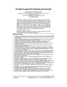
for the information we wish to extract. (These experiments were performed in a dry-air environment to eliminate the spectral absorption lines due to water vapor.19) Figure 2 displays a schematic of the interaction of the THz pulse with the sample. An incident pulse impinges on the front surface of the sample. Part of the energy is transmitted, and part is reflected. As the transmitted portion moves through the material, propagation affects the THz wave. Also, reflections can occur at internal interfaces to create multiple output pulses from a single input pulse. We capture these interactions in our model. The Fresnel equations describe the transmission and reflection of the THz wave at each interface.17 These are based on the material’s complex index of refraction in the frequency domain, ñ ( ␻ ) ⫽ n( ␻ ) ⫺ j ␬ ( ␻ ), where n( ␻ ) represents the real refractive index, ␬(␻) is proportional to the absorption coefficient, ␬ ( ␻ ) ⫽ ␣ ( ␻ )c/(2 ␻ ), and ␻ is angular frequency. The Fresnel equations at an interface between two layers are t ab 共 ␻ 兲 ⫽ r ab 共 ␻ 兲 ⫽

˜ a 共 ␻ 兲 cos ␪ 2n ñ a 共 ␻ 兲 cos ␤ ⫹ ñ b 共 ␻ 兲 cos ␪ ñ b 共 ␻ 兲 cos ␪ ⫺ ñ a 共 ␻ 兲 cos ␤ ñ a 共 ␻ 兲 cos ␤ ⫹ ñ b 共 ␻ 兲 cos ␪

,

(1)

,

(2)

where t ab ( ␻ ) is the transmission coefficient of a wave at an incidence angle ␪ from region a to region b and r ab ( ␻ ) is the reflection in region a at the a – b interface. The angle ␪ is estimated, and ␤ is an approximation of Snell’s law for nearly transparent materials (which covers all samples examined in this work)17:

␤ ⫽ arcsin

冉

n a sin ␪

冊

. (3) nb As the wave moves through a material along a ray of length d, its propagation is governed by p b 共 ␻ , d 兲 ⫽ exp

冉

⫺jn ˜ b共 ␻ 兲 ␻ d

冊

, (4) c where c is the speed of light, and the ray length is determined by d⫽

Fig. 2. Transmission and reflection pathways for a THz wave through a planar, homogenous material. We rotate the sample in the drawing to exaggerate nonnormal incidence and clarify the multiple-reflection pathways. Our model describes the interactions at each transmission or reflection interface and the propagation through the material. The resulting signal includes the first transmission through the sample and two multiples caused by internal reflections.

m ⫽ d cos共 ␪ ⫺ ␤ 兲 ,

E primary共 ␻ 兲 ⫽ E initial共 ␻ 兲 p air关 ␻ , 共 x ⫺ m 兲兴 ⫻ t 01 p sample共 ␻ , d 兲 t 10 , E first

with x the distance between the transmitter and receiver. This includes the small but measurable contribution of the refractive index from air at standard pressure and room temperature.20 We must also determine the propagation distance of the terahertz pulse in air with the sample in place. This distance between the transmitter and receiver, minus the path through the material, depends on the angle of the sample and how much the incident pulse is refracted. The amount subtracted from the distance between the emitter and the detector is defined as the following:

⫽ E initial共 ␻ 兲 p air关 ␻ , 共 x ⫺ m 兲兴

⫻ r 10 p sample共 ␻ , d 兲 t 10 ⫽ E initial共 ␻ 兲 p air关 ␻ , 共 x ⫺ m 兲兴 2 2 ⫻ t 01 p sample共 ␻ , d 兲 t 10r 10 p sample 共 ␻, d 兲,

(9) E second

(6)

multiple共 ␻ 兲

(8)

⫻ t 01 p sample共 ␻ , d 兲 r 10 p sample共 ␻ , d 兲

. (5) cos ␤ We neglect scattering (e.g., interface roughness) in our model. We consider the THz path both with and without a sample in place. For the free-air path, we have

ñ air共 ␻ 兲 ⫽ 1.00027 ⫺ j0,

(7)

As shown in Fig. 2, we examine a planar, homogeneous material placed in the pathway of the THz radiation. Owing to the Fabry–Perot effect, a number of multiples occur.15 Our iterative approach, explained in Section 3, requires that the primary and at least two multiples be present in the measured waveforms to solve for the free variables. The equations for the primary received signal and two multiples with the sample in place are

l

E ref共 ␻ 兲 ⫽ E initial共 ␻ 兲 p air共 ␻ , x 兲 ,

where ␪ ⭓ ␤ .

multiple共 ␻ 兲 ⫽ E initial共 ␻ 兲 p air关 ␻ , 共 x ⫺ m 兲兴 4 4 ⫻ t 01 p sample共 ␻ , d 兲 t 10r 10 p sample 共 ␻, d 兲.

(10) To make our system of equations more tractable, we first add Eqs. (8)–(10). This models the measured waveform that contains all three temporal signals:

(11)

Dorney et al.


We are now able to clearly discern the multiples FP( ␻ ) described by the Fabry–Perot effect. Dividing Eq. (11) by Eq. (6), we obtain ˆ 共␻兲 ⫽ H ⫽

E complete共 ␻ 兲 E ref 共 ␻ 兲 ˜ air共 ␻ 兲 ñ sample共 ␻ 兲 cos ␪ cos ␤ 4n n air共 ␻ 兲 cos ␤ ⫹ ñ sample共 ␻ 兲 cos ␪ 兴 2 关˜

冠再

⫻ exp

⫺j 关 dn ˜ sample共 ␻ 兲 ⫺ mn ˜ air共 ␻ 兲兴 ␻ c

冎冡

FP 共 ␻ 兲 . (12)

Equation (12) is essentially the same as in Duvillaret et al., but the incident angle ␪ is included.15 It provides the transfer function for our model. The complex function ñ sample( ␻ ), l, and ␪ are the only free variables (the variables d and m are dependent on l).

many global minima for any error measure. Instead, using the magnitude and unwrapped phase information provides a unique solution.15 The algorithm must unwrap the phase for both the modeled and the measured deconvolution similarly in order to make a valid comparison. In unwrapping, we require that the phase must extrapolate to zero at zero frequency. Our algorithm resets the phase at ␻ ⫽ 0 to zero and unwraps all subsequent phases, assuming that no two adjacent values have a difference greater than 2␲. We define the error by taking the absolute difference between the magnitude and the unwrapped phase of the measured data versus the model: ˆ 共 ␻ 兲兩 , mER 共 ␻ 兲 ⫽ 兩 H 共 ␻ 兲兩 ⫺兩 H ˆ 共 ␻ 兲. pER 共 ␻ 兲 ⫽ ⬔H 共 ␻ 兲 ⫺ ⬔H

In Section 2 we developed the transfer function of the ˆ ( ␻ ) models the normalized sample. Equation (12) for H interaction of the THz pulse with the material. We compare the measured signals with this model to determine the values for the free variables; however, we must first consider two signal-processing concerns, namely, data record length and regularization. The deconvolution in frequency of our measured temporal signals is H共 ␻ 兲 ⫽

E sample共 ␻ 兲 E ref 共 ␻ 兲

.

(13)

Here E sample( ␻ ) is the discrete Fourier transform (DFT) of the time-based signal with the sample in place, and E ref ( ␻ ) is the DFT of the system output without sample. Since the DFT uses circular convolution, our method requires sufficient temporal signal length to maintain the proper ordering of the features. Zero padding extends the data records obtained from the THz system. Unfortunately, this creates artificial step functions in the data where the zeros are added. To counter this effect, we taper the values to attenuate near the ends of the data record. We typically apply the taper only to the first and last 25 data points (out of 1024) to avoid modifying the THz pulses in the signal. Another consideration is the regularization of the deconvolution. Equation (13) produces good results except where very small values occur in the denominator. This introduces the need for high and low frequency limits, as seen in Fig. 1(b). The deconvolution therefore only uses the frequency information between 0.25 and 1.4 THz. Shown in Fig. 1(c) is the inverse DFT h(t) of the deconvolution H( ␻ ). It is the impulse response of the sample derived from the waveforms in Fig. 1(a). We wish to compare the deconvolution of the measured signals H( ␻ ) [Eq. (13)] with the modeled transfer funcˆ ( ␻ ) [Eq. (12)]. Unfortunately, the real and imagition H nary parts of H( ␻ ) are oscillating functions that produce

(14)

The total error over all frequencies of interest is ER ⫽

3. SIGNAL PROCESSING OF TERAHERTZ WAVEFORMS

1565

兺兩 mER 共 ␻ 兲兩 ⫹ 兩 pER 共 ␻ 兲兩 .

(15)

␻

Duvillaret et al. used a somewhat different error calculation by taking the squared error of the natural log of the magnitude and the unwrapped phase.15 Since we do not apply a parabolic-fit method to match the model to the measured signals, we do not use the same error measure. Our procedure uses a three-step process. First, we make an initial guess at the thickness. Second, our algorithm calculates the beginning functions for the complex index of refraction. The initial guess assumes a nondispersive material. Third, a gradient descent algorithm iterates the complex index of refraction function in frequency until the total error no longer decreases monotonically. Our algorithm records the final complex refractive-index function and repeats these steps for a range of thicknesses. We review each of these steps in detail below. First, the algorithm bounds the upper and lower limitsof-thickness guesses by l upper ⫽

⌬t c n 1 ⫺ n air

,

l tower ⫽

⌬t c n 2 ⫺ n air

,

(16)

where ⌬t is the time delay between the pulse in E ref(t) and the first pulse in E sample(t) of the measured signals. The parameters n 1 and n 2 limit the range of refractive indices considered. Values of n 1 ⫽ 1.2 and n 2 ⫽ 8 cover most practical cases. Second, the best initial starting function for the complex refractive index occurs when the first peak location of the temporal model’s deconvolution is the same as the first peak location of the measured deconvolution. The real refractive index and the thickness of a material control where the first peak exists in the temporal deconvolution. The imaginary index of refraction and the thickness affect the amplitude of the first peak. Assuming a nondispersive material ( flat frequency response) for the estimated n( ␻ ), the following equation governs the relationship between the thickness and the real refractive index on the basis of the location of the pulse in the measured signal’s temporal deconvolution:

1566


n⫽

再

argmax关兩 h 共 t 兲兩兴 c l

冎

⫹ 1.00027,

Dorney et al.

(17)

where l is the estimated thickness of the material selected in the first step and argmax关兩 h(t) 兩兴 is the time index of the absolute maximum of the measured temporal deconvolution. This assumes that the input signal begins at t ⫽ 0. We do not expect a constant real refractive index in most real materials, but this provides a good way to generate an initial estimate. The initial value for ␬(␻) begins at zero and increments until the absolute maximum of the modeled temporal deconvolution is less than or equal to the absolute maximum of the measured temporal deconvolution. Third, after the initialization of n( ␻ ) and ␬ (␻), they are updated by use of a gradient descent algorithm21: n new共 ␻ 兲 ⫽ n old共 ␻ 兲 ⫹ ⑀ p ER共 ␻ 兲 ,

␬ new共 ␻ 兲 ⫽ ␬ old共 ␻ 兲 ⫹ ⑀ m ER共 ␻ 兲 ,

(18)

where ⑀ is the update step size. It determines how much of an effect the magnitude and phase error has on the new values for the complex refractive index. A reasonable value is ⑀ ⫽ 0.01. The algorithm updates the complex index of refraction functions until the total error in Eq. (15) is no longer monotonically decreasing. Our algorithm applies the three steps outlined above to generate a complex index-of-refraction function for a variety of guessed thicknesses. We require a metric in order to identify which thickness and complex refractiveindex pair are the estimated properties for our sample. Total error is an obvious choice; however, a poor signalto-noise ratio (SNR) or too large a thickness stepping distance causes inaccurate results (as demonstrated below). Instead, we introduce the total variation of degree one22,23:

The total variation [Eq. (20)] is a more-robust metric than the peak-to-peak measurements of the refractiveindex functions used in previous reports.16 For a highly dispersive material, the oscillatory structure seen in Fig. 3 rides on a smoothly varying background arising from the material dispersion. In this case, the peak-to-peak measurement does not accurately characterize the amplitude of the oscillatory structure. In contrast, TV is a measure of local variations and thus provides a moreaccurate estimation of the thickness. It also tolerates noisy regions where poor regularization or noisy data induce artificial oscillations. Owing to the large range of thicknesses to be considered, we apply the three steps outlined above on three different thickness ranges and stepping distances. The first pass uses a coarse stepping distance ⌬t1 over the full range of thicknesses identified in Eq. (16). The next two passes use finer stepping distances ⌬t2 and ⌬t3 over a limited range identified from the previous pass. The deepest local minimum of the total variation on each pass determines the center point for the next-finer pass. In a limited number of simulations, the final pass did not contain a minimum; therefore we modified the total-variation metric: TV2 ⫽

兺兩D关 m 兴 ⫺ D关 m ⫹ 1 兴兩.

(21)

This modified total variation takes the absolute difference between adjacent points of Eq. (19). Using Eq. (21), we

D关 m 兴 ⫽ 兩n关 m ⫺ 1 兴 ⫺ n关 m 兴兩 ⫹ 兩␬关 m ⫺ 1 兴 ⫺ ␬关 m 兴兩, (19) TV ⫽

兺 D关m兴,

(20)

where the sum ranges over the useful data, between 250 GHz and 1.4 THz. For most samples, we do not expect that the recorded complex index of refraction will vary dramatically from one frequency sample to the next, since the sampled frequency step size is relatively small. (Our temporal window width is approximately 60 ps with a sample rate of 7 fs, which gives a frequency sampling of ⌬f ⬵ 17 GHz.) Though the index may have strong variations with frequency, the majority of solid materials do not have spectral features that are sharp compared with ⌬f.3,24 Note that this method fails for samples with sharp spectral features (e.g., gases). We use the recorded complex index of refraction to calculate the total variation at each thickness. As shown in Fig. 3, the final complex index of refraction shows a marked reduction in oscillations at the proper thickness. We observe, however, that the amount of ripple in n( ␻ ) and ␬(␻) also decreases as l increases. By identifying the thickness at which the deepest local minimum for total variation occurs, our algorithm identifies the proper thickness.

Fig. 3. Final real index of refraction obtained from our algorithm at various guessed thicknesses for a sample of GaAs. As we approach the appropriate thickness, the oscillations in the complex index of refraction decrease. The general trend as the guessed thickness increases, however, is the decrease in amplitude for the complex refractive index. This leads us to use the deepest local minimum and the total variation of degree of one metric in Eqs. (19)–(21).

Dorney et al.


1567

are able to amplify the variations in the smoothness measure. Use of the modified total variation on only the final pass produced a local minimum for all experimental and simulated results.

4. RESULTS We examine several materials through both simulation and experimental data and investigate the general limits of this method. The simulated results are for materials with a low real refractive index, since the number of multiples in experimental data is SNR limited. The THz system provides data for several high-index materials. We present data for Si, GaAs, InP, and LiNbO3 (ordinary axis) using TV and TV2 metrics. We first consider the data for a silicon wafer sample. Previous THz-TDS studies used silicon as a sample material since it has essentially zero absorption and a flat spectral response [i.e., ñ ( ␻ ) ⫽ 3.42 ⫺ j0].15,16,24 Figure 4(a) shows the total error plotted over the initial coarse sampling of thicknesses for a high-resistivity silicon wafer sample ( ␳ ⬎ 104 ⍀ cm). Note that the error curve initially has an exponentially decaying trend at small-tomedium thicknesses with a large portion of the error terms near zero. The beginning exponential shape in Fig. 4(a) results from the exponential dependence of the transfer function on ñ sample( ␻ ). The argument of the exponential function in Eq. (12) must remain constant as l (the variables d and m are dependent on l) linearly increases; therefore, while l is relatively small, ñ sample( ␻ ) must remain relatively large. Consequently, the algorithm cannot reduce the error below some limit. Conversely, as l becomes relatively large, ñ sample( ␻ ) decreases, and the error decreases greatly during the gradient descent. In effect, our total error curve is mapped onto an exponentially decaying function. A global minimum may exist at the correct thickness; however, signal noise may prevent its existence, or the thickness step size ⌬t 1 may step over the global minimum. We therefore locate the deepest local minimum. Note that the total-error measure is lower in Fig. 4(b) than in Fig. 4(a), demonstrating the effect of ⌬t 1 being coarser than ⌬t 2 . In Fig. 4(b) we show the total-variation measure after the minimum total error at a particular thickness is achieved. The resulting curve is again exponentially decreasing. An inconsistent dip, however, in the TV curve occurs at the proper thickness because of a good match between the model and measured signals. The inclusion of the Fabry–Perot effect in Eq. (12) causes the inconsistent dip in the total-error curve at 0.49 mm. The model matches the measured deconvolution better at this location relative to the adjacent thicknesses. The deepest local minimum identifies the proper thickness. The totalvariation metric has an advantage over total error in that the concave function around the local minimum occurs over a wider range of guessed thicknesses; therefore the selection of ⌬t 1 is less critical for total variation. Figure 4(c) shows the estimated real and imaginary indices of refraction at the thickness identified from the TV2 metric. Repeated measurements made with calipers give a thickness of 0.51 ⫾ 0.02 mm. The results of the

Fig. 4. (a) Total error between the model and measured signals, according to Eq. (15), for a 0.51 ⫾ 0.02-mm-thick sample of silicon plotted over a wide range of thicknesses. The box indicates the boundaries for the next graph. (b) We compare the total error curve (circles) against the total variation metric (triangles) for the intermediate stepping distance 0.01 mm. The deepest local minimum for total variation provides a better indicator of the actual thickness than total error since it has a wider concave region and is more noise tolerant. The measured thickness with error region is shown. (c) Corresponding real and imaginary indices of refraction for the thickness identified by the modified totalvariation deepest local minimum of the final pass (solid lines). Literature data puts the complex index of refraction of silicon at 3.42 ⫺ j0 (dashed lines).

estimation agree with the caliper measurements, within the uncertainty. The solid lines indicate the estimated values. The dashed lines are the values for the complex refractive index taken from the literature.24 The estimated and the expected values are essentially superimposed, and both the real and the imaginary estimated values are independent of frequency as expected. Since the primary source of error is sample alignment, we included the incidence angle ␪ in our model. For other samples, silicon is used as a reference material to determine the THz beam angle. We adjust the value of ␪ in the model until the known optical parameters of silicon are obtained. The angle is then fixed for all other samples. A second sample is high-resistivity, semi-insulating GaAs, which has a somewhat higher refractive index.

1568


Figure 5(a) shows the total variation over a range of thicknesses by way of the same procedure as for silicon outlined above. The estimated thickness for GaAs is 0.63 mm, compared with the measured thicknesses of 0.65 ⫾ 0.02 mm. The initial stepping distance used to identify a local minimum was 0.1 mm. In Fig. 5(b), we show the complex index of refraction at the estimated thickness. The data points represent the literature values,25 with a dashed line to guide the eye. Again, good agreement is obtained. In particular, the small dispersion of the real part of the index is estimated correctly. Next we examine InP. The same plots are generated in Fig. 6 as in the GaAs experiment. Note the absence of a local minimum for total error as compared with total variation in Fig. 6(a) with a 0.1-mm stepping distance used for ⌬t 1 . Obviously, ⌬t 1 must be reasonably small to identify the local minimum. The complex index of refraction for InP is shown in Fig. 6(b). We note that the three samples, Si, GaAs, and InP, all have similar indices of refraction. Nonetheless, we are able to distinguish clearly between these materials, and also to extract the thickness of each sample accurately. A similar analysis for LiNbO3 (ordinary axis) is shown in Fig. 7. The estimated thickness is 0.49 mm, and the measured thickness is 0.50 ⫾ 0.02 mm. The real index of refraction tracks the literature data well; however, some low-frequency noise existed in the raw signals.25 The increasing absorption of LiNbO3 at higher frequencies is captured by our estimate. Since the technique requires that the primary and two multiples be present in the measured waveforms, it is difficult to obtain the parameters from materials with low indices of refraction. To explore this limit, we turn to

Fig. 5. (a) Total-variation measure for GaAs shown with a 0.1-mm stepping distance. (b) Complex refractive index for the estimated thickness (solid line) compared with the index from the literature (dashed line). We note the slight dispersion of the material.

Dorney et al.

Fig. 6. (a) Total error and total-variation measure for InP shown with a 0.1-mm stepping distance. We note that the initial stepping distance did not produce a local minimum for total error, although one does exist for total variation. (b) Real refractive index for the estimated thickness compared with the literature data. Literature data is not available for the imaginary refractive index over the frequency range shown, but an imaginary value of 8.7 ⫻ 10⫺3 at 6 THz is reported in the literature.25

simulation to validate our approach. For low real refractive indices, we create a simulation to produce both the input and the output time-domain waveforms. A Rayleigh distribution models the faster current rise and slower current fall in a photoconductive switch. We modify the distribution to smooth the region around the origin so that it is differentiable. The derivative of a modified Rayleigh distribution is used as the model for a single-cycle THz pulse. We simulate a material with a constant complex index of refraction n ˜ sample( ␻ ) ⫽ 1.9 ⫺ j0 and l ⫽ 1.27 mm. The algorithm described above produced the total error and total variation curves shown in Fig. 8(a). The deepest local minimum for total error does not occur at the correct thickness with a 0.1-mm stepping size for thickness. As a result, we introduced the total variation of degree one in Eqs. (19) and (20) as shown in Fig. 8(a). Figure 8(b) shows both the total error and the total variation curves with a 0.001-mm thickness stepping size. Here, the global minimum coincides with the thickness of the simulated material and with the deepest local minimum of the total variation metric in Fig. 8(a). To obtain the global minimum, a very small step size is required owing to the narrow width of the minimum in Fig. 8(b). The computational load therefore is extremely high, and a correct global minimum was not always observed with real data owing to the addition of noise. We also note that the false local minimum in the total error at an approximate thickness of 2 mm does not appear at all in the total-

Dorney et al.

variation curves. The modified total-variation metric [Eq. (21)] has been used in the final pass to analyze all of the data in Figs. 4–7, 9. The total-variation measure has several advantageous features. First, it selects the local minimum on the basis of oscillations in the complex refractive index; however, it measures local oscillations as opposed to a global peak-topeak measure. Dispersive materials, noisy raw-data signals, and nonuniform oscillations in the estimated ñ sample( ␻ ) are better characterized by a local measure. Second, total variation ignores the multiple local minima in the total error measure as shown in Figs. 8(a) and 8(b). Third, a wider concave region exists around the actual thickness, as compared with the total error measure. Finally, if the initial guessed thickness is greater than the actual thickness and subsequent thickness guesses only increase, the total variation will not report a local minimum. The natural conclusion would be to start with a lower guessed thickness or check the thickness stepping distance. Last, we examine the limitations of the total-variation method. To be mathematically tractable, the primary and two multiples must occur in the signal with the sample. As the real index of refraction decreases, the amplitude of the multiples decreases owing to the reduced internal reflections. For a given SNR ratio, there is a corresponding limit to the minimum real refractive index that can be studied. From SNR measurements of the THz system, we reasonably expect a ratio of 1500 between the peak-to-peak waveform amplitude and the rms. noise amplitude.4 Using simulations and a captured noise signature, we determine the minimum real index resolved by our algorithm. Figure 9 shows the range of parameters for which the method is applicable. The circles denote test cases that passed with the thicknesses indicated by the vertical dashed lines and a nondispersive, real index of refraction. The darker shaded area represents the region where the test cases passed. Below this region the method is lim-


1569

Fig. 8. (a) Total error (circles) and total variation (triangles) for a simulated material with a low real index of refraction. The deepest local minimum for total error does not occur at the proper thickness with a 0.1-mm-thickness stepping size. (b) Total error and total variation as in (a) with a 0.001-mm-thickness stepping size. A global minimum is possible for both measures, but real data often provide only a deepest local minimum, owing to noise. Total variation is a more robust and computationally efficient metric to indicate the correct material thickness, owing to the larger thickness step size allowed.

Fig. 9. Limits of our method displayed for a simulated material at a signal-to-noise ratio of 1500:1. The circles indicate the test cases that passed for the thickness indicated by the vertical dashed lines. At each point, the real refractive index was constant across frequency, while the imaginary component was zero. The darker area represents the passing region. The area below the passing region is signal-to-noise limited. The lighter area at the top indicates a region that should pass; however, the initial stepping distance for thickness needs to be smaller and/or the data record needs to be longer. At larger thicknesses, the multiple reflections might exceed the data record length.

Fig. 7. Complex index of refraction for LiNbO3 (ordinary axis) displayed at the estimated thickness of 0.49 mm. The real refractive index tracks the literature data well; however, some lowfrequency noise exists in the raw-data signals. We note the increasing absorption at higher frequencies captured by our estimate, as expected.

ited by SNR. Above this region we expected the simulations to pass. The initial step size, however, was too large to produce a local minimum, or the analysis window size (25 ps in this simulation) limited the number of multiples. Obviously, both the thickness stepping size and the analysis window can be changed depending on the material under investigation. For example, in Fig. 6(a) a

1570


Dorney et al.

reduced thickness stepping size would be advantageous. Consequently, our method is applicable in both of the shaded regions in Fig. 9.

Boyd and Jon Johnson to maintain and automate the laboratory and thank T. Rabson for the loan of a LiNbO3 crystal.

5. CONCLUSIONS

Corresponding author Daniel Mittleman can be reached at the address on the title page; by phone, 713348-5452; by fax, 713-348-5686; or by e-mail, [email protected].

We have introduced a method to simultaneously calculate the thickness and complex index of refraction of an unknown homogenous sample with use of THz time-domain spectroscopy (THz-TDS). The THz-TDS system provides a noncontact, nondestructive approach for investigation. Also, analysis can occur on samples enclosed in standard packaging materials (e.g., cardboard, cellophane, styrofoam), since these materials are transparent at low THz frequencies. Our method simply requires the primary transmission and two multiples in the output waveform. Our method uses a model-based approach that minimizes the absolute difference between measured waveforms and the model by use of a gradient descent algorithm. For each thickness over a range of thicknesses, we use the final iteratively determined complex index of refraction to calculate the total-variation measure. The total-variation metric determines the smoothness of the estimated complex index of refraction. The deepest local total variation minimum provides an estimate at each pass. By scanning smaller intervals on each of three passes, we refine the search over thickness. The final pass uses the smallest thickness range with the smallest stepping distance. We apply the modified total-variation metric on the final pass. The total-variation metric exploits the fact that most materials have a smoothly varying spectrum. Our metric measures the local oscillatory artifacts, as in Fig. 3, which can characterize dispersive materials, noisy raw-data signals, and nonuniform oscillations in the estimated complex refractive index. This is more general than minimizing the peak-to-peak amplitude, as in Ref. 16. Also, a null result is reported if the scanned thickness range does not overlap the actual thickness. Our algorithm operates on a single signal pair (reference and signal with sample) for each experiment (with the potential inclusion of a reference-material waveform to determine the angle of incidence); however, sample translation allows for pixel-by-pixel imaging. The addition of simple optics provides a method to achieve a diffraction-limited focal spot approximately 250 ␮m in diameter.5 Efforts to determine similar parameters, but at a lower real index of refraction, are ongoing. The ability to parameterize materials with multiple interfaces or with composite construction is also of interest. Outlines of the algorithms used for this work are available at www.dsp.rice.edu/⬃mit.

REFERENCES 1. 2. 3.

4. 5. 6. 7. 8. 9. 10. 11. 12.

13. 14. 15.

16.

17.

ACKNOWLEDGMENTS We acknowledge support for this work by the Army Research Office, the Environmental Protection Agency’s National Center for Environmental Research and Quality Association, the National Science Foundation, the Office of Naval Research, and the Defense Advanced Research Projects Agency. We also acknowledge the efforts of Joel

18. 19. 20.

P. R. Smith, D. H. Auston, and M. C. Nuss, ‘‘Subpicosecond photoconducting dipole antennas,’’ IEEE J. Quantum Electron. 24, 255–260 (1988). M. van Exter and D. Grischkowsky, ‘‘Characterization of an optoelectronic terahertz beam system,’’ IEEE Trans. Microwave Theory Tech. 38, 1684–1691 (1990). M. C. Nuss and J. Orenstein, ‘‘Terahertz time-domain spectroscopy (THz-TDS),’’ in Millimeter and Submillimeter Wave Spectroscopy of Solids, G. Gru¨ner, ed. (Springer– Verlag, Heidelberg, Germany, 1998), and references therein. D. M. Mittleman, R. H. Jacobsen, and M. C. Nuss, ‘‘T-ray imaging,’’ IEEE J. Sel. Top. Quantum Electron. 2, 679–692 (1996). B. B. Hu and M. C. Nuss, ‘‘Imaging with terahertz waves,’’ Opt. Lett. 20, 1716–1718 (1995). D. M. Mittleman, S. Hunsche, L. Boivin, and M. C. Nuss, ‘‘T-ray tomography,’’ Opt. Lett. 22, 904–906 (1997). D. M. Mittleman, M. Gupta, R. Neelamani, R. G. Baraniuk, J. V. Rudd, and M. Koch, ‘‘Recent advances in terahertz imaging,’’ Appl. Phys. B 68, 1085–1094 (1999). Q. Wu, F. G. Sun, P. Campbell, and X.-C. Zhang, ‘‘Dynamic range of an electro-optic field sensor and its imaging applications,’’ Appl. Phys. Lett. 68, 3224–3226 (1996). Z. G. Lu, P. Campbell, and X.-C. Zhang, ‘‘Free-space electrooptic sampling with a high-repetition-rate regenerative amplified laser,’’ Appl. Phys. Lett. 71, 593–595 (1997). D. M. Mittleman, R. H. Jacobsen, R. Neelamani, R. G. Baraniuk, and M. C. Nuss, ‘‘Gas sensing using terahertz timedomain spectroscopy,’’ Appl. Phys. B 67, 379–390 (1998). L. Hui, F. Zhongyu, and Y. Jianqi, ‘‘Infrared imaging solar spectrograph at Purple Mountain Observatory,’’ Sol. Phys. 185, 69–76 (1999). K. Sato, T. Sato, H. Sone, and T. Takagi, ‘‘Development of a high-speed time-resolved spectroscope and its application to analysis of time-varying optical spectra,’’ IEEE Trans. Instrum. Meas. IM-36, 1045–1049 (1987). R. E. Burge, X.-C. Yuan, J. N. Knauer, M. T. Browne, and P. Charalambous, ‘‘Scanning soft X-ray imaging at 10 nm resolution,’’ Ultramicroscopy 69, 259–278 (1997). D. Colton and R. Kress, Inverse Acoustic and Electromagnetic Scattering Theory, 2nd ed. (Springer–Verlag, Heidelberg, Germany, 1998), pp. 2–7. L. Duvillaret, F. Garet, and J. Coutaz, ‘‘A reliable method for extraction of material parameters in terahertz timedomain spectroscopy,’’ IEEE J. Sel. Top. Quantum Electron. 2, 739–746 (1996). L. Duvillaret, F. Garet, and J. Coutaz, ‘‘Highly precise determination of both optical constants and sample thickness in teraherz time-domain spectroscopy,’’ Appl. Opt. 38, 409– 415 (1999). E. Hecht, Optics, 2nd ed. (Addison–Wesley, Reading, Mass., 1987). M. Dobrin and C. Savit, Introduction to Geophysical Prospecting, 4th ed. (McGraw-Hill, New York, 1988). M. van Exter, C. Fattinger, and D. Grischkowsky, ‘‘Terahertz time-domain spectroscopy of water vapor,’’ Opt. Lett. 14, 1128 (1989). P. E. Ciddar, ‘‘Refractive index of air: new equations for the visible and near infrared,’’ Appl. Opt. 35, 1566–1573 (1996).

Dorney et al. 21. 22.

S. Haykin, Adaptive Filter Theory (Prentice-Hall, Englewood Cliffs, N.J., 1996). J. E. Odegard and C. S. Burrus, ‘‘Discrete finite variation: a new measure of smoothness for the design of wavelet basis,’’ in Proceedings of the International Conference on Acoustics, Speech, and Signal Processing (Institute of Electrical and Electronics Engineers, New York, 1996), pp. 1467–1470.

Vol. 18, No. 7 / July 2001 / J. Opt. Soc. Am. A 23. 24.

25.

1571

F. Jones, Lebesgue Integration on Euclidean Space (Jones and Bartlett, Boston, Mass., 1993). D. Grischkowsky, S. Keiding, M. van Exter, and C. Fattinger, ‘‘Far-infrared time-domain spectroscopy with terahertz beams of dielectrics and semiconductors,’’ J. Opt. Soc. Am. B 7, 2006–2015 (1990). E. D. Palik, Handbook of Optical Constants of Solids (Academic, San Diego, Calif., 1985).