Material Point Method Calculations with Explicit ... - University of Utah

c 2003 Tech Science Press Copyright

CMES, vol.4, no.6, pp.649-663, 2003

Material Point Method Calculations with Explicit Cracks J. A. NAIRN1

Abstract: A new algorithm is described which extends the material point method (MPM) to allow explicit cracks within the model material. Conventional MPM enforces velocity and displacement continuity through its background grid. This approach is incompatible with cracks which are displacement and velocity discontinuities. By allowing multiple velocity fields at special nodes near cracks, the new method (called CRAMP) can model cracks. The results provide an “exact” MPM analysis for cracks. Comparison to finite element analysis and to experiments show it gets good results for crack problems. The intersection of crack surfaces is prevented by implementing a crack contact scheme. Crack contact can be modeled using stick or sliding with friction. All results are two dimensional, but the methods can be extended to three dimensional problems. keyword: Material point method, cracks, fracture, numerical methods, contact 1

Introduction

The material point method (MPM) has recently been developed as a numerical method for solving problems in dynamic solid mechanics [Sulsky, Chen, and Schreyer (1994), Sulsky, Zhou, and Schreyer (1995), Sulsky and Schreyer (1996), Zhou (1998)]. In MPM, a solid body is discretized into a collection of points much like a computer image is represented by pixels. As the dynamic analysis proceeds, the solution is tracked on the material points by updating all required properties such as position, velocity, acceleration, stress state, etc.. At each time step, the particle information is extrapolated to a background grid which serves as a calculational tool to solve the equations of motions. Once the equations are solved, the grid-based solution is used to update all particle properties. This combination of Lagrangian and Eulerian methods has proven useful for solving solid me-

chanics problems including those with large deformations or rotations and involving materials with history dependent properties such as plasticity or viscoelasticity effects [Sulsky, Chen, and Schreyer (1994), Sulsky, Zhou, and Schreyer (1995), Sulsky and Schreyer (1996), Zhou (1998)]. MPM is amendable to parallel computation [Parker (2002)], implicit integration methods [Guilkey and Weiss (2002)], and alternative interpolation schemes that improve accuracy [Bardenhagen and Kober (2003)]. Although MPM uses a background grid and is frequently compared to finite element methods, a new derivation or MPM [Bardenhagen and Kober (2003)] presents it as a Petrov-Galerkin method that has similarities with meshless methods such as Element-Free Galerkin (EFG) methods [Belytschko, Lu, and Gu (1994)] and MeshlessLocal Petrov-Galerkin (MLPG) methods [Atluri and Shen (2002a), Atluri and Shen (2002b), Atluri and Zhu (1998)]. The “meshless” aspect of MPM, despite the use of a grid, derives from the fact that the body and the solution are described on the particles while the grid is used solely for calculations. The body can translate through the grid. Furthermore the grid can be discarded each time step and redrawn which makes MPM suitable to adaptive mesh methods. It is essential for any extension to MPM, such as presented here, to preserve the separation between the grid and the particles. MPM, EFG, and MLPG differ in their methods used to derive shape functions and in their selection of test functions during numerical implementation [Bardenhagen and Kober (2003), Atluri and Shen (2002a)].

One potential application of MPM is as a tool in dynamic fracture modeling. It was recently shown that MPM can accurately calculate fracture parameters such as energy release rate [Tan and Nairn (2002)], but those results were for a crack at a symmetry plane and thus the crack could be described by symmetry conditions alone. Conventional MPM is not capable of handling explicit, internal cracks. The problem is that conventional MPM meth1 Material Science and Engineering, University of Utah, Salt Lake ods extrapolate particle information to a single velocity City, Utah 84112, USA

650

c 2003 Tech Science Press Copyright

field on the background grid. A property of the background grid, which is analogous to finite element analysis grids, is that all displacements in the single velocity field are continuous. Because representation of cracks requires displacement discontinuities, MPM can not represent cracks. This paper describes a modified material point method labeled as CRAMP for ”CRAcks” with ”Material Points.” The following list gives the essential differences between CRAMP and conventional MPM:

CMES, vol.4, no.6, pp.649-663, 2003

calculations for existing, internal cracks. The subject of evaluating fracture parameters at crack tips and predicting crack propagation will be in future work. The crack description used, however, is very flexible. It is a trivial matter to extend the crack during a dynamic analysis once the harder problem of deciding when and where to extend the crack has been solved. Finally, the CRAMP algorithm is efficient. Comparison between conventional MPM and CRAMP show the crack calculations to be only about 10% slower. The most time consuming part of the CRAMP algorithm is determining which particles interpolate to which velocity field at each node.

1. Cracks are described in 2D as a series of line segments. The end-points of the line segments can be additional mass-less particles to make it easy to add 2 MPM With Explicit Cracks — CRAMP crack descriptions to standard MPM data structures. This section describes the CRAMP algorithm for includ2. Each node in the background grid is allowed to have ing explicit cracks in MPM calculations. The features of multiple velocity fields. If the node is far from any the algorithm are given here; the full algorithm is procrack, the node will have a single velocity field as vided in the Appendix. The first task is to describe the in conventional MPM. For nodes near a crack, how- internal cracks. One simple way to introduce displaceever, each node will have separate velocity fields for ment discontinuities into MPM would be to introduce information interpolated from particles on opposite cracks in the background grid. Although this approach sides of a crack. can handle certain problems, it severely limits the flexibility of MPM. The background grid is supposed to serve 3. Most calculations in the MPM algorithm needed to as a calculational tool and not as a device to carry inforbe adjusted to account for the possibility that a parmation about the solution or about the solid. It would ticular node might have multiple velocity fields. also be difficult or impossible to translate the crack along 4. When nodes have separate velocity fields and dis- with the body during large deformation calculations. In placement continuities, it is possible for the two CRAMP, the crack is instead described as a series of line sides of the crack to cross over each other. To pre- segments. For compatibility with MPM data structures, vent non-physical crossing, all calculations at nodes the endpoints of the line segments are massless material with multiple velocity fields must implement con- points. By translating the crack segments along with the tact methods. The algorithm in this paper can model solution, it is possible to track cracks in moving bodies. A problem can contain any number of cracks. crack contact by stick or by sliding with friction. 5. A modified scheme for updating stresses and strains was added which appears to improve energy calculations. An important application of crack calculations is to do fracture predictions. Because fracture work requires accurate energy calculations, it was important to optimize the MPM energy results. This last correction can be applied to conventional MPM as well as to CRAMP.

2.1

Multiple Velocity Fields

The influence of cracks on the MPM solution is that they influence the velocity fields at some nodes in the background grid. In conventional MPM, the first step in the algorithm is to extrapolate the particle momenta and masses to the background grid. The equations are [Sulsky, Zhou, and Schreyer (1995)]: np

np

k k All results in this paper are for 2D calculations. In most pki = ∑ m p vkp Si,p mDk (1) i = ∑ m p Si,p cases, the extension to 3D is simple and obvious. The one p=1 p=1 exception is the crack description. In 3D, the crack needs to be described by connected surfaces instead of line seg- where pki is nodal momentum, vkp is particle velocity, m p k is the shape function for node i evalments. The algorithm presented here does stress analysis is particle mass, Si,p

651

MPM Calculations with Explicit Cracks

uated at the current position of particle p, and mDk is i the nodal mass in the lumped (or diagonal) mass matrix. The superscript k indicates these terms apply to the kth MPM step. In this approach, each nodal point has a single momentum and displacement discontinuities are not allowed. To allow displacement discontinuities, CRAMP allows each node to have three types of velocity fields one for particles on the same side of all cracks as the node (0), one for particles above a crack relative to the node (1), and one for particles below a crack relative to the node (2). The first step in crack calculations is thus to examine each particle-node combination (with non-zero shape function) and determine the appropriate velocity field denoted by

momenta become 0

pki, j = pki, j + ∆t fi,totj

j = 0, 1, 2 (as needed)

(5)

where ∆t is the time step. When updating particle positions, velocities, stresses, and strains, the equations only use the velocity field appropriate to each particle/node pair. For example, updating of position becomes xk+1 p

=

xkp + ∆t

0

nn

k pki,ν(p,i) Si,p

i=1

mDk i,ν(p,i)

∑

(6)

Above are some examples of the modified equations; all the required modifications are detailed in the Appendix.

If the body is translating, all cracks need to translate (2) along with it. This task is accomplished by calculating the center of mass velocity of each node with multiple This determination is done by a line-crossing algorithm. velocity fields: First, a line is drawn from particle p to node i. If the 00 line does not cross any crack, the velocity field is 0; if it ∑3j=1 pki, j ϕi, j k vi,cm = 3 (7) crosses a crack from above, the velocity field is 1; if it ∑ j=1 mDk i, j ϕi, j crosses a crack from below, the velocity field is 2. The field determination is the most time consuming part of where ϕi, j is 1 or 0 depending on whether or not velocCRAMP and must be done efficiently; an efficient algo- ity field j is present at node i. Once all nodal velocities rithm is given in the Appendix. Once the velocity field’s are reduced to a single field, the mass-less particles that are determined, the modified, initial MPM extrapolations define the crack can move using standard MPM methods become for updating particle position.  np  k 2.2 Crack Surface Contact pki, j = ∑ m p vkp Si,p δ j,ν(p,i)    ν(p, i) = 0, 1, or 2

p=1 np

j = 0, 1, 2

(3) Several times during each MPM step, the nodal momenta and velocities are updated. These updates may occur as a p=1 consequence of boundary conditions or when implementEach node may have one to three velocity fields denoted ing the equations of motion. Whenever the nodal momenta change, it is essential to verify that the change corby index j on pki, j and mDk i, j . Each velocity field interpolates only from particles contributing to that field as responds to a physically allowed change which is defined determined by the Kronecker delta function δ j,ν(p,i) . Al- here as meaning that opposite sides of cracks do not cross though three velocity fields are defined, no node should over each other. To prevent non-physical changes, the ever have more that two velocity fields — one each for CRAMP algorithm includes contact methods. The methods are based on the contact methods develop by Bardenparticles on the two sides of a crack. hagen [Bardenhagen, Brackbill, and Sulsky (2000), BarThe possible existence of multiple velocity fields carries denhagen, Guilkey, Roessig, Brackbill, Witzel, and Fosthrough the remainder of the algorithm. Each conventer (2001)], but there are two key differences. First, the tional MPM calculation must consider all velocity fields. methods in Bardenhagen, Brackbill, and Sulsky (2000) For example, the total nodal forces (with damping) are and Bardenhagen, Guilkey, Roessig, Brackbill, Witzel, tot int ext k fi, j = fi, j + fi, j − κpi, j j = 0, 1, 2 (as needed) (4) and Foster (2001) were for contact between dissimilar materials; here contact is within the same material but on where fi,intj and fi,extj are internal and external forces at a two sides of a crack. Second, their methods used to idennode and κ is a damping coefficient. The updated nodal tify contact did not work well for internal cracks; they mDk = i, j

k δ j,ν(p,i) ∑ m p Si,p

   

652

c 2003 Tech Science Press Copyright

CMES, vol.4, no.6, pp.649-663, 2003

would either identify contact too soon or identify it un- the angle between the relative velocities and the crack reliably. This section describes the contact methods in surface normal, the cracks are assumed to be separated if CRAMP. they are moving apart as defined by The identification of crack surface contact is based (vki,a − vki,b ) · nˆ ≤ 0 (12) mostly on nodal volume at crack nodes (i.e., nodes with multiple velocity fields). The total nodal volume (which where nˆ is the crack surface normal. If the crack surfaces is a nodal area in 2D calculations) is calculated during are moving towards each other, the cracks are assumed to be in contact and the momenta are adjusted. The crack each MPM step using surface normal can be calculated earlier in the algorithm np k k k Vi = ∑ Vp Si,p (8) during the line-crossing algorithm. Whenever a line from a particle to a node crosses a crack, the normal to that p=1 crack segment is saved for that node. The normal at a where Vpk is the volume of particle p or an area in 2D given node is the average of all such normal vectors. The calculations defined by normal is defined as directed from above the crack to below the crack. mp Vpk = (1 + εkp,xx )(1 + εkp,yy ) (9) Once contact is identified (by Vrel > Vcontact or by crack ρ pt p surfaces moving towards each other), the momenta are where ρ p and t p are the density and thickness of the 2D adjusted by two alternate methods. The simplest contact particle. Whenever momenta change, the nodal volumes method is contact by stick conditions. The stick method at all nodes with multiple velocity fields are normalized simply reverts to conventional MPM where the momenta by the undeformed volume. For regular grids the un- above and below the crack are set equal to each other deformed volume is the volume of each element in the and equal to the center-of-mass momenta. The required background grid; for irregular grids, the undeformed vol- momenta changes to implement stick conditions are ume includes a portion of each element containing that k Dk k mDk node. The relative volume is defined as i,a pi,b − mi,b pi,a ∆pki,a = ∆pki,b = −∆pki,a (13) Dk + mDk m k i,a i,b Vi Vrel = unde f (10) These changes conserve total momentum. Vi Two critical relative volumes are preselected as Vsep (less than 1) and Vcontact (greater than 1). If Vrel < Vsep , the crack surfaces are assumed to be separated and no changes in momenta are needed. If Vrel > Vcontact , the cracks surfaces are assumed to be in contact and momenta are adjusted as explained below. The region Vsep < Vrel < Vcontact is a gray area and a second method is used to decide whether or not contact is present.

A frictional sliding contact method follows the approach of Bardenhagen, Guilkey, Roessig, Brackbill, Witzel, and Foster (2001). In physical terms, this method adjusts the velocity above the crack to be
v˜ ki,a = vki,a − ∆vn nˆ + µ0 ˆt (14)

where ˆt is a unit normal tangential to the crack surface in the direction of sliding and µ0 is an effective coefficient of friction defined by Several second methods are possible, but the calculations   ∆vt here used relative velocity of the two crack surfaces [Bar0 µ = min µ, (15) ∆vn denhagen, Brackbill, and Sulsky (2000), Bardenhagen, Guilkey, Roessig, Brackbill, Witzel, and Foster (2001)]. Here µ is the actual coefficient of friction, and ∆v and n Once a crack node with Vsep < Vrel < Vcontact is found, the ∆v are the components of the relative crack face velocit velocities above and below the crack are calculated from ties normal and tangential to the crack: vki,a =

pki,a mDk i,a

vki,b =

pki,b mDk i,b

(11)



∆vn = vki,a − vki,b · nˆ ∆vt = vki,a − vki,b · ˆt

(16)

When µ0 reduces to ∆vt /∆vn , the surfaces are sticking due where a and b indicate the velocity fields corresponding to friction or the velocities are adjusted to equal the cento particles above and below the crack. By examining ter of mass velocities. When µ0 reduces to µ, the contact

653

MPM Calculations with Explicit Cracks

is by friction. In the limit of frictionless sliding (µ = 0), µ0 is always zero, the crack surface velocities normal to the surfaces are adjusted to be equal and the tangential velocities remain unchanged. All CRAMP algorithm steps are in terms of nodal momenta instead of velocities. The above velocity equations in terms of momenta correspond to adjusting the momenta above and below the crack by " ! # Dk k Dk k
m p − m p i,a i,b i,b i,a ∆pki,a = · nˆ nˆ − µ0 ˆt Dk Dk mi,a + mi,b k k ∆pi,b = −∆pi,a (17) ˆ where t is now a unit vector tangential to the crack surface that is in the same direction as the crack line segments and µ0 is a signed quantity given by  ∆vt   −µ if < −µ   ∆vn   ∆vt µ0 = (18) +µ if > +µ  ∆vn   ∆vt    otherwise ∆vn Finally, the normal and tangential velocity components can be calculated from ∆vn = ∆vt

=

k Dk k mDk i,a pi,b − mi,a pi,b · nˆ mDk i,a k Dk k mDk i,a pi,b − mi,a pi,b ˆ ·t mDk i,a

(19)

were examined and slightly revised from previous methods in the literature [Sulsky, Chen, and Schreyer (1994), Sulsky, Zhou, and Schreyer (1995), Sulsky and Schreyer (1996), Zhou (1998), Bardenhagen (2002)]. As explained in the appendix, updating the stresses and strains on the particles involves calculating the strain increment for the current step and then using a constitutive law to determine the stress increment. The strain increment is a function of the current strain rate which is calculated from the current nodal velocities (see Subtask 2 for updating stresses and strains in the Appendix). There are several alternatives for which nodal velocities to use for the updating process. In an early MPM paper [Sulsky, Chen, and Schreyer (1994)], the nodal velocities were calculated after updating the nodal momenta. This approach, referred to as the “Update Stress Last” or USL, has serious numerical difficulties which are revealed by considering a node which interacts with only a single particle. Following through the algorithm in the Appendix, the nodal velocity used for strain rates would at such a node would be

vi =

vkp + ∆t

−

σkp · Gki,p k Si,p

f pk + bp + mp

! (20)

For simplicity, this analysis only considers a single velocity field and ignores damping. Only a single velocity field is considered, because only one is possible when there is only a single particle. As a consequence, all discussion in this section applies to both conventional MPM and to CRAMP. The first term in the brackets causes a problem. When the one particle is on the opposite side of k ) will the element from the node, the shape function (Si,p approach zero, but its gradient (Gki,p ) will not. The first term is thus unstable.

One difference between this frictional contact method and the one in Bardenhagen, Guilkey, Roessig, Brackbill, Witzel, and Foster (2001) is that the same normal is used for both crack surfaces (it is defined from the crack line segments) and thus momentum is exactly conserved. In Bardenhagen, Guilkey, Roessig, Brackbill, Witzel, and Foster (2001), the two contacting materials had separate There are two solutions to the USL dilemma. The first sonormal vectors and momentum was only conserved when lution was given by Sulsky, Zhou, and Schreyer (1995). those normals were equal and opposite. Their approach was to adopt a momentum based algorithm similar to the approach in the Appendix. It was 2.3 Modified Method to Update Particle Stresses and not the use of momentum that improved the algorithm, Strains but rather the way nodal velocities were calculated before One part of each MPM step involves updating the parti- updating particle stresses and strains. In their approach, cle stresses and strains. If this task is not done optimally, referred to as “Modified Update Stress Last” or MUSL, there can be numerical difficulties and inaccuracies in en- the updated particle momenta are extrapolated to the grid ergy calculations. Because accurate energy results are a second time before calculating the nodal velocities (see essential for fracture calculations, the updating methods Task 6c in the appendix). Tracing a node with a single

654

c 2003 Tech Science Press Copyright

CMES, vol.4, no.6, pp.649-663, 2003

particle, the nodal velocities used for strain rates become nn

k fitot Si,p

i=1

mDk i

vi = vkp + ∆t ∑

(21)

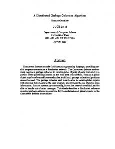
Although some nodal masses in the denominator (mDk i ) may approach zero, whenever the mass is close the zero, k identically close to zero there will be a corresponding Si,p to cancel it out. This approach greatly improves the stability of MPM. An alternate fix is to update strains before updating momentum [Bardenhagen (2002)]. In this approach, referred to as “Update Stress First” or USF, the nodal velocities (for a single-particle node) used for Figure 1 : CRAMP analysis (top) and conventional strain rates are simply MPM analysis (bottom) of an end-loaded double canvi = vkp (22) tilever beam. The colors indicate magnitude of the tensile stress in the x direction (blue compression to red tension). which clearly have no numerical difficulties. The material had properties E = 0.1 MPa, ν = 0.33, and MUSL and USF are nearly identical. MUSL finds ve- ρ = 1.5 g/cm3 . The full specimen was 100×36×1 ( in locities for momenta extrapolated at the end of an MPM mm); the crack length was 50 mm. The end loads were step while USF finds velocities from the same momenta 0.4 mN. by extrapolating at the beginning of the next time step. The only mathematical difference between these two approaches is the shape functions used in the extrapolation. k while USF uses Sk+1 . In numerous cal- simulation was continued until the stress stabilized. The MUSL using Si,p i,p culations, both give greatly improved energy calculations numerical details are given in the figure caption. As excompared to USL methods. MUSL tends to slowly dissi- pected, the crack opens, there are tensile bending stresses pate energy while USF tends to slowly increase in energy on the inner surfaces of the DCB arms and compression [Bardenhagen (2002)]. This observation leads to an ob- stresses on the outer surfaces. vious compromise which combines MUSL and USF by Although the above DCB calculation was a full calcuupdating stresses and strains both before updating nodal lation with an explicit crack, the same problem can be momenta and after updating (and re-extrapolating) nodal solved by symmetry without the need to model explicit momenta. In this approach, referred to as “Update Stress cracks. The method is to analyze half the specimen and Averaged” or USAVG, the strain increment at each up- to fix the grid points on the left half of the lower edge of dating is divided by 2 to use the two methods equally. In the specimen to have zero y-direction displacement (or numerous calculations, MPM results using USAVG con- zero y-direction velocity) throughout the analysis. The serves energy nearly exactly. Sample calculations com- results, given in the bottom of Fig. 1, show that a symparing USAVG to USL, MUSL, and USF are given in the metry analysis gives numerically identical results to the next section. full analysis, thus confirming the crack algorithm correctly accounts for the presence of a crack. Of course, 3 Results and Discussion this result was a goal of CRAMP — to develop an algorithm that gives the “exact” MPM result in the presence 3.1 Opening Crack in Double Cantilever Beam of cracks. Here “exact” means that the MPM calculaThe top of Fig. 1 shows the results of a CRAMP calcula- tions for the top half of the full specimen are exactly the tion on a double cantilever beam specimen (DCB) with a same as the calculations done when considering only half crack half way through the specimen at the mid-plane. the specimen (bottom of Fig. 1). Similarly, the calculaThe sample was end-loaded at time zero and damped tions in the bottom half of the full specimen are exactly to have the results converge to the static solution. The the same as calculations that would be used in analysis

655

MPM Calculations with Explicit Cracks

An alternate approach to handling explicit cracks in MPM is to modify the calculations using node-visibility criteria. In node-visibility methods, a line is drawn from each particle to each node. If that line crosses a crack, than that node no longer influences the calculations for that particle. Node visibility [Belytschko, Lu, and Gu (1994)] and the related diffraction criteria [Organ, Fleming, and Belytschko (1996)] have been the most common choices for implementing cracks in EFG [Belytschko and Tabbara (1996)] and MLPG [Ching and Batra (2001), Batra and Batra (2002)] methods. Although node visibility can also implement cracks in MPM, it leads to less accurate results than the CRAMP method. The above definition of “exact” MPM could be rephrased as a “crack patch” test in which the results of any crack algorithm applied to a symmetric problem with an explicit crack are compared to a standard analysis with no crack algorithm that includes the crack by symmetry conditions alone. An algorithm passes the test if the results of the two analysis are numerically identical. The CRAMP method passes the “crack patch” test while MPM with node visibility does not. Similarly, because node visibility and diffraction criteria in EFG and MLPG modify the shape functions differently than when the crack is defined only by symmetry conditions, those methods also would not pass a “crack patch” test. For an additional check, the MPM results were compared to static finite element analysis results (FEA). The FEA analysis used the same grid of rectangular, 4-noded elements that was used for the MPM calculations. Figure 2 plots the x direction stress along the mid-plane of the specimen. To find the MPM stresses at the mid-plane, the particle stresses were extrapolated to the grid by the same methods used to extrapolate momenta to the grid. The FEA and MPM results are very close. Although 4node elements are not ideal for bending problems and the element size was large, the results show the accuracy of MPM to be similar to that of FEA and provide further evidence that CRAMP is getting the correct solution in the presence of cracks.

0.0010 FEA

0.0008 Stress (MPa)

of a lower-half specimen. The complication in a full specimen is that both halves need to use the mid-plane nodes for normal MPM calculations. This simultaneous use of the mid-plane nodes is accomplished naturally in the CRAMP algorithm by those nodes having two velocity fields.

MPM

0.0006 0.0004 0.0002 0.0000 0

20

40

60

80

100

Distance (mm)

Figure 2 : Comparison of FEA results to CRAMP results. The plot is for σxx as a function of position along the mid-plane of the specimen. The peak stress is at the crack tip. The material properties are given in the caption of Fig. 1

3.2

Cracks Experiencing Contact

The DCB analysis was for an opening crack. The results in this section give a simulation when crack contact is important. The simulation is for two disks moving towards each other, contacting, and then bouncing apart. The disk on the left has a horizontal crack in the middle of the disk. The length of the crack is equal to one third the diameter of the disk. The disk on the right has the same size crack but oriented in the vertical direction. When the disks first make contact, the axial compression of the disk on the left causes mode I loading of the crack and the crack opens [Shetty, Rosenfield, and Duckworth (1987)]. The transverse compression to the disk on the right causes the cracks faces to contact and the contact algorithm keeps the surfaces from crossing. After the impact event, the two disks begin to vibrate and the cracks open and close. The contact algorithm keeps the solution proceeding correctly. The plots in Fig. 3 show four snapshots of the solution. The cracks are indicated by a black line and the colors for the material points indicate tensile stress in the y direction. Frame a shows the initial conditions with closed cracks and zero stress; the disks have initial velocities towards each other. Frame b shows a moment soon after contact. The diametrical compression has opened the crack in the left disk and red zones show crack tip stress concentrations in the y-direction normal stress. The crack

656

c 2003 Tech Science Press Copyright

CMES, vol.4, no.6, pp.649-663, 2003

on the right has closed and the contact algorithm kept the surfaces from crossing each other. In frame c, the disk vibrations have caused the crack on the left to close and the contact algorithm prevents cross over. The crack on the right has opened slightly. By frame d, the crack on the left has opened again.

a. 0 ms

b. 20 ms

c. 32 ms

d. 45 ms

Figure 3 : Four snapshots for two disks with cracks colliding and separating. The colors indicate y direction tensile stress (blue minimum to red maximum) The material properties were E = 0.1 MPa, ν = 0.33, and ρ = 1.5 g/cm3 . The disks were 30 mm in diameter and 1 mm thick. The cracks were centrally located and 10 mm long. The crack surfaces were frictionless. At the beginning the disks were moving towards each other, each with a speed of 1000 mm/sec.

The contact algorithm handles crack surface contact well, but it was essential to implement the volume method to determine contact rather than rely on other methods such as relative velocity [Bardenhagen, Guilkey, Roessig, Brackbill, Witzel, and Foster (2001)] or normal traction methods [Bardenhagen, Brackbill, and Sulsky (2000)]. When other contact methods were used, the crack surfaces would think they were in contact long before visual evidence indicated there were actually in contact. For example, the contact between the two disks is handled by conventional MPM. In conventional MPM, two particles will interact (i.e., be in contact) whenever they both interact with a particular node. The contact space between the disks in frame B is a typical example of MPM contact where the closest approach is determined by the mesh density. When analyzing internal cracks, it is important to have new contact methods that allow closer approach before numerical contact. The volumetric scheme used here worked well for allowing realistic contact. The critical volumes used for these soft disks were Vsep = 0.9 and Vcontact = 1.1. These critical values can work for any materials, but stiffer materials might be handled more efficiently and more accurately by using critical values closer to one. The volumetric method is robust for internal cracks, but has deficiencies for edge cracks. When there are edge cracks, the relative volume at a node might be less then one even when the cracks are in contact. The above algorithm might mistakenly consider such cracks as separated. The problem is that the undeformed volume is calculated from the element area while the true undeformed volume should account for the node being near the edge of a material. This problem did not affect the above edgecrack DCB results because the cracks were always separated. To better handle edge cracks in contact, enhanced volumetric methods are needed. One approximate approach is to normalize the nodal volume to the total number of particles interacting with that node. This approach improves the contact detection at edge nodes, but sometimes gives invalid contact detection at internal nodes. This problem will be the subject of future work.

MPM Calculations with Explicit Cracks

3.3

657

Comparison to Experiment

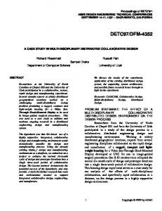
This example considers a much larger problem (58017 material points), stiffer materials, and comparison to experiments. The configuration, illustrated in Fig. 4 shows five transparent disks (poly methylmethacylate (PMMA)) constrained by a jig to remain planar and aligned. At time zero, the left side is impacted (at 6 m/sec) and high speed photography was used to record photoelastic fringes [Roessig and Foster (2001), Roessig (2001)]. To study crack effects, the central disk contained a crack aligned with the loading direction having a length equal to half the diameter of the disk. The top half of Fig. 4 shows experimental results for one particular time. The stress concentrations at the crack tip are evident by the increased number of fringes. The front of the stress wave has just reached the last disk.

Figure 4 : Five poly methylmethacylate disks impact loaded from the left side. the central disk has a crack parallel to the loading direction of length equal to half the diameter of the disk. The top figure gives the experiment birefringence pattern at one particular time. The The MPM simulations modeled the five disks by an ap- bottom figure gives the calculated birefringence pattern. proach similar to that described in Bardenhagen, Guilkey, Roessig, Brackbill, Witzel, and Foster (2001). The disk material was set to a high modulus material (E = 174860, the CRAMP code is correctly modeling the presence of ν = .214, ρ = 1.90). A high modulus material was used the crack. instead of actual PMMA modulus because the analysis One might think that this problem is symmetric along involved less total displacement. The simulations and the mid-plane or that the analysis could be done by conexperiments were compared by normalizing to the wave sidering half the sample with fixed displacements along speeds in the different materials [Bardenhagen, Guilkey, the mid-plane except for no constraints on the crack surRoessig, Brackbill, Witzel, and Foster (2001)]. Simu- face. Examination of the full results, however, reveals lations with lower moduli that had larger displacements the the crack surfaces experience contact as the stress developed noise in regions where particles crossed el- waves pass by the crack. It was thus necessary to do a ement boundaries. The methods in Bardenhagen and full analysis and use the crack contact methods to handle Kober (2003) can solve some or all of such noise issues, contact. An analysis of half the specimen develops nonbut those methods were not available in the CRAMP physical crack surface displacements as the crack surface code. The impactor was modeled as a material with much displacements extend past the mid-plane. higher density (E = 17486, ν = 0.214, ρ = 190) to emulate the impact event. The photoelasticity fringes were 3.4 Energy Calculations calculated by taking a periodic function of the principle The final example is not a crack problem, but an examstress difference. The equation used was ination of the energy results using the four methods for  q  updating stresses - USL, MUSL, USF, and USAVG. The
2 cos k f σxx − σyy +4τ2xy (23) problem, illustrated in Fig. 5, is for transverse impact on a polymer specimen. The simulation mimics experwhere k f is physically a fringe constant for the material. imental results in Nairn (1989). The beam (of dimenBy comparison to experiments, k f was determined to be sions 88×6×12.95 mm with span of 68 mm) was Delrin 0.0889 (for stresses in MPa). There were 30 elements polyoxymethylene polymer (E = 2900 MPa, ν = 0.33, or 60 material points across the diameter of each disk. ρ = 1.5). The impactor was given a modulus 10 times The simulation results in the bottom of Fig. 4 are for the higher, a higher density, and a thickness chosen to have simulation time closest to the experimental time. The its’ total mass match the experimental impact mass of predicted fringes agree well with experimental results. In 367 g. The impact velocity was set to the experimental particular the fringe patterns around the crack show that result of 2.43 m/sec. No gravity was used and thus the

658

c 2003 Tech Science Press Copyright

CMES, vol.4, no.6, pp.649-663, 2003

sum of kinetic and strain energy should remain constant throughout the simulation. Figure 6 shows total energy in the MPM simulation using each of the four stress updating methods. By tracking the kinetic energy in the impactor, the beam impact started at about 0.4 ms and continued until about 4.2 ms. The original MPM method, or USL, gave poor results. The simulation had to be stopped at about 3.6 ms because it became unstable and one of the material points left the grid. The three other methods gave stable results and better energy results. The MUSL approach slowly dissipated energy (with two step drops) while the USF approach slowly increased in energy (with two step increases). These observations are similar to results by these two methods in Bardenhagen (2002). The USAVG approach conserved energy. The total energy remained within ±0.18% of the average throughout the entire simulation. By the algorithm, USAVG is an average of the USF and MUSL methods, but it does not lead to results that are simple average of the other methods. For example, because USF increased in energy more than MUSL decreased in the energy, their average increased in energy with time. The USAVG result, however, did not follow this average but rather gave nearly exact conservation of energy. Similar comparisons between USF, MUSL and USAVG were found in numerous other MPM results.

Figure 5 : Initial configuration and material point discretization for transverse impact of a disk on a polymer beam. The dimensions and material properties are given in text of the paper. The colors indicate beam material (red), impactor material (blue), and beam support material (green).

1.30

Algorithm Efficiency

Profiling of the CRAMP code showed that most additions due to crack effects add very little overhead to MPM code. The one exception is the need to examine particlenode pairs to determine the appropriate velocity field. This step involves determining whether or not a line from a particle to a node crosses a crack. It is important to implement this step as efficiently as possible. The Appendix gives one algorithm that works well. There are two key components. First, the line crossing algorithm should be efficient. Second, great improvement is possible by screening particle-node pairs and skipping the check entirely for those that can not cross a crack. A simple way to do this screening, which led to an order of magnitude efficiency increase in this step, is to keep track of the extent of each crack or the minimum and maximum x and y values for all end points of the segments of the crack. Then, when checking any particle node pair, the line crossing code can be skipped whenever the rectangle defined by the particle and node points has no in-

1.20 Total Energy (J)

3.5

USF USAVG

1.10

MUSL 1.00 USL 0.90 0

1

2

3

4

5

6

Time (ms)

Figure 6 : Total energy (kinetic + strain energy) during impact of a disk on a polymer beam (see Fig. 5) by MPM using four different methods for updating stress and strain in each time step — USL (red), MUSL (black), USF (blue), and USAVG (green). The methods are explained in the text of the paper.

MPM Calculations with Explicit Cracks

tersection with the extent of the crack. With optimal linecrossing algorithm combined with screening using crack extents, the fracture calculations in this paper averaged only 10% longer than the comparable MPM calculation with no cracks. 4

Conclusions

This paper describes a CRAMP algorithm which extends MPM to naturally handle explicit cracks. When the fracture code is written efficiently, especially the new line crossing section, the CRAMP code achieves crack calculations with very letter extra cost in calculation time. The results show that CRAMP gets the correct MPM solutions and comparisons to both FEA and experiments show that it gets good results for crack problems. To account for crack surface contact, there are checks for contact and both stick and sliding with friction can be handled. The method to detect crack contact is robust for internal cracks but may need some adjustment for problems involving edge cracks. Crack propagation is easily handled by simply moving the crack or adding crack segments at any time step. The important problem that remains is the calculation of crack tip or fracture parameters followed by prediction of crack propagation. This problem will be the subject of future work. Although this paper describes a 2D algorithm, extension to 3D is possible. In 3D, the crack line needs to be replaced by a crack surface described by planar elements instead line segments. The line crossing algorithm needs to be replaced by a 3D area crossing algorithm.

659 Atluri, S. N.; Zhu, T. (1998): A New Meshless Local Petrov-Galerkin (MLPG) Approach in Computational Mechanics. Computational Mechanics, vol. 22, pp. 117–127. Bardenhagen, S. G. (2002): Energy Conservation Error in the Material Point Method. J. Comp. Phys., vol. 180, pp. 383–403. Bardenhagen, S. G.; Brackbill, J. U.; Sulsky, D. (2000): The Material Point Method for Granular Materials. Computer Methods in Applied Mechanics and Engineering, vol. 187, pp. 529–541. Bardenhagen, S. G.; Guilkey, J. E.; Roessig, K. M.; Brackbill, J. U.; Witzel, W. M.; Foster, J. C. (2001): An Improved Contact Algorithm for the Material Point Method and Application to Stress Propagation in Granular Material. Computer Modeling in Engineering & Sciences, vol. 2, pp. 509–522. Bardenhagen, S. G.; Kober, E. M. (2003): The Generalized Interpolation Material Point Method. in press, 2003. Batra, R. C.; Batra, H.-K. (2002): Analysis of Elastodynamic Deformations Near a Crack/Notch Tip by the Meshless Local Petrov-Galerkin (MLPG) Method. Computer Modeling in Engineering & Sciences, vol. 3, pp. 717–730.

Belytschko, T.; Lu, Y. Y.; Gu, L. (1994): Element-Free Acknowledgement: This work was support by a grant Galerkin Methods. Int. J. Num. Meth. Engrg., vol. 37, from the Department of Energy DE-FG03-02ER45914 pp. 229–256. and by the University of Utah Center for the Simulation Belytschko, T.; Tabbara, M. (1996): Dynamic Fracof Accidental Fires and Explosions (C-SAFE), funded by ture Using Element-Free Galerkin Methods. Int. J. Nuthe Department of Energy, Lawrence Livermore National mer. Methods in Eng., vol. 39, pp. 923–938. Laboratory, under Subcontract B341493. Ching, H.-K.; Batra, R. C. (2001): Determination of Crack Tip Fields in Linear Elastostatics by the MeshAtluri, S. N.; Shen, S. (2002): The Meshless Lo- less Local Petrov-Galerkin (MLPG) Method. Computer cal Petrov-Galerkin (MLPG) method: A Simple & Less- Modeling in Engineering & Sciences, vol. 2, pp. 273– Costly Alternative to the Finite Element and Boundary 289. Element Methods. Computer Modeling in Engineering Guilkey, J. E.; Weiss, J. A. (2002): Implicit Time & Sciences, vol. 3, pp. 11–52. Integration for the Material Point Method: Quantitative Atluri, S. N.; Shen, S. P. (2002): The Meshless Local and Algorithmic comparisons with the Finite Element Petrov-Galerkin (MLPG) Method. Tech. Science Press. Method. in press, 2002. References

660

c 2003 Tech Science Press Copyright

CMES, vol.4, no.6, pp.649-663, 2003

Nairn, J. A. (1989): The Measurement of Polymer Appendix A: CRAMP Algorithm Viscoelastic Response During an Impact Experiment. This appendix summarizes the CRAMP algorithm to inPolym. Eng. & Sci., vol. 29, pp. 654–661. clude explicit cracks and some revisions to MPM to update stresses and strains by a method that minimizes disOrgan, D. J.; Fleming, M.; Belytschko, T. (1996): sipation of energy. The algorithm is for 2D calculations, Continuous Meshless Approximations for Nonconvex but most vector results translate easily into a 3D algoBodies by Diffraction and Transparency. Computational rithm. In the following, subscript p always refers to Mechanics, vol. 18, pp. 225–235. a particle property, subscript i always refers to a nodal property, bold face refers to a vector or a tensor, plain Parker, S. G. (2002): A Component-based Artext refers to a scalar, and an over bar indicates a spechitecture for Parallel Multi-Physics PDE Simulation. cific quantity (actual quantity divided by particle denIn International Conference on Computational Science sity). The following single algorithm includes four op(ICCS2002) Workshop on PDE Software. tions for updating particle stresses and strains denoted as USL, MUSL, USF, and USAVG; these methods were deRoessig, K. M. (2001): 2001. Personal communication. scribed in the text of the paper. Roessig, K. M.; Foster, J. C. (2001): Experimen- Task 0: At the beginning of the (k + 1)th MPM analysis tal Simulations of Dynamic Stress Bridging in Plastic step, all information for the numerical solution resides Bonded Explosives. in press, 2001. on the particles. The information relevant to the follow algorithm are particle position (xkp ), velocity (vkp ), Shetty, D. K.; Rosenfield, A. R.; Duckworth, W. H. specific stress (σkp ), strain (εkp ), mass (m p ), density (ρ p ), (1987): Mixed-Mode Fracture in Biaxial Stress State: thickness (t p for 2D calculations), and any other mateApplication of the Diametral-Compression (Brazilian rial properties needed for constitutive law calculations. Disk) Test. Eng. Fract. Mech., vol. 26, pp. 825–839. The shape functions and shape function gradients are defined from the current particle positions as Sulsky, D.; Chen, Z.; Schreyer, H. L. (1994): A Park ticle Method for History-Dependent Materials. Comput. Si,p = Ni (xkp ) and Gki,p = ∇Ni (xkp ) (24) Methods Appl. Mech. Engrg., vol. 118, pp. 179–186. where Ni (x) are the basic element shape functions. In Sulsky, D.; Schreyer, H. K. (1996): Axisymnmetric practice, the shape functions and their gradients are not Form of the Material Point Method with Applications to calculated and stored (which would require a large arUpsetting and Taylor Impact Problems. Comput. Meth- ray), but anytime they are calculated during the algorithm, they refer to the particle position at the beginning ods. Appl. Mech. Engrg, vol. 139, pp. 409–429. of the (k + 1)th step. The particle volume, which is an Sulsky, D.; Zhou, S.-J.; Schreyer, H. L. (1995): Appli- area in 2D calculations, is found from cation of a Particle-in-Cell Method to Solid Mechanics. mp Vpk = (1 + εkp,xx )(1 + εkp,yy ) (25) Comput. Phys. Commun., vol. 87, pp. 236–252. ρ pt p Tan, H.; Nairn, J. A. (2002): Hierarchical Adaptive Task 1: Loop over the particles. For each particle, draw Material Point Method in Dynamic Energy Release Rate a line from that particle to each node in the element conCalculations. Comput. Meths. Appl. Mech. Engrg., vol. taining that particle and use a line-crossing algorithm to 191, pp. 2095–2109. calculate ν(p, i) = 0, 1, or 2 which determines the velocity field for particle p at node i. An optimized lineZhou, S.-J. (1998): The Numerical Prediction of Ma- crossing algorithm is given below. Field 0 means the terial Failure Based on the Material Point Method. PhD drawn line does not cross a crack; field 1 means the line thesis, Department of Mechanical Engineering, Univer- crosses a crack and the particle is above the crack relasity of New Mexico, 1998. tive to the node; field 2 means the line crosses a crack

661

MPM Calculations with Explicit Cracks

and the particle is below the crack relative to the node. y directions, set the total forces for all velocity fields at If ν(p, i) = 1 or 2 and node i does not have that ve- that node to zero to prevent acceleration in the next task. locity field, then allocate a new velocity field for that Task 4: Update nodal point momenta node. Only nodes near cracks will have multiple veloc0 ity fields and except in unusual conditions, no node will j = 0, 1, 2 (29) pki, j = pki, j + ∆t fi,totj ever have more than two velocity fields — one for particles on one side of the crack and one for particles on Adjust any momenta for crack contact effects by the procedure listed below. the other side. In the same loop, calculate nodal momenta and lumped Task 5: Loop over the particles to update particle position and velocity using Sulsky, Zhou, and Schreyer masses for all needed velocity fields using (1995): np

k δ j,ν(p,i) ∑ m p vkp Si,p

pki, j =

p=1 np

mDk i, j

∑

=

j = 0, 1, 2

xk+1 p

(26) k m p Si,p δ j,ν(p,i)

j = 0, 1, 2 vk+1 p

p=1

where δi,ν(p,i) is the Kronecker delta function. For use in the contact algorithm, calculate total nodal volumes using np

Vik =

k ∑ Vpk Si,p

(27)

p=1

Task 2: Apply any boundary conditions to nodal momenta calculated in the previous task and check for crack contact by the procedure listed below. For USF or USAVG methods only, update particle stresses and strains by the procedure listed below. The new particle 0 0 stresses and strains are denoted σkp and εkp . For USL and MUSL methods, the stresses and strains are not up0 0 dated and thus set σkp = σkp and εkp = εkp . Task 3: Loop over the particles again. For each particle calculate internal, external, and total forces for all velocity fields in use. The equations [Sulsky, Chen, and Schreyer (1994), Sulsky, Zhou, and Schreyer (1995)] now adjusted for multiple velocity fields are (each for j = 0, 1, 2): np

fi,intj =

∑



 0 k −m p σkp · Gki,p + m p bp Si,p δ j,ν(p,i)

p=1 np

fi,extj =

k δ j,ν(p,i) ∑ f pk Si,p

=

(28)

p=1

fi,totj = fi,intj + fi,extj − κpki, j where bp are any specific body forces on a particle, such as gravity, f pk are forces applied directly to particles, and κ is a damping constant which can be used to damp the analysis. If any nodes have fixed displacement in x or

=

xkp + ∆t vkp + ∆t

0

nn

k pki,ν(p,i) Si,p

i=1 nn

mDk i,ν(p,i) tot k fi,ν(p,i) Si,p

i=1

mDk i,ν(p,i)

∑

∑

(30)

Notice that the momentum, force, and mass used is this update come from the specific velocity field for each particle/node pair determined by the line crossing results for ν(p, i) evaluated in Task 1. Task 6: a. For USL method only, update particle stresses and strains as described below to find σk+1 and p 00 0 k+1 k k ε p and set pi, j = pi, j for later use. b. For USF only, the stress and strain update was done 0 0 = σkp , εk+1 = εkp . Also set before and thus set σk+1 p p 00 0 pki, j = pki, j for later use. c. For MUSL or USAVG only, extrapolate the new particle velocities to the grid to get a revised set of nodal momenta using: 00

pki, j =

np

k ∑ m p vk+1 p Si,p δ j,ν(p,i)

j = 0, 1, 2

(31)

p=1

Adjust any momenta for crack contact effects by the procedure listed below. Note that this extrapolation uses the new particle velocities but the shape functions and line crossing results from the original particle positions. This approach was found to give better results than one using updated information. Update particle stresses and strains using the new nodal momenta by the procedure and εk+1 listed below to find σk+1 p p . Task 7: Calculate center of mass velocity for each node with multiple velocity fields: 00

vki,cm

=

∑3j=1 pki, j ϕi, j ∑3j=1 mDk i, j ϕi, j

(32)

662

c 2003 Tech Science Press Copyright

where ϕi, j = 1 if there exists a p such that δ j,ν(p,i) = 1, otherwise ϕi, j = 0. In other words, ϕi, j is 1 or 0 depending on whether or not velocity field j is present for node i. Use this nodal velocity field to update the positions of all line segments that define the cracks by standard position updating methods. Task 8: All information is now on the particles and if needed the cracks have translated. All nodal and mesh information can be discarded and then return to Task 0 to begin the next MPM calculation step.

CMES, vol.4, no.6, pp.649-663, 2003

first case is the most common; the other three correspond to the node being on the crack segment, on the start point of the crack segment, or on the end point of the crack segment, respectively. The cases where the material point is on the crack segment can be ignored. Similarly, the particle is below the crack if the signs are (+ − −+), (+ − −0), (0 − −0), or (+0 − 0). All other combinations of signs indicate the line does not cross the line segment. In practice, many signed area calculations can be skipped. For example is the signs of (123) and (123) are (++), there is no need to evaluate the signs of (341) and (342) because the line can not cross the segment. Subtask 4: One complication is that a given xp to xn line might cross more than one segment in a single crack. In this situation, the crossing is ignored unless there are an odd number of crossings. To include this possibility, the previous two steps must check all segments in a crack before deciding if there is a crossing, but if Subtask 1 finds no intersection, the check for all segments in that crack can be skipped.

Line Crossing Algorithm: The most time consuming, new calculation required for CRAMP is the linecrossing calculation in Task 2. It is important for this calculation to be optimal and precise. The only numerical difficulty occurs when a node lies very close to the crack path. In some line-crossing algorithms, numerical round off in this situation could result in two particles on the same side of the crack being labeled as being on opposite sides. The complementary problem of when a material point lines very close to a crack path never occurs because the contact methods keep particles from Contact Algorithm: Any time the nodal momenta are reaching the crack path. calculated (i.e., in Tasks 2, 4, and 6c), the above alA line-crossing algorithm in 2D based on signed ar- gorithm must check cracks for contact. If contact is eas of certain triangles solved the problem of nodes on found, adjust nodal momenta for all velocity fields at cracks. For any three points, x1 , x2 , and x3 , the signed nodes experiencing contact. If any momenta change in Task 4, back calculate the corresponding total nodal area of the triangle with those vertexes is given by forces to match the new momenta. This recalculation is Area = x1 (y2 − y3 ) + x2 (y3 − y1 ) + x3 (y1 − y2 ) (33) needed to insure particle velocities update correctly in Task 5. The algorithms for deciding on contact and for This area is positive if the path from x1 to x3 is counter adjusting momenta are given in the MPM With Explicit clockwise, negative if it is clockwise, and zero if the Cracks section. points are collinear. Using this signed area, the algoUpdating Stresses and Strains: Because the above alrithm is as follows: gorithm includes four different methods for updating Subtask 1: Before doing any calculations, determine stresses and strains (USL, MUSL, USF, and USAVG), if the rectangle defined by the particle (x1 = xp ) and it includes several locations for the updates (Tasks 2, 6a, the node (x2 = xn ) under consideration intersects the and 6c). All stress and strain updates use the following extent of the segment endpoints in the crack. If it does procedure: not, the line does not cross the crack and rest of the Subtask 1: Calculate nodal point velocities using the algorithm can be skipped for that crack. current nodal point momenta Subtask 2: For each crack segment with endpoints x3 pk∗ i, j and x4 , calculate the sign of the areas of triangles vi, j = Dk∗ j = 0, 1, 2 (as needed) (34) mi, j (123), (124), (341), and (342) denoted as “+”, “−” or “0”. where k∗ means the most recently calculated momenta Subtask 3: The particle is above the crack if the signs are (− + +−), (− + +0), (0 + +0), or (−0 + 0). The

and vi, j is only calculated for active velocity fields (ϕi, j = 1).

663

MPM Calculations with Explicit Cracks

Subtask 2: Loop over particles and find the strain increment for the current step from ∆εkp

∇vkp + ∇vkp = ∆t 2

T

∗

(35)

In two dimensions, the velocity gradient at the material points involves four terms calculated from the outer products nn

∇vkp = ∑ vi,ν(p,i) ⊗ Gki,p

(36)

i=1

Here ∆t ∗ is the time step for USL, MUSL, and USF, but half the time step for USAVG. Notice that USAVG updates stresses and strains twice during each step (in Tasks 2 and 6c); each update gives half the update for the current step. Subtask 3: Input the strain increment (∆εkp , and the individual components of the velocity gradient, ∇v p , if needed) into a material constitutive law and update the particle stresses. Any constitutive law may be used.