Hindawi Discrete Dynamics in Nature and Society Volume 2017, Article ID 4730253, 13 pages https://doi.org/10.1155/2017/4730253
Research Article Mathematical Model and Algorithm for the Reefer Mechanic Scheduling Problem at Seaports Jiantong Zhang and Yujian Song School of Economics & Management, Tongji University, Shanghai 200092, China Correspondence should be addressed to Yujian Song;
[email protected] Received 11 October 2016; Accepted 14 February 2017; Published 6 March 2017 Academic Editor: J. R. Torregrosa Copyright © 2017 Jiantong Zhang and Yujian Song. This is an open access article distributed under the Creative Commons Attribution License, which permits unrestricted use, distribution, and reproduction in any medium, provided the original work is properly cited. With the development of seaborne logistics, the international trade of goods transported in refrigerated containers is growing fast. Refrigerated containers, also known as reefers, are used in transportation of temperature sensitive cargo, such as perishable fruits. This trend brings new challenges to terminal managers, that is, how to efficiently arrange mechanics to plug and unplug power for the reefers (i.e., tasks) at yards. This work investigates the reefer mechanics scheduling problem at container ports. To minimize the sum of the total tardiness of all tasks and the total working distance of all mechanics, we formulate a mathematical model. For the resolution of this problem, we propose a DE algorithm which is combined with efficient heuristics, local search strategies, and parameter adaption scheme. The proposed algorithm is tested and validated through numerical experiments. Computational results demonstrate the effectiveness and efficiency of the proposed algorithm.
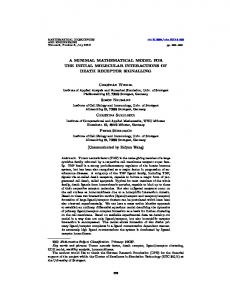
1. Introduction In today’s globalized world, cost-effective transportation systems that link global supply chains are the engine fuelling economic development and prosperity. With 80 percent of global merchandise trade by volume carried by sea and handled by ports worldwide, the strategic economic importance of maritime transport as a trade enabler cannot be overemphasized. World container port throughput surpassed 600 million 20-foot equivalent units in 2012, increased by an estimated 3.8 percent (UNCTAD 2013). Among container businesses, to export perishable goods, such as beefs and fruits, refrigerated containers or reefers (see Figure 1) are employed to maintain customers’ goods with the best quality during the transport to final destinations. With this trend, some companies, like CMA CGM, have investigated in large fleets of reefers. NUCTAD (2013) also mentions that Container Industry San Antonio is going to be the first reefer container factory in South America. The company is scheduled to produce 40,000 reefer containers per year. South America is among the regions with the highest demand for empty reefer containers for export. The impact on society of reefers is vast, allowing consumers all
over the world to enjoy fresh produce at any time of year and experience previously unavailable fresh produce from many other parts of the world (https://en.wikipedia.org). As for container terminals, this trend brings new challenges to managers: (i) a large amount of reefers is transshipped at a relatively short time; (ii) the accurate arrival and departure time of reefers are not known beforehand. To guarantee the service quality for reefers, without increasing the cost of employing reefer mechanics, the terminal managers need to optimize the usage of current employees. Since the late 1990s, researchers mainly focus on optimization of equipment resource, such as quay cranes scheduling [1–3], yard transfer vehicle routing [4], berth allocation [5], stowage planning [6], yard crane scheduling [7], and yard block allocation [8]. A large number of literatures can be found in excellent surveys [9–11]. However, rare effort has been put on optimization of human resource, such as reefer mechanics here. To guarantee the quality of goods transported in reefers, port managers need to properly arrange mechanics to plug in power when the reefers arrive and unplug power from the nearest electricity pole where reefer is stored. Such tasks need to be performed properly, since later completion may affect the
2
Discrete Dynamics in Nature and Society
2. Problem Description
Figure 1: Fleet, reefers, and mechanics (http://www.cma-cgm.com & http://photos.oregonlive.com).
quality of cargos, which cannot be recovered. The problem described is similar to the scenario of parallel machine total tardiness minimization scheduling where jobs arrive over time. Liu et al. [12], Chu [13], Yalaoui and Chu [14], and Kacem et al. [15] investigate parallel machine scheduling problem with setup times and devise a branch and bound algorithm to solve it. Schutten and Leussink [16] discuss parallel machine scheduling problem with release times where due dates and setup times are also in consideration and present a branch and bound algorithm to solve this problem. Chen and Lee [17] implement a column generation approach for parallel machine scheduling problem with a due window. These approaches can obtain optimal results but are applicable to problems with a limited number of jobs and machines, due to an unacceptable computation time. Hence, heuristic algorithms prevail against exact algorithms in this field. Chiang et al. [18] propose a memetic algorithm. Torabi et al. [19] formulate it as biobjective problem and construct a PSO algorithm to solve it. Lamothe et al. [20] propose an efficient simulated annealing algorithm for it. The only literature referring to reefer mechanic scheduling problem (RMSP) can be found in [21, 22]. A general model that consists of the scheduling of straddle carriers, automated guided vehicles, stacking cranes, and the reefer mechanics is developed by Hartmann [21]. A genetic algorithm is applied to solve it. Quite recently, Hartmann [22] studies the RMSP and attempts to minimize the total distances between any two consecutive jobs due to their different locations. An insertion-based heuristic is proposed and evaluated through a simulation model. However, there is no reference related to such a scheduling problem in the domain of deterministic scheduling literature. To the best of our knowledge, we are the first to study reefer mechanic scheduling problem in the view of optimization aspect. The main contributions which distinguish our work from theirs are (i) development of a mathematical model for RMSP, (ii) design of an efficient differential evolutionary algorithm (DE), and (iii) extensive numerical experiments to verify its superiority. The remainder is organized as follows. In Section 2, we describe the problem and establish the MIP (Mixed Integer Programming) model. A DE algorithm is developed in Section 3. Section 4 presents extensive computational results. Section 5 concludes the work.
2.1. Background. Some restricted stacking areas on the yard are equipped with electricity poles for supporting reefers. Reefer mechanics plug the arriving container and unplug the departing container not later than a desired handling completion time. Each task of plugging or unplugging takes a certain time. After completion of one task, a mechanic walks to the location of next task. As mentioned in Hartmann (2013), the basic process associated with reefer handling is as follows: (i) the terminal operating system (TOS) transmits job information to a reefer mechanic, (ii) the reefer mechanic receives the job on his portable radio data device, (iii) the mechanic walks to the reefer location, and (iv) the mechanic performs the plugging or unplugging of the container and returns to (i). Each plugging job is related to an arrival reefer and each unplugging job corresponds to a departing container. Each of the jobs has a release time, that is, the earliest possible start time of handling, a processing time, that is, the time taken for the unplugging/plugging and the repair of mechanical problems, and a due date, that is, the desired completion time of handling. The release time of a plugging job corresponds to the time when a container is placed at yard by a stacking crane. Considering unplugging jobs, the release time depends on the allowed time without power. The due date indicates the time at which the stacking crane has to pick the container, which is determined by each individual container. A due date allows a slight violation. Due date is determined by each container, because (i) some reefers may be equipped with cooling water system, they may suffer a longer time without electricity, (ii) inbound/outbound containers from different vessels may consume different transportation time on the yard, and (iii) the cargos contained in different reefers have different tolerances. As a reefer may be located at any position on the yard designed for reefers, the walking distance of a mechanic between two jobs is symmetry and satisfies triangle inequality. This corresponds to a symmetry setup time between two tasks. In RMSP, a group of mechanics are available all the time. The aim of RMSP is to minimize the sum of the total tardiness of all reefers and the total walking distance of all mechanics. 2.2. Mathematical Model. To facilitate model formulation, we define the RMSP on a directed graph 𝐺 = (𝑉, 𝐴), where 𝑉 and 𝐴 are the node and arc sets, respectively. The node set 𝑉 consists of a set of tasks or jobs 𝑁 = {1, 2, . . . , 𝑛}, each representing the plugging or unplugging of a reefer, and two dummy nodes (0 and 𝑛 + 1), representing the mechanic start and end nodes. The arc set 𝐴 is given by 𝐴 = {(𝑖, 𝑗) : 𝑖 ∈ 𝑁 ∪ 0, 𝑗 ∈ 𝑁 ∪ {𝑛 + 1}, 𝑖 ≠ 𝑗}. A set of homogeneous mechanics 𝑀 = {1, 2, . . . , 𝑚} are available all the time and can process jobs with the same speed. Each node/job 𝑗 is associated with a processing time 𝑝𝑗 and a due date 𝑑𝑗 . Associated with each arc (𝑖, 𝑗) is a setup time 𝑠𝑖𝑗 which is specified for a couple of jobs 𝑖 and 𝑗. Clearly, 𝑠𝑖𝑗 = 𝑠𝑗𝑖 . In this sense, the RMSP aims at determining a set of optimal mechanic schedules covering all jobs and the total walking distance of all mechanics.
Discrete Dynamics in Nature and Society
3
The objective function is to minimize the sum of the total tardiness and the total walking distance of all electricians. As the walking speeds of mechanics are typically identical, we use setup time between two jobs to denote their walking distance. This is also because the objective function is the weighted sum and we can scale by walking speed. We are dealing with a deterministic scheduling optimization problem. To precisely define the problem, we construct a MIP formulation. First, parameters and decision variables are introduced below.
∑ 𝑗∈𝑁∪{𝑛+1}
𝑁: the set of jobs, that is, 𝑁 = {1, 2, . . . , 𝑛} 𝑀: the set of mechanics, that is, 𝑀 = {1, 2, . . . , 𝑚} 𝑝𝑗 : processing time of job 𝑗 𝑑𝑗 : due date of job 𝑗 𝑠𝑖𝑗 : setup time between job 𝑖 and job 𝑗 𝛼: the weight of the total walking distance in the objective function
{𝑖 ≠ 𝑗} ∈ 𝑁, 𝑘 ∈ 𝑀
Decision Variables 𝑥𝑖𝑗𝑘 : binary, equal to 1 iff job 𝑖 ∈ 𝑁 immediately precedes job 𝑗 ∈ 𝑁 on mechanic 𝑘 ∈ 𝑀
𝑇𝑖𝑘 : the tardiness of job 𝑖 on mechanic 𝑘, defined as 𝑇𝑖𝑘 = max{𝐶𝑖𝑘 − 𝑑𝑖 , 0} The MIP Formulation The RMSP can be mathematically formulated as follows:
∑
∑
𝑘∈𝑀 𝑗∈𝑁∪{𝑛+1} 𝑘 ≤ 1, ∑ 𝑥0𝑗
∑ 𝑥𝑖𝑗𝑘 𝑠𝑖𝑗
(1)
𝑖 ∈ 𝑁, {𝑖 ≠ 𝑗}
(2)
{𝑖=𝑗}∈𝑁 ̸ 𝑘∈𝑀
𝑥𝑖𝑗𝑘 = 1, 𝑘∈𝑀
(3)
𝑗∈𝑁
𝑘 𝐶𝑖𝑘 ≥ 𝑝𝑖 + (𝑥0𝑖 − 1) 𝑀,
∑ 𝑥𝑖𝑗𝑘 =
𝑖∈𝑁∪0
∑
{𝑖 ≠ 𝑗} ∈ 𝑁, 𝑘 ∈ 𝑀
(4)
𝑥𝑖𝑗𝑘 ,
𝑖∈𝑁∪{𝑛+1}
(5) 𝑗 ∈ 𝑁, 𝑘 ∈ 𝑀, {𝑖 ≠ 𝑗}
(7)
𝑇𝑖𝑘 ≥ 𝐶𝑖𝑘 − 𝑑𝑖 , 𝑖 ∈ 𝑁, 𝑘 ∈ 𝑀
(8)
𝑥𝑖𝑗𝑘 ∈ {0, 1} ,
(9)
{𝑖 ≠ 𝑗} ∈ 𝑁, 𝑘 ∈ 𝑀 𝑖 ∈ 𝑁, 𝑘 ∈ 𝑀.
(10)
In this formulation, the objective (1) is to minimize the sum of the total tardiness of all jobs and the total walking distance of all mechanics. Constraints (2) restrict that each job is processed exactly once. Constraints (3) guarantee that each mechanic can be only used at most once, which also imply that no more than |𝑀| mechanics can be used in total. Constraints (4) reflect flow conservation constraints that ensure that the jobs are correctly ordered for each mechanic. Constraints (5) specify that the completion time of the first job processed by a mechanic should be greater than its processing time. Constraints (6) indicate that the each job can be processed only after its release time. Constraints (7) ensure the precedence relation. Specifically, if job 𝑖 immediately precedes job 𝑗 on mechanic 𝑘 (i.e., 𝑥𝑖𝑗𝑘 = 1), then completion of job 𝑖 (i.e., 𝐶𝑖𝑘 ), plus the setup time between 𝑖 and 𝑗 and the processing time of 𝑗. Otherwise, the big 𝑀 renders the constraint redundant. Constraints (8) define the tardiness of the jobs on each mechanic. Constraints (9) and (10) clarify the domains of variables.
3. Solution Method
𝐶𝑖𝑘 : the completion time of job 𝑖 on mechanic 𝑘
𝑖∈𝑁 𝑘∈𝑀
(6)
time of job 𝑗 (i.e., 𝐶𝑗𝑘 ) must be larger than the completion time
𝑀: a sufficiently large integer
min 𝑍 = ∑ ∑ 𝑇𝑖𝑘 + 𝛼 ∑
𝑥𝑖𝑗𝑘 (𝑝𝑖 + 𝑟𝑖 ) , 𝑖 ∈ 𝑁, 𝑘 ∈ 𝑀
𝐶𝑗𝑘 ≥ 𝐶𝑖𝑘 + 𝑝𝑗 + 𝑠𝑖𝑗 + (𝑥𝑖𝑗𝑘 − 1) 𝑀,
𝐶𝑖𝑘 , 𝑇𝑖𝑘 ≥ 0,
Parameters
s.t.
𝐶𝑖𝑘 ≥
The reefer mechanic scheduling problem can be categorized as combinatorial optimization problem with great computational complexity. Commercial optimization software such as CPLEX can solve above MIP formulation for small size problems but turns impotent for large size problems, which is experimentally verified in Section 4. However, metaheuristics inspired from natural systems are capable of obtaining high quality solutions within moderate computational time, serving as a good alternative when dealing with real-world problems. DE algorithm initially proposed by Storn and Price [23] has emerged as a simple yet efficient metaheuristic with successful application in many fields such as the job-shop scheduling problem [24], the vehicle routing problem [25], the forecast problem [26], the cyclic hoist scheduling problem [27], the reactive power management problem [28], and the parallel batch processing machine scheduling problem [29]. Therefore, in this paper, we propose a new DE algorithm combining DE with multiple improvement strategies to solve the RMSP problem. In the following paragraphs, we will shed light on how to implement it, including solution representation and decoding method, parameter setting, DEbased search, and local search strategies.
4
Discrete Dynamics in Nature and Society
Step 1: Initialize a population of 𝑁𝑃 individuals; Step 2: Evaluate the 𝑁𝑃 individuals and record the current best solution; Step 3: While the preset stopping condition is not satisfied DO Step 3.1: Mutation Generate a mutant population by using a mutation operator; Step 3.2: Crossover Mix the parent and mutant to create a trial population; Step 3.3: Selection Select the survival of the fitter for the next generation; End Step 4: Return the best solution. Algorithm 1: DE.
3.1. A Brief Introduction to DE. The DE algorithm is a scholastic population-based metaheuristic algorithm that implements the evolutionary generation-and-test paradigm for global optimization problems. It takes full advantage of distance and direction information from the current population to guide its search. DE follows the general procedure of evolutionary algorithms. To be specific, it starts with an initial population and iteratively proceeds from the incumbent population to a new better-performing one by employing mutation, crossover, and selection operators. Mutation operator is concerned with generating new mutant individuals with regard to difference among individuals, while crossover operator exchanges information between parent and mutant individuals. According to a fitness metric, the selection operator favors better individuals to survive. Basically, DE adopts the algorithmic framework as shown in Algorithm 1. An exhaustive description of these operators will be presented in subsequent parts.
1
2
3
4
5
6
Job ID
0.50
0.60
0.30
0.40
0.10
0.20
Priority
2
1
4
3
6
5
Permutation
Figure 2: An example for solution representation.
1
M2 M1
2
0
5
6
4
10
3
15
20
25
5
30
35
40
45
50
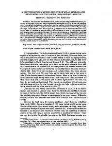
Figure 3: An example for decoding procedure. Table 1: Relevant data.
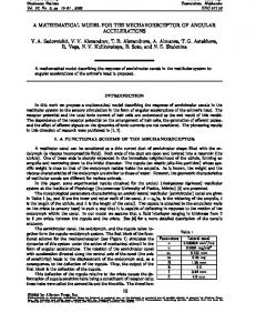
3.2. Solution Representation and Decoding Method. Solution representation involves figuring out a suitable mapping from solutions of problem at hand to individuals in DE population, being the first and foremost issues in using DE for the RMSP problem. Note that DE is initially proposed for continuous optimization problems in which each individual is encoded by float numbers; therefore the priority-based representation is used in this paper in such a way that the feasibility of individuals from parents to offspring can always be ensured. It is worth noting that the priority-based representation resembles the random keys representation that encodes a solution for problem to be optimized with random numbers [30]. Specifically, for priority-based representation, each individual 𝑖 is represented by a list 𝑋𝑖 = {𝑥𝑖1 , 𝑥𝑖2 , . . . , 𝑥𝑖𝑁}, where 𝑖 denotes 𝑖th individual in population, 𝑁 stands for the total number of jobs to be scheduled, and 𝑥𝑖𝑗 (𝑗 = 1, 2, . . . , 𝑁) restricted in [0, 1] is used to indicate the priority of job 𝑗. The larger the value is, the higher priority the job takes. Sort the jobs in a decreasing order of priority; then a complete permutation of all jobs is determined. In order to obtain an intuitive understanding of it, an illustrative instance is shown in Figure 2. The instance comprises 2 reefer mechanics and 6 jobs indexed from 1 to 6, respectively. Job 2 with priority 0.6 is ranked first and thus assigned to be the first element in permutation. By analogy, job 5 is ranked last and is the final
Job ID 𝑟𝑖 𝑝𝑖 𝑑𝑖
1 0 12 19
2 4 10 21
3 8 15 33
4 10 10 28
5 19 12 39
6 20 10 40
job in permutation. In this case, this individual is ultimately interpreted as the job permutation: {2, 1, 4, 3, 6, 5}. Once a permutation is generated, we proceed to decode it into a complete schedule. For this purpose, Algorithm 2 decoding procedure is developed. To explain the decoding method, we also use above instance for illustration. Relevant data is depicted in Tables 1 and 2. In this case, the permutation {2, 1, 4, 3, 5, 6} is decoded into a feasible schedule whose Gantt chart is shown in Figure 3. After decoding, each schedule can be evaluated by a fitness value, inversely proportional to objective value of the schedule. Looking back, we can know that this combination of solution representation and decoding scheme makes DE applicable for the problem under consideration. 3.3. Population Initialization. The quality of initial population is considered to have a great impact on the convergence speed and final solution quality of evolutionary algorithms.
Discrete Dynamics in Nature and Society
5
Step 1: Select the first unscheduled job in the permutation and assign it to the earliest available mechanic, if multiple mechanics are available, then goto Step 2; Step 2: Assign it to the earliest available mechanic with minimum setup time, if multiple mechanics share the minimum setup time, then goto Step 3; Step 3: Assign it to the one with minimum mechanic index; Step 4: Then determine the start time with respect to its release time; Step 5: Repeat Steps 1–4 until all jobs are scheduled. Algorithm 2: Decoding.
Table 2: Setup time. 𝑒𝑖𝑗 1 2 3 4 5 6
1 — 4 5 4 6 4
2 4 — 4 4 4 5
3 5 4 — 6 5 5
4 4 4 6 — 4 4
5 6 4 5 4 — 5
6 4 5 5 4 5 —
Therefore, population initialization is of crucial importance for DE. In the absence of prior knowledge of optimal solutions, we often resort to random initialization which usually results in unsatisfying population. In order to enhance the initial solutions, we make full use of LPT (longest processing time) [31], EDD (Earliest Due Date) [32], and KPM [33] heuristics to generate some high-quality individuals and the remaining is initialized in a random way. Job permutation generated by the adopted heuristics should be encoded into corresponding solution representations. This transition can be realized by the following formula: 𝑋𝐻𝑗 = 1 − (
1 ) (𝑠𝑞𝐻𝑗 − 1) 𝑁
𝑗 = {1, 2, . . . , 𝑁} ,
(11)
where 𝑋𝐻𝑗 , {𝐻 = LPT, EDD, KPM} is the priority of job 𝑗 based on heuristic 𝐻 and 𝑠𝑞𝐻𝑗 is the job index in corresponding permutation. The initial priorities of the remaining individuals are generated within the domain defined by the prescribed interval [0, 1], shown as follows: 𝑋𝑖𝑗 = rand (0, 1) ,
𝑗 = {1, 2, . . . , 𝑁} ,
(12)
where rand(0, 1) is a uniformly distributed random number within the range [0, 1]. 3.4. DE-Based Search. In our algorithm, we implement DE as a main procedure to update the whole population. More specifically, three operators, that is, mutation operator, crossover operator, and selection operator, are executed sequentially to update the population till a preset termination criterion is met. 3.4.1. Mutation Operator. At generation 𝑡, the mutation operator creates a new mutant individual 𝑉𝑖𝑡 with respect to each member 𝑋𝑖𝑡 of the population by a perturbation strategy.
It is widely recognized that the mutation operation plays an important role in determining the performance of DE algorithm. Generally, different mutation strategies are required for different optimization problems depending on the properties of problems. In this regard, we propose an ensemble of mutation strategies for DE algorithm, in which a pool of different mutation strategies coexists throughout the whole search process. Specifically, two distinct mutation operators are employed to construct the strategy pool: (1) Mutation Strategy 1 [23]: “DE/rand/1” 𝑡 𝑡 − 𝑋𝑟3 ), 𝑉𝑖𝑡 = 𝑋𝑟1 + 𝐹 ∗ (𝑋𝑟2
(13)
where 𝑟1 , 𝑟2 , 𝑟3 are mutually exclusive integers randomly selected from [1, 𝑁] and are distinct with 𝑖. 𝐹 is referred to as scaling factor controlling the mutation scale, which is generally distributed in [0, 1]. (2) Mutation Strategy 2: “Gaussian mutation” 𝑉𝑖𝑡 = 𝑁 (𝜇, 𝜎) ,
(14)
where 𝑁(𝜇, 𝜎) is a Gaussian distribution function with mean 𝜇 and standard deviation 𝜎, which are defined by the following formulations: 𝛾1 Best + 𝛾2 𝑋𝑖𝑡 𝛾1 + 𝛾2 𝜎 = 𝜇 − 𝑋𝑖𝑡 , 𝜇=
(15)
where 𝛾1 and 𝛾2 are two random numbers between 0 and 1. Best is the current best individual in population. If the newly generated individual goes beyond bounds [0, 1], we simply reset it within the bounds. The choice between DE/rand/1 and Gaussian mutation is decided by a switch probability and we set it to 0.5 in our algorithm. The reason behind this configuration is that DE/rand/1 has been experimentally proven to possess a strong robustness to different problems. In addition, Gaussian mutation generates new mutant solution based on the current and the best individuals at the present generation. As a result, new mutant individuals will be distributed around the weighted center of 𝑋𝑖𝑡 and Best. At the beginning, the search process emphasizes the global exploration due to the large deviation (initially, 𝑋𝑖𝑡 will be far from Best). As the algorithm proceeds, the deviation becomes smaller, and in this case the search process will focus on local exploitation. Based on the above analysis, this combination is able to
6
Discrete Dynamics in Nature and Society
strike an effective tradeoff between the exploration and exploitation. 3.4.2. Crossover Operator. After mutation, each individual 𝑋𝑖𝑡 along with corresponding mutant individual 𝑉𝑖𝑡 undergoes a crossover operation, through which a new trial individual 𝑈𝑖𝑡 is created. A widely used binomial crossover scheme is defined as follows: 𝑡
{𝑉𝑖𝑗 𝑈𝑖𝑗𝑡 = { 𝑡 𝑋 { 𝑖𝑗
if rand𝑖𝑗 ≤ CR or 𝑗 = 𝑗rand otherwise
(16) 𝑗 = {1, 2, . . . , 𝑁} ,
where rand𝑖𝑗 is a function returning a random number distributed within the range [0, 1]. CR ∈ [0, 1] is named crossover rate which controls how many elements are derived from mutant individual 𝑉𝑖 . 𝑗rand is a random integer chosen from [1, 𝑁] to ensure that the trial individual is distinct with the target individual in at least one element. 3.4.3. Selection Operator. Through mutation and crossover operators, a set of new trial individuals are generated. Subsequently, decoding method is employed to evaluate the fitness values or objective values of all individuals. Finally, a selection operator decides on the survival of trial individual to the next generation, as described by 𝑋𝑖𝑡+1
𝑡 {𝑈𝑖 ={ 𝑋𝑡 { 𝑖
if 𝑓 (𝑈𝑖𝑡 ) ≤ 𝑓 (𝑋𝑖𝑡 ) otherwise.
(17)
{randn (0.75, 0.1) CR𝑖𝑡 = { randn (0.2, 0.1) {
if rand ≤ 0.5 otherwise.
(19)
The meaning of notations in this formula conforms with that of (18). The guideline behind the configuration is that each parameter is sampled from two different normal distributions with the same probability. According to probability theory, distribution with small mean value tends to return a relatively small value which is conductive to intensification, while distribution with large mean value inclines to create a relatively large value which facilitates diversification. In the case, balance between intensification and diversification can be ensured. 3.5. Local Search. When tackling combinatorial optimization problems, incorporating local search into metaheuristic based algorithm with the aim of enhancing exploitation capability is an extremely effective way to strengthen the performance of basic algorithm. In our algorithm, we present two local search strategies. Strategy 1. Three operators, swap, insert, and inverse, are employed in Strategy 1 [34]. Let 𝑋 be the selected individual, and let 𝐴 and 𝐵 be two mutually different positions randomly chosen from [1, 𝑁], respectively; then the steps can be described as follows: (i) Swap (𝑋, 𝐴, 𝐵).
For the problem under consideration, if 𝑈𝑖𝑡 yields a reduction in objective value, then 𝑈𝑖𝑡 replaces 𝑋𝑖𝑡 and survives into the next generation; otherwise 𝑋𝑖,𝑡 is retained. 3.4.4. Parameter Setting. Regarding parameter setting, existing works relevant to DE have demonstrated that its performance is highly sensitive to parameter setting, especially the scaling parameter 𝐹 and the crossover rate CR. And various parameter adaptation strategies have been proposed in previous studies and their effect varies when addressing different issues. We propose a new parameter adapting technique for the purpose of striking a tradeoff between exploration and exploitation. The configuration of 𝐹 is shown by the following equation: {randn (0.4, 0.1) if rand ≤ 0.5 𝐹𝑖𝑡 = { randn (1, 0.1) otherwise, {
Similarly, crossover rate CR is tuned according to another two normal distributions defined as
(18)
where randn represents the normal distribution and the two numbers in bracket indicate mean value and standard deviation, respectively. rand is a random number uniformly distributed within the range [0, 1]. 𝐹𝑖𝑡 will be truncated to [0, 1] if it goes beyond bound constraints.
Swap two elements on positions 𝐴 and 𝐵 in individual 𝑥. (ii) Insert (𝑋, 𝐴, 𝐵). Remove the element on position 𝐴 and then insert it before position 𝐵. (iii) Inverse (𝑋, 𝐴, 𝐵). Inverse the selected subsequence between positions 𝐴 and 𝐵. Step 1. Select the best individual. Step 2. Sequentially perform swap, insert, and inverse operator on it, 𝑗. Step 3. Return a new individual. After these operations are sequentially executed, a new individual is generated and competes with 𝑋 to survive. It is worth mentioning that we implement local search directly on the encoding individual rather than its corresponding permutation, to avoid wasteful duplication of conversion between permutation and individual. In addition, we only perform local search on the best individual to save computational resource.
Discrete Dynamics in Nature and Society
7
1
2
3
4
5
6
0.50
0.60
0.30
0.40
0.10
0.20
1
M2
4
6
Swap (X, 5, 6) 1
2
3
4
5
6
0.50
0.60
0.40
0.30
0.20
0.10
2
M1
Insert (X, 4, 1)
0
1
2
3
4
5
6
0.30
0.50
0.60
0.40
0.20
0.10
1
2
3
4
5
6
0.60
0.50
0.30
0.40
0.20
0.10
M1
3
4
5
6
15
20
5
25
5
30
35
40
3
1
0 2
10
2
M2
Inverse (X, 1, 3)
1
5
3
15
20
50
45
50
6
4
10
45
5
25
30
35
40
Permutation
Figure 4: An illustrative example for local search Strategy 1.
An example is illustrated for the operators in Figure 4. Suppose that we aim at improving the individual {0.50, 0.60, 0.30, 0.40, 0.10, 0.20} whose objective is 21.5 and the corresponding Gantt chart is shown in the top right of Figure 4. By performing the proposed local search Strategy 1, a new individual {0.60, 0.50, 0.30, 0.40, 0.20, 0.10} is generated with objective being 20 and the corresponding Gantt chart is depicted in the bottom right of Figure 4. Noticeably, the new individual survives into the next generation. In this regard, the proposed local search strategy has the potential to improve the quality of incumbent solutions.
Strategy 2. In view of the superiority of NEH heuristic for the PFSP [35], we extend it and propose another insert-based local search strategy. Similarly, we perform it only on the best individual; the main procedures are listed as follows: Step 1. Decode the best individual into job permutation. Step 2. Find out the first available mechanic 𝑗. Insert 𝑖th job 𝑖 = 1, 2, . . . , 𝑛 in every position before and after any previously. Step 3. Schedule job on the selected mechanic 𝑗 and schedule the job in the position with lowest resulting objective function value. Step 4. Repeat Steps 2 and 3 until all jobs are scheduled.
If the new schedule is superior to the predetermined one, we will accept it as the new best schedule. Afterwards, we should convert the new best schedule into an individual, which is a reverse process of decoding. The conversion has two phases: (1) transform the schedule into job permutation (see Algorithm 3); (2) then transform corresponding permutation into individual according to (11). 3.6. Procedure of the Proposed Algorithm. In this paper, we encode a solution with priority and develop a new parameter setting strategy to balance exploration and exploitation abilities of DE. Additionally, two local search strategies along with a new Gaussian mutation are integrated into DE for performance improvement. The steps of the resulting algorithm are shown in Algorithm 4.
4. Computational Experiments In order to validate the performance of the proposed DE algorithm, we have conducted comprehensive experiments on a suite of randomly generated instances. The MIP formulation is solved by the CPLEX 12.5 solver implemented in MATLAB R2014a. The proposed algorithm is also coded in MATLAB and run on a Core i3 computer (2.3 GHz) with 4 GB of memory. To test the effectiveness of local search strategies, we compare it with other algorithmic techniques reported in literature, that is, GA, genetic algorithm [21], and IH, insert-based heuristic [22].
8
Discrete Dynamics in Nature and Society
Step 1: Step 2:
Step 3: Step 4:
Let 𝐴 𝑖 , {𝑖 = 1, 2, . . . , 𝑀} be the set of scheduled jobs on mechanic 𝑖, initialize corresponding earliest available time 𝐹𝑖 to 0, calculate minimum earliest available time 𝐹 and set initial permutation 𝑃 = 0; Identify the mechanic 𝑘, 𝑘 ∈ {1, 2, . . . , 𝑀} Step 2.1 Select mechanic 𝑘 such that 𝐹𝑘 = 𝐹, if multiple mechanics satisfy this, then goto Step 2.2; Step 2.2 For each mechanic 𝑘, compute 𝐹𝑘 = 𝐹𝑘 + the setup time for first job in 𝐴 𝑘 , then select mechanic 𝑘 with minimum 𝐹𝑘 , if multiple mechanics satisfy this, then goto Step 2.3 Step 2.3 Select the mechanic with minimum mechanic index. Delete the first job in 𝐴 𝑘 and append it to P, update 𝐴 𝑘 , 𝐹𝑖 and 𝐹. If 𝐴 𝑖 = 0, then mechanic 𝑖 is not in consideration in further iterations; Repeat Steps 2 and 3, until a complete permutation is derived. Algorithm 3: Transform schedule into job permutation.
Step 1: Initialize: Step 1.1 Initialize three individuals by LPT, EDD and KPM heuristics; Step 1.2 Generate the rest in a random way; Step 2: Evaluate each solution and record the best one; While Stop condition is met, output the best result, otherwise Do Step 3: Perform DE-based search: Step 3.1: Mutation Create a mutant population 𝑉; Step 3.2: Crossover Recombine mutant population 𝑉 and target population 𝑋 to produce a new trial population 𝑈; Step 3.3: Selection Update population by one-to-one greedy selection; Step 4: Perform local search on the current best: Step 4.1: Execute Strategy 1; Step 4.2: Update the best individual; Step 4.3: Execute Strategy 2; Step 4.4: Update the best individual; End Algorithm 4: Proposed DE.
4.1. Instance Generation. Since there is no benchmark available for the RMSP problem, instances are randomly created for different numbers of jobs and mechanics, represented by 𝑛/𝑚. The related data are generated in the following ways: (i) 𝑁 ∈ {8, 20, 30, 40, 50, 60}, 𝑀 ∈ {2, 4, 6, 8, 10}. (ii) The release times are random integers in the range [0, 20]. (iii) The processing times take values from the uniform distribution over [10, 30]. (iv) The setup times are also integers uniformly sampled from 4 to 6 which are 10∼30% of the mean value of the processing time. (v) The due dates are computed by 𝑑𝑖 = 𝑟𝑖 + 𝑝𝑖 + RD ∼ [6, 10], where RD ∼ [6, 10] means that a random integer is generated in the interval [6, 10] with equal probability. (vi) The weight of the total walking distance in the objective function is assumed to be 0.5.
Five instances are generated for each combination (𝑛, 𝑚), yielding 150 instances in total. The raw data are available by request to the corresponding author through e-mail. 4.2. Lower Bound. Heuristic algorithms report solutions whose optimality could not always be confirmed. In view of this, we decide to evaluate the quality of solutions via comparing them with lower bound LB. To derive the lower bound, we relax the instance under examination by reassociating the minimum value of setup times among jobs with each job. In this case, the setup time can be viewed as a given increment in processing time for convenience. Moreover, the second term in objective function indicating the total walking distance of all mechanics becomes a constant. Therefore, the relaxed problem can be remodeled by a time indexed formulation. It is worth noting that it is technically difficult to formulate original RMSP by a time indexed formulation due to the presence of different setup times. 𝑇 denotes the upper bound of the makespan of each instance. Variable 𝑥𝑖𝑡 is equal to 1 if job 𝑖 starts at time 𝑡, 0 otherwise. Assume that 𝑠 is the
Discrete Dynamics in Nature and Society
9
minimum of setup times and 𝑚 ≤ 𝑛; then the formulation is shown as follows: min 𝑍LB = ∑ ∑ 𝑥𝑖𝑡 max (0, 𝑡 + 𝑝𝑖 − 𝑑𝑖 ) 𝑖∈𝑁 𝑡∈[0,𝑇]
(20)
+ 𝛼 (𝑛 − 𝑚) 𝑠 s.t.
𝑥𝑖𝑡 = 0, ∑
𝑖 ∈ 𝑁, 𝑡 ≤ 𝑟𝑖 ∑
𝑖∈𝑁 𝑡∈[𝑡−𝑝𝑖 −𝑠+1,𝑡]
𝑥𝑖𝑡 ≤ 𝑚,
∑ 𝑥𝑖𝑡 = 1, 𝑖 ∈ 𝑁
𝑡∈[0,𝑇]
(21) 𝑡 ∈ [0, 𝑇]
(22)
𝑛/𝑚 8/2 8/4 8/6 8/8 8/10 Average
DE 0 0 0 0 0 0
(23)
𝑥𝑖𝑡 ∈ {0, 1} , where constraints (21) restrict that each job cannot be processed before its release time. Constraints (22), referred to as resource constraints, state that at most 𝑚 jobs can be executed simultaneously. Constraints (23) ensure that each job should begin once and only once. Constraints (24) clarify the domains of variables. The lower bound for original problem is obtained by solving above formulation using CPLEX solver. It is worth mentioning that a fair comparison among the three heuristic algorithms is assured through executing all algorithms for the same number of objective function evaluations: 400 × 𝑛 (for small size problems) and 2000 × 𝑛 (for large size problems) in a run, where 𝑛 is the number of jobs. That is to say, when the maximum of fitness function evaluations is reached, the execution of a particular algorithm is stopped. The parameter 𝑝𝑜𝑝𝑠𝑖𝑧𝑒 is set to 40 in a 𝐹𝑜𝑟 𝐿𝑜𝑜𝑝 of DE algorithm. Other two algorithms follow the setting described in their respective literature. Five independent runs are carried out for each algorithm in each problem instance and the best result from the five repeated runs is accepted as the final solution to the problem instance. 4.3. Computational Results and Analysis 4.3.1. Results for Small Size Problems. Since the time and space complexities of exact solution methods exponentially grow with the increase in problem size, the CPLEX solver can only solve the MIP formulation containing 8 jobs to optimality on a computer introduced above in our experiments. The solver runs out of memory when we proceed to larger size problems. Therefore, we use the 8-job problem instances, named small size problems, to demonstrate the performance of proposed DE algorithm and its competitiveness to other heuristics. The metric for evaluating the performance is to
IH 5.21 15.87 66.25 0 0 29.11
∑5𝑖=1 PD (𝑖) , 5
(25)
where PD = 100 (
(24)
GA 0 0 0 0 0 0
compute a mean percentage deviation of the solution from optimal solution by the following formula: MPD =
𝑡 ∈ [0, 𝑇] , 𝑖 ∈ 𝑁,
Table 3: Mean percent deviation for small size problems.
𝑂𝐴 (𝑖) − 𝑂𝑜 (𝑖) ), 𝑂𝑜 (𝑖)
𝑖 = 1, 2, . . . , 5,
(26)
where 𝑂𝐴 (𝑖) is the final solution obtained from a given algorithm 𝐴 and 𝑂𝑜 (𝑖) is the optimal solution reported by CPLEX solver for 𝑖th problem instance of a specific combination (𝑛, 𝑚). PD(𝑖) is the corresponding percentage deviation. Obviously, lower value of MPD is preferred. The computational results for small size problems are summarized in Table 3. Lowest MPD value is identified with boldface for each combination. According to the results shown in Table 3, the proposed DE algorithm and GA are the best-performing algorithms among the three heuristics in terms of MPD values. MPD of 0% suggests that both DE and GA can solve all the small size problem instances to optimality. We can observe that insert-based heuristic produces the worst MPD compared to its counterparts, which verifies that rule-base heuristic often yields less satisfactory results. Therefore, it can be concluded that the overall ranking of three heuristic algorithms from best to worst is as follows: DE, GA, and IH. To demonstrate the efficiency of the proposed DE algorithm, we trace the track of the best objective values found by DE and GA with respect to function evaluation over an instance of combination (8, 4), as shown in Figure 5. It is obvious that DE is the best one in terms of convergence speed, concluding that DE is computationally efficient in solving small size problems to optimality. 4.3.2. Results for Large Size Problems. Since there do not exist exact algorithms capable of finding optimal solutions within a reasonable amount of time, we now assess the performance of aforementioned approaches for large size problems by computing a relative mean percentage deviation of best solutions from lower bound LB as follows: MPD =
∑5𝑖=1 PD (𝑖) , 5
(27)
where PD = 100 (
𝑂𝐴 (𝑖) − LB (𝑖) ), LB (𝑖)
𝑖 = 1, 2, . . . , 5,
(28)
10
Discrete Dynamics in Nature and Society 62
Table 4: Mean percent deviation for large size problems.
Objective value
60 58 56 54 52 50 48
×40
0
10
20
30 40 50 Function evaluations
60
70
80
GA DE
Figure 5: Track of the best solutions.
where 𝑂𝐴 (𝑖) represents the best result from five replications for a specific algorithm 𝐴 and LB(𝑖) is the lower bound of instance 𝑖. PD(𝑖) is the corresponding percentage deviation. Similarly, for a given algorithm, the lower its MPD, the better its capability. All the computational results are listed in Table 4. As we can see from Table 4, the three heuristics show a distinct difference in finding optimal or approximate optimal solutions. The proposed DE algorithm obtains the lowest MPDs and thus is superior to other algorithms in terms of solution quality. Obviously, DE algorithm yields best results with average MPDs being less than 2.00% for all combinations. The performance of GA is relatively satisfactory with average MPDs being less than 5.50% for all combinations. However, IH is noticeably inferior to DE and GA in solution quality. Moreover, the results take lower bound as benchmark; hence the best solutions found by DE can be even closer to optimal ones by large probability. From a practical point of view, the results obtained by DE are very encouraging and indicate that DE algorithm is viable for large size problems. Interestingly, we can notice that there is a tendency that for a given number of jobs the MPD slightly increases as the number of mechanics increases with only a few exceptions. A possible reason for this expected phenomenon might be that the search space (solution space) enlarges gradually as the number of mechanics grows. So, we can infer that the number of mechanics is probably the determinant of hardness of problems under consideration. Due to the limitation of space, herein, we only illustrate the convergence speed of DE over one instance of combination (30, 4). Figure 6 plots the best solution found during entire iterative process. For comparison, we also record the convergence process of GA. Clearly, the convergence of DE is very satisfactory because it consumes about 1 × 10⁴ function evaluations to converge to an approximate solution. Moreover, the difference of deviation between 1 × 10⁴ function evaluations and 1.5 × 10⁴ function evaluations is very marginal. GA is also excellent in efficiency but encounters a dilemma in achieving a good solution. In summary, this graph confirms that DE algorithm is effective and efficient in dealing with RMSP problems.
𝑛/𝑚 20/2 20/4 20/6 20/8 20/10 Average 30/2 30/4 30/6 30/8 30/10 Average 40/2 40/4 40/6 40/8 40/10 Average 50/2 50/4 50/6 50/8 50/10 Average 60/2 60/4 60/6 60/8 60/10 Average
DE 1.59 2.00 0.91 3.97 8.35 3.36 1.44 1.47 1.66 2.36 1.83 1.75 1.12 1.68 1.89 1.89 2.40 1.79 1.05 1.59 2.19 2.30 2.14 1.85 0.86 1.41 1.93 2.15 2.86 1.84
GA 2.71 4.81 2.65 5.71 9.48 5.14 2.67 4.00 5.05 5.08 4.29 4.22 2.07 4.13 3.71 4.66 5.95 4.10 2.39 2.64 3.79 5.22 5.33 3.87 2.19 3.09 4.29 5.15 5.57 4.05
IH 4.38 8.62 10.75 29.94 32.06 11.16 3.14 4.95 7.14 13.20 12.14 8.11 2.10 4.50 5.48 6.52 8.58 5.40 1.91 2.69 4.28 5.92 6.13 4.19 1.25 2.51 4.30 5.42 6.97 4.09
4.3.3. A Summary of Experimental Results. In this section, we present an overall analysis of the proposed algorithm and the existing algorithms in literature. The experimental results on different sized problems in the previous section demonstrate that the proposed DE algorithm is advantageous over IH and GA in terms of solution quality. Moreover, the proposed algorithm converges faster than GA. Specifically, for smallscale instances, the proposed algorithm and GA dominate IH when solution quality (MPD) is considered. Both of them can produce optimal solutions with 0 MPDs while the average MPD obtained by IH is 29.11%. As for large size problems, the proposed algorithm is superior to GA and IH. The proposed algorithm reports solutions without optimality guarantee but still produces the comparatively best-quality with the worst MPD less than 8.35%. On average, the MPD is reduced by 2.2% and 4.5% as compared with those obtained from GA and IH, respectively. Furthermore, the convergence curves indicate that the proposed algorithm converges to a better solution in much less function evaluations. The superior performance of the proposed DE algorithm may stem from two aspects: (1) LPT, EDD, and KPM heuristics
Discrete Dynamics in Nature and Society
11
Table 5: Mean percent deviation for DE and its variants. 𝑛/𝑚 8/2 8/4 8/6 8/8 8/10 Average 20/2 20/4 20/6 20/8 20/10 Average 30/2 30/4 30/6 30/8 30/10 Average 40/2 40/4 40/6 40/8 40/10 Average 50/2 50/4 50/6 50/8 50/10 Average 60/2 60/4 60/6 60/8 60/10 Average
DE 0 0 0 0 0 0 1.59 2.00 0.91 3.97 8.35 3.36 1.44 1.47 1.66 2.36 1.83 1.75 1.12 1.68 1.89 1.89 2.21 1.758 1.05 1.59 2.19 2.30 2.14 1.85 0.86 1.41 1.93 2.15 2.86 1.84
DE-M 0 0 0 0 0 0 1.63 2.00 0.94 3.97 8.35 3.37 1.78 2.32 2.17 3.06 2.17 2.30 1.43 2.35 2.45 2.81 3.15 2.43 1.19 2.11 2.61 3.02 3.48 2.48 1.08 1.68 2.78 2.95 3.59 2.42
provide DE algorithm with a good initial population; (2) the configuration of parameter and mutation operator and local search strategies can establish a good balance between two forces: intensification and diversification. However, GA tends to suffer from stagnation of the search process due to the diversity loss, which explains why it yields less competitive solutions than the proposed algorithm. Based on the comparisons, we can conclude that the proposed DE algorithm is more effective than existing approaches in solving the RMSP. 4.3.4. Effectiveness of the Improvement Strategies. The primary improvement strategies presented in Section 3 include the new mutation mechanism, the two local search strategies, and the new parameter setting method. The purpose of this
DE-LS1 0 0 0 0 0 0 1.59 2.50 1.15 4.18 8.35 3.55 1.76 1.94 1.88 2.75 3.82 2.43 1.27 1.96 1.86 2.79 3.06 2.18 1.26 2.63 2.97 3.37 3.31 2.70 1.13 1.94 2.95 3.17 3.56 2.55
DE-LS2 0 0 0 0 0 0 1.84 2.24 1.27 3.97 8.35 3.53 1.53 1.80 1.66 2.57 2.41 1.99 1.37 1.76 2.19 2.34 3.15 2.16 1.26 1.83 2.26 2.88 2.95 2.23 1.04 1.85 2.99 2.53 3.41 2.364
DE-P 0 0 0 0 0 0 1.84 2.46 1.41 5.32 9.15 4.03 1.62 2.13 2.75 3.73 2.23 2.49 1.28 2.18 2.04 2.29 2.34 2.03 1.17 1.60 2.25 2.60 2.57 2.03 0.81 1.50 1.94 2.90 2.92 2.014
subsection is to verify the effectiveness of the above components. To this end, additional comparative experiments were executed for different variants of the proposed DE. They are enumerated as follows: (1) DE without new mutation mechanism and with only DE/rand/1, denoted as DE-M; (2) DE without local search Strategy 1, denoted as DE-LS1; (3) DE without local search Strategy 2, denoted as DE-LS2; and (4) DE without new parameter setting method, denoted as DE-P. For DE-P, 𝐹 is set to 0.4 and CR to 0.7 after extensive computational experiments. We follow a similar computational procedure to that explained before. The experimental results of DE, DE-M, DE-LS1, DE-LS2, and DE-P are reported in Table 5, where the best results for each combination are highlighted in boldface.
12
Discrete Dynamics in Nature and Society generate 𝑂(𝑛𝑇) 0-1 variables. Note that an optimal solution has only 𝑛 variables set to 1 and remaining to 0. Therefore, it is worthwhile to use column generation to solve the time indexed formulation more efficiently. Moreover, another desired extension of the current work is to take into consideration the uncertainty in release times, conforming to more practical scenarios.
2100
Objective values
2050 2000 1950 1900 1850
Competing Interests
1800 1750
×40
0
500 1000 Function evaluations
1500
GA DE
Figure 6: Track of the best solutions.
We can observe in Table 5 that there is no distinct difference in performance for these algorithms with regard to small size problems. Nevertheless, when it comes to large size ones, the difference becomes obvious. The proposed DE obtains the best overall results, in comparison with all other algorithms. Removal of any one of these components will generally trigger a significant degeneration in performance. We attribute this phenomenon to the fact that all these improvement strategies are vital for a better balance between the exploration and exploitation during the evolution. Therefore, we can conclude that the above components can collaboratively enhance the performance of basic DE algorithm.
5. Conclusion In this work, we consider the problem of scheduling reefer mechanics to minimize the sum of the total tardiness of all reefers and the total walking distance of all mechanics and we formulate it as mixed integer programming. Considering the NP-hardness of the problem, we propose a DE algorithm to solve it. First, to make DE suitable for the problem, priority-based representation is used. Second, LPT, EDD, and KPM heuristics are used in combination with random initialization to alleviate the search randomness at the beginning and get a high-quality initial population. Third, balance between diversification and intensification is ensured by welldesigned crossover operator, parameter setting, and local search scheme. Then, the resulting algorithm is compared against other two constructive heuristics and thoroughly tested on small size and large size problems, respectively. The results suggest that the proposed algorithm outperforms the existing IH and GA algorithms and it is effective and efficient in finding optimal or approximate optimal solutions for the RMSP. In future work, on one hand, the time indexed formulation for calculating lower bound suffers from a low efficiency for large sized problems when solved by CPLEX solver, resulting from extremely large amount of efforts to
The authors declare that there is no conflict of interests regarding the publication of this paper.
Acknowledgments This work was supported by the National Natural Science Foundation of China (Grant nos. 71271138, 71101106, and 71428002).
References [1] D.-H. Lee, H. Q. Wang, and L. Miao, “Quay crane scheduling with non-interference constraints in port container terminals,” Transportation Research Part E: Logistics and Transportation Review, vol. 44, no. 1, pp. 124–135, 2008. [2] M. Liu, F. Chu, Z. Zhang, and C. B. Chu, “A polynomialtime heuristic for the quay crane double-cycling problem with internal-reshuffling operations,” Transportation Research Part E: Logistics and Transportation Review, vol. 81, pp. 52–74, 2015. [3] C.-Y. Lee, M. Liu, and C. Chu, “Optimal algorithm for the general Quay crane double-cycling problem,” Transportation Science, vol. 49, no. 4, pp. 957–967, 2015. [4] K. H. Kim, “An optimal routing algorithm for a transfer crane in port container terminals,” Transportation Science, vol. 33, no. 1, pp. 17–33, 1999. [5] I. Vacca, M. Salani, and M. Bierlaire, “An exact algorithm for the integrated planning of berth allocation and quay crane assignment,” Transportation Science, vol. 47, no. 2, pp. 148–161, 2013. [6] A. Imai, K. Sasaki, E. Nishimura, and S. Papadimitriou, “Multiobjective simultaneous stowage and load planning for a container ship with container rehandle in yard stacks,” European Journal of Operational Research, vol. 171, no. 2, pp. 373–389, 2006. [7] I. F. A. Vis and H. J. Carlo, “Sequencing two cooperating automated stacking cranes in a container terminal,” Transportation Science, vol. 44, no. 2, pp. 169–182, 2010. [8] A. Lim and Z. Xu, “A critical-shaking neighborhood search for the yard allocation problem,” European Journal of Operational Research, vol. 174, no. 2, pp. 1247–1259, 2006. [9] R. Stahlbock and S. Voß, “Operations research at container terminals: a literature update,” OR Spectrum, vol. 30, no. 1, pp. 1–52, 2008. [10] C. Bierwirth and F. Meisel, “A survey of berth allocation and quay crane scheduling problems in container terminals,” European Journal of Operational Research, vol. 202, no. 3, pp. 615–627, 2010. [11] H. J. Carlo, I. F. A. Vis, and K. J. Roodbergen, “Seaside operations in container terminals: literature overview, trends, and
Discrete Dynamics in Nature and Society
[12]
[13]
[14]
[15]
[16]
[17]
[18]
[19]
[20]
[21]
[22]
[23]
[24]
[25]
[26]
research directions,” Flexible Services and Manufacturing Journal, vol. 27, no. 2-3, pp. 224–262, 2015. M. Liu, Y. Xu, C. Chu, and F. Zheng, “Online scheduling to minimize modified total tardiness with an availability constraint,” Theoretical Computer Science, vol. 410, no. 47-49, pp. 5039–5046, 2009. C. Chu, “A branch-and-bound algorithm to minimize total tardiness with different release dates,” Naval Research Logistics (NRL), vol. 39, no. 2, pp. 265–283, 1992. F. Yalaoui and C. Chu, “Parallel machine scheduling to minimize total tardiness,” International Journal of Production Economics, vol. 76, no. 3, pp. 265–279, 2002. I. Kacem, N. Souayah, and M. Haouari, “Branch-and-bound algorithm for total weighted tardiness minimization on parallel machines under release dates assumptions,” RAIRO Operations Research, vol. 46, no. 2, pp. 125–147, 2012. J. M. J. Schutten and R. A. M. Leussink, “Parallel machine scheduling with release dates, due dates and family setup times,” International Journal of Production Economics, vol. 46-47, pp. 119–125, 1996. Z.-L. Chen and C.-Y. Lee, “Parallel machine scheduling with a common due window,” European Journal of Operational Research, vol. 136, no. 3, pp. 512–527, 2002. T.-C. Chiang, H.-C. Cheng, and L.-C. Fu, “A memetic algorithm for minimizing total weighted tardiness on parallel batch machines with incompatible job families and dynamic job arrival,” Computers and Operations Research, vol. 37, no. 12, pp. 2257–2269, 2010. S. A. Torabi, N. Sahebjamnia, S. A. Mansouri, and M. A. Bajestani, “A particle swarm optimization for a fuzzy multiobjective unrelated parallel machines scheduling problem,” Applied Soft Computing Journal, vol. 13, no. 12, pp. 4750–4762, 2013. J. Lamothe, F. Marmier, M. Dupuy, P. Gaborit, and L. Dupont, “Scheduling rules to minimize total tardiness in a parallel machine problem with setup and calendar constraints,” Computers & Operations Research, vol. 39, no. 6, pp. 1236–1244, 2012. S. Hartmann, “A general framework for scheduling equipment and manpower at container terminals,” in Container Terminals and Automated Transport Systems, pp. 207–230, Springer, Berlin, Germany, 2005. S. Hartmann, “Scheduling reefer mechanics at container terminals,” Transportation Research Part E: Logistics and Transportation Review, vol. 51, no. 1, pp. 17–27, 2013. R. Storn and K. Price, “Differential evolution—a simple and efficient heuristic for global optimization over continuous spaces,” Journal of Global Optimization, vol. 11, no. 4, pp. 341– 359, 1997. A. Ponsich and C. A. C. Coello, “A hybrid differential evolution—Tabu Search algorithm for the solution of job-shop scheduling problems,” Applied Soft Computing Journal, vol. 13, no. 1, pp. 462–474, 2013. D. Chen, E. Cao, and W. Lai, “A differential evolution algorithm for pickups and deliveries problem with fuzzy time windows,” Journal of Intelligent & Fuzzy Systems, vol. 30, no. 1, pp. 267–277, 2016. L. Wang, Y. Zeng, and T. Chen, “Back propagation neural network with adaptive differential evolution algorithm for time series forecasting,” Expert Systems with Applications, vol. 42, no. 2, pp. 855–863, 2015.
13 [27] P. Yan, G. Wang, A. Che, and Y. Li, “Hybrid discrete differential evolution algorithm for biobjective cyclic hoist scheduling with reentrance,” Computers and Operations Research, vol. 76, pp. 155–166, 2016. [28] W. S. Sakr, R. A. EL-Sehiemy, and A. M. Azmy, “Adaptive differential evolution algorithm for efficient reactive power management,” Applied Soft Computing, vol. 53, pp. 336–351, 2017. [29] S. Zhou, M. Liu, H. Chen, and X. Li, “An effective discrete differential evolution algorithm for scheduling uniform parallel batch processing machines with non-identical capacities and arbitrary job sizes,” International Journal of Production Economics, vol. 179, pp. 1–11, 2016. [30] E. Koyuncu and R. Erol, “PSO based approach for scheduling NPD projects including overlapping process,” Computers and Industrial Engineering, vol. 85, pp. 316–327, 2015. [31] J. Adams, E. Balas, and D. Zawack, “The shifting bottleneck procedure for job shop scheduling,” Management Science, vol. 34, no. 3, pp. 391–401, 1988. [32] L. J. Wilkerson and J. D. Irwin, “An improved method for scheduling independent tasks,” A I I E Transactions, vol. 3, no. 3, pp. 239–245, 1971. [33] C. Koulamas, “Decomposition and hybrid simulated annealing heuristics for the parallel-machine total tardiness problem,” Naval Research Logistics, vol. 44, no. 1, pp. 109–125, 1997. [34] B. Liu, L. Wang, and Y.-H. Jin, “An effective PSO-based memetic algorithm for flow shop scheduling,” IEEE Transactions on Systems, Man, and Cybernetics, Part B: Cybernetics, vol. 37, no. 1, pp. 18–27, 2007. [35] M. Nawaz, E. E. Enscore Jr., and I. Ham, “A heuristic algorithm for the m-machine, n-job flow-shop sequencing problem,” Omega, vol. 11, no. 1, pp. 91–95, 1983.
Advances in
Operations Research Hindawi Publishing Corporation http://www.hindawi.com
Volume 2014
Advances in
Decision Sciences Hindawi Publishing Corporation http://www.hindawi.com
Volume 2014
Journal of
Applied Mathematics
Algebra
Hindawi Publishing Corporation http://www.hindawi.com
Hindawi Publishing Corporation http://www.hindawi.com
Volume 2014
Journal of
Probability and Statistics Volume 2014
The Scientific World Journal Hindawi Publishing Corporation http://www.hindawi.com
Hindawi Publishing Corporation http://www.hindawi.com
Volume 2014
International Journal of
Differential Equations Hindawi Publishing Corporation http://www.hindawi.com
Volume 2014
Volume 2014
Submit your manuscripts at https://www.hindawi.com International Journal of
Advances in
Combinatorics Hindawi Publishing Corporation http://www.hindawi.com
Mathematical Physics Hindawi Publishing Corporation http://www.hindawi.com
Volume 2014
Journal of
Complex Analysis Hindawi Publishing Corporation http://www.hindawi.com
Volume 2014
International Journal of Mathematics and Mathematical Sciences
Mathematical Problems in Engineering
Journal of
Mathematics Hindawi Publishing Corporation http://www.hindawi.com
Volume 2014
Hindawi Publishing Corporation http://www.hindawi.com
Volume 2014
Volume 2014
Hindawi Publishing Corporation http://www.hindawi.com
Volume 2014
Discrete Mathematics
Journal of
Volume 2014
Hindawi Publishing Corporation http://www.hindawi.com
Discrete Dynamics in Nature and Society
Journal of
Function Spaces Hindawi Publishing Corporation http://www.hindawi.com
Abstract and Applied Analysis
Volume 2014
Hindawi Publishing Corporation http://www.hindawi.com
Volume 2014
Hindawi Publishing Corporation http://www.hindawi.com
Volume 2014
International Journal of
Journal of
Stochastic Analysis
Optimization
Hindawi Publishing Corporation http://www.hindawi.com
Hindawi Publishing Corporation http://www.hindawi.com
Volume 2014
Volume 2014