Proceedings of the World Congress on Engineering 2013 Vol I, WCE 2013, July 3 - 5, 2013, London, U.K.
Mathematical Modeling and Algorithms to Simulate The Economy's Behavior Sameh Abdelwahab Eisa, Belal Mostafa Amin Abstract—in this paper we are proposing continuous mathematical modeling for describing the economic behavior and the relations between its components, as a system of PDEs. We deduced two algorithmic procedures, which allow us to forecast and simulate the economic behavior as a whole (GDP) and the impacts of each component on the other components. We have shown results, which support our hypotheses. We introduced flow-charts for the algorithms and complete results as a simulation to clarify our progress. Through these algorithms we will be able to simulate the economy for any country or economic entity and allow the simulators to consider changes, and then they can notice the future results according to these changes. We have assumed a model for "The Unemployment" and how it changes according to the changes in the economic components. Index Terms—Forecasting economy behavior, Mathematical modeling, economic modeling, Unemployment model, Algorithm, GDP, Investment, Consumption, Governmental Expenditure, Exports, Imports, Economic components, Economic modeling, Mathematical modeling for economy, Partial Differential Equation, Differential Equations, Difference Equations, Economy simulation, Simulation.
for specific economic component and its effects on the other components, As well as, we will introduce algorithmic procedure to execute these purposes, and we will clarify to the scientific community, the ability of analyzing the relation between something like "The Unemployment" and the economic components. II. IDEA OF THE MODEL We will propose mathematical model that depends on some logical assumptions, in order to deduce algorithmic procedures, which allow us to simulate the economic behavior and enable us to establish methods for forecasting the changes in the economy's components. During the research, we are using data of United States as a material for our experiments and simulations; we have cited the sources of the data in the references.
A. Basic assumptions 1-
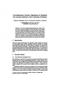
GDP of a country can be expressed in terms of many components, which are well known for economists. As a result, GDP's components can be represented in a tree form like figure (1).
I. INTRODUCTION THE economic problems and their impacts on man's life occupy wide area on scientists minds, because after all, the people are facing the impacts of these problems daily. Therefore, these dilemmas are driving the scientists from all specialties to contribute as they could to find solutions. The mathematicians and the engineers are not far from theses attempts, because there is substantial necessity for describing the economy and the relations between its components logically and mathematically. We thought that deducing differential/difference equation to describe the relation between the economic components for any country or economic entity will be the start. We have searched carefully to see if there are some attempts in this path, to be aware of them. We have cited number of published works in the last decade, which were digging on this subject. For examples, Tomáš Škovránek, Igor Podlubny, Ivo Petráš in [8] tried to made modeling in state space using fractional calculus approach, Christian Schumacher, Jörg Breitung in [3] were using quarters and years data in order to forecast Germany's GDP using their model, like them, the authors in [7] who tried to forecast Latin Americas GDPs, We carefully looked on the models' ideas which are proposed through [6], [2] and [9] to be aware of their ideas and to be sure about our originality. We also have cited some online links for statistics data, which essentially helped us through our research. We are proposing a logical model, which depends on known mathematical identities and some hypotheses to study the changes Sameh Abdelwahab Eisa, known as SAN Eisa, is an applied mathematician and researcher, master student with several publications, from Egypt,
[email protected] Belal Mostafa Amin, is a student in communication and computer department in the faculty of engineering, interested in research in applied mathematics, from Egypt.
[email protected]
ISBN: 978-988-19251-0-7 ISSN: 2078-0958 (Print); ISSN: 2078-0966 (Online)
Figure.1 Tree of GDP and its components
2-
Each component in this tree will be considered as a function of the other components. We are building this assumption on the principle, that all the economic components are connected with the man, so any change in any component by/for the man, will affect each of the other components individually and GDP generally. For example, if we consider the first line in the tree, (1) Then,
(2)
3-
and the same for every considered row in the tree. Each country or economic entity has its own economic environment, so we will deduce the functions in (2) by fitting the provided data (years or quarters) to find suitable functions for each specific environment. We will perform the known methods of regression and interpolation "Least square methods" by applying polynomial, exponential, power and linear models. Its highly expected that, relations between two variables in a country can be different from the relations between in other country, because of the character of each economy.
WCE 2013
Proceedings of the World Congress on Engineering 2013 Vol I, WCE 2013, July 3 - 5, 2013, London, U.K. 4-
It's hard to make the fitting between a component and all the others in multidimensional variables, so we will deduce the fittings between every two components separately, to determine specified relation, for example, then To deduce we will deduce fitting between determine the derivative.
B. Fundamental relations and derivations By considering a general row from the GDP's tree (their summation must equal ). (3) Where is representing specific component in chosen row in the tree presented in figure (1). Then, (4) According to assumption 2 and (2), we can deduce the below equations by using the chain rule. (5) Where is the number of components in specific row. We can construct equations for every using the same concepts.
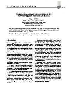
Figure.3 GDP of US from 1948-2011 by exponential fitting
We will replace each of the time derivatives for each component and for in the right hand side of (5) & (6) by known functions. These functions results from the differentiation of the interpolated function, which deduced from the fitting with time. Consequently, we will assume the below (8)
(6) These modifications will generate system of PDEs which describe the relations between the components depending on the hypothesis in (2). We can apply the finite difference technique on the other terms in the right hand side of (5) & (6) then,
Then we can collect equations from (5) and (6). According to a lot of experiments, the fitting of and the components versus time brings high efficient results and high values of (coefficient of determination), (7)
The fitting of the power model
Fitting value of the poly 2nd degree
Linear Regression Fitting values
Exponential Fitting Value
Component Name
Considering 5 quarters
Where is the theoretical y-value corresponding to (calculated through the model) and is the mean value of all experimental yvalues and is the number of years or quarters in which the data represented. some of the results are shown in table(1), figures (2),(3).
GDP 0.8572 0.8570 0.8599 0.8237 C 0.9886 0.9886 0.9886 0.9505 I 0.8924 0.8961 0.9189 0.8802 G 0.9922 0.9909 0.9944 0.9273 X 0.8592 0.8618 0.8618 0.7746 M 0.7100 0.7122 0.7171 0.6357 Table.1 regression results(r) on US data from 2000/Q2-2002/Q2
Figure.2 GDP of US from 1948-2011 (years data)
ISBN: 978-988-19251-0-7 ISSN: 2078-0958 (Print); ISSN: 2078-0966 (Online)
Where the notation refers to the simulated value in the next quarter or year (the new values are after Δt), where refers to the present values. We will apply the finite difference on the left hand sides of (5) and (6). Then,
(9)
(10) We would like to distinguish between two suggested methods of simulations. First method, we will present a method of simulation, which enable us to see the behavior and the changes of the economy and its components, if they continue with the same rates of changes, which they were following before the simulation. Second method, we will present a method of simulation that tends to predict the behavior of the economy, by adding some tools to the model as factors of expectations, but in this case, the economy and its component will continue with rates of changes different from the rates which they were following. Mathematically, we are not aware of the values of the boundaries (in the future) of the PDEs results from (5) & (6). So, we will assume source of modifications that will be added regularly after every evolution step, to substitute for the boundaries and enable us to make the evolution. We have two cases for the source of modification. First case, when we are applying the first method of simulations, we will consider the source of modifications equals zero. Second case, when we are applying the second method of simulation, we will consider the source of modifications as the factor of the expectation, which is added to the rates of changes regularly in each evolution step, in order to direct the behavior of the economy to act under specific constraints or to see the effect of some modifications and the resultant effects on the other components. We can deduce difference equations by substituting from (8), (9) & (10) in (5) & (6) then, by dividing
WCE 2013
Proceedings of the World Congress on Engineering 2013 Vol I, WCE 2013, July 3 - 5, 2013, London, U.K. in both sides of (5) and dividing Equation (5) will be
IV. FLOW CHARTS
in both sides of (6).
(11) Where the equations resultant from (6) will be (12) Hence, we have system of difference equations instead of the system of PDEs. Note: In case we considered factors of expectations, the equations (11) & (12) will be modified by adding to in (11) & (12) and adding to , where & are factors of expectations, which can be added to the rates of changes. III. ALGORITHMS After we have deduced the system of difference equations in (11) & (12), Now we will propose two methods (algorithms) to approximate future values of and .
A. The first algorithm: We can solve the system of difference equations result from (11) & (12) algebraically in order to calculate the simulated values. After solving them, (13) Where is the number of components with negative sign and the total number of components with positive or negative signs.
is
(14) Where and are the signs of the component and all factors of expectations equal zero. If we apply this algorithm in the first row of the tree as shown in figure (1). Then,
(15)
B. The second algorithm: In this algorithm we will calculate as the previous algorithm, but we will deduce the other simulated values for the other components by solving them simultaneously without . On other words, we will solve equations result from (12) only without (11). Then, equation (13) still applied and (14) will be
(16)
Is any specific component with positive sign in which the other components will be calculated through it and all factors of expectations equal zero.
ISBN: 978-988-19251-0-7 ISSN: 2078-0958 (Print); ISSN: 2078-0966 (Online)
V. RESULTS We will propose in this section some results from our two algorithms with and without factors of expectations. We will mention the word "simulated" for the values, which calculated with no factors of expectations (zero), and we will suggest some techniques to consider factors of expectations as we illustrated in the end of section 2 in this paper. We preferred to introduce the below illustrations for the reader to extract smoothly the results from the figures presented in this section. So, we will mention the words; "real" is referring to the real data values, which our model supposed to approach them during the simulation. "simulated" is referring to the values results from the algorithms with no factor of expectation. Before starting the evolution from the present quarter, we applied the algorithm on some previous quarters to deduce the "simulated" values for the following quarters until we reach to the present one, therefore we can measure the errors (difference between the "simulated" and the "real" values) in the present quarter and the two previous quarters from it. Finally, we can make regression or interpolation for the errors and use the resultant relation by several ways to approximate the errors in the following quarters. We can perform regressions and interpolations, like cubic spline interpolation, regression with polynomials and regression with exponential function. So, we can add factor of expectation after every evolution step starting from the present quarter, by
WCE 2013
Proceedings of the World Congress on Engineering 2013 Vol I, WCE 2013, July 3 - 5, 2013, London, U.K. determining factor of expectation from the distribution of the error. By considering factors of expectations we will mention the words; "expected" is referring to the values results from the algorithms added to it factor of expectation, which is calculated through substituting in the function of the error by the value of the future quarter and . This function is resulted from the regression or interpolation with highest fitting. "expected rms spline" and "expected average spline" are referring to the values results from the algorithms added to them factors of expectation, which are calculated by determining rms and average values of the cubic spline interpolation, that represents the errors.. "expected average exponential" and "expected rms exponential" are the same like the previous point, but with exponential regression for the errors. As an example for illustration, in figure (4), the present quarter is 2001Q3. First, we applied the algorithm on 2000Q2, 2000Q3 and 2000Q4, and then we calculated the "simulated" value in 2001Q1 and measure the error (difference between the "simulated" and the "real" values). Second, we made the same to measure the errors in 2001Q2 and 2001Q3. Third, we made fitting for the distribution of the errors using regressions and interpolations. Eventually, we will determine "expected" value, "expected rms spline" value, "expected average spline" value , "expected average exponential" value and "expected rms exponential" value.
Figure.7. Present Investment is 2001Q3 and simulations start from 2001Q4
Figure.8. Present Exports is 2001Q3 and simulations start from 2001Q4
A. Some results from the first Algorithm:
Figure.9. Present Imports is 2001Q3 and simulations start from 2001Q4
Figure.4. Present GDP is 2001Q3 and simulations start from 2001Q4
Figure.5. Present Consumption is 2001Q3 and simulations start from 2001Q4
Figure.6. Present Governmental Expenditure is 2001Q3 and simulations start from 2001Q4
ISBN: 978-988-19251-0-7 ISSN: 2078-0958 (Print); ISSN: 2078-0966 (Online)
B. Some results from the second Algorithm:
Figure.10. Present GDP is 2001Q3 and simulations start from 2001Q4
Figure.11. Present Consumption is 2001Q3 and simulations start from 2001Q4
WCE 2013
Proceedings of the World Congress on Engineering 2013 Vol I, WCE 2013, July 3 - 5, 2013, London, U.K. In case of the first row in the in figure (1).
Figure.12. Present Investment is 2001Q3 and simulations start from 2001Q4
Figure.13. Present Exports is 2001Q3 and simulations start from 2001Q4
Figure.14. Present Governmental Expenditure is 2001Q3 and simulations start from 2001Q4
(19) And we will derive the rate of change for the unemployment using (18). We have experimented this hypothesis in several periods, by deducing the right and the left hand sides of (18) and comparing them. The results are promising and support our hypotheses as we observed, that the curves of the right hand side and the left hand side of (18) are approximately parallel, which indicates that, the rates of changes are approximately equal. We will present in figures (16) & (17) plots for these comparisons. We determined the derivatives, by applying the differentiation on the exponential function resulted from the regression.
Figure.16 comparison between R.H..S & L.H.S of (18)
Figure.17 comparison in the depression period in USA
VII. CONCLUSION We have introduced a mathematical model though system of PDEs, which present the relation between the economy (GDP) and all of its components, As well as, the relation between every component and the others. We have performed the interpolation "least square methods" to deduce the relations between the components versus the time and we have applied finite difference technique, which allowed us to deduce algorithmic procedures in which we will be able to simulate and forecast the economic behavior and behavior of its components. We have supported our research with results of simulations and flow-charts of the algorithms. We introduced a methodology for modeling the Figure.15. Present Imports is 2001Q3 and simulations start from 2001Q4 Unemployment, and figured out some results, which support our hypotheses. We are planning now to make extension of this paper in order to make more studies and deduce results for some of the other VI. UNEMPLOYMENT countries in the world. We will try to improve our algorithms by studying more factors of expectations. We intend to take We will introduce a methodology to model external advantages from optimization techniques to help decision makers component (not from the economy's tree) and deduce for it to use our model more efficiently. We will use the model of derivative equation which is expressed in terms of the known unemployment to extract algorithm for simulate and forecast the economic components from the tree in figure(1). unemployment itself. This model depends on our hypotheses, which resemble the Eventually, we are expecting promising effects from our hypotheses in (2), which is contribution and we hope to open from this work new perspective, ) (17) which helps the economists and the decision makers to take Where is "The Unemployment" decisions, which depend on scientific and logical expectations. By using the chain rule, (18)
ISBN: 978-988-19251-0-7 ISSN: 2078-0958 (Print); ISSN: 2078-0966 (Online)
WCE 2013
Proceedings of the World Congress on Engineering 2013 Vol I, WCE 2013, July 3 - 5, 2013, London, U.K.
ACKNOWLEDGMENT We would like to thank Amina Desouky, Master student of science in Economics, for her guidance to find sources of economic information for us.
REFERENCES [1]
Akira Momota, A population-macroeconomic growth model for currently developing countries, Journal of Economic Dynamics & Control 33 (2009) 431–453. [2] Athanasios N. Yannacopoulos , Rational expectations models: An approach using forward–backward stochastic differential equations, Journal of Mathematical Economics 44 (2008) 251–276. [3] Christian Schumacher, Jörg Breitung, Real-time forecasting of German GDP based on a large factor model with monthly and quarterly data, International Journal of Forecasting 24 (2008) 386– 398. [4] Debasis Mondal , Manash Ranjan Gupta , Intellectual property rights protection and unemployment in a North South model: A theoretical analysis, Economic Modelling 25 (2008) 463–484 . [5] Lars Ljungqvist, Thomas J. Sargent, Understanding European unemployment with matching and search-island models, Journal of Monetary Economics 54 (2007) 2139–2179. [6] L.P. Blenman, R.S. Cantrell, R.E. Fennellb, D.F. Parker, J.A. Reneke, L.F.S wang, N.K. Wornera, An alternative approach to stochastic calculus for economic and financial models, Journal of Economic Dynamics and Control, 19 (1995) 553-568 . [7] Philip Liu, Troy Matheson, Rafael Romeu, Real-time forecasts of economic activity for Latin American economies, Economic Modelling 29 (2012) 1090–1098. [8] Tomáš Škovránek, Igor Podlubny, Ivo Petráš , Modeling of the national economies in state-space: A fractional calculus approach , Economic Modelling 29 (2012) 1322–1327 . [9] Victor Dorofeenko , Jamsheed Shorish , Partial di%erential equation modelling for stochastic )xed strategy distributed systems, Journal of Economic Dynamics & Control 29 (2005) 335 – 367. [10] Online source for USA statistics, http://www.data360.org/pub_dp_report.aspx?Data_Plot_Id=768 &page=11&count=25 [11] Online source for unemployment rate is http://workforcesecurity.doleta.gov/unemploy/content/data.asp
ISBN: 978-988-19251-0-7 ISSN: 2078-0958 (Print); ISSN: 2078-0966 (Online)
WCE 2013