Hindawi Publishing Corporation Mathematical Problems in Engineering Volume 2013, Article ID 635713, 6 pages http://dx.doi.org/10.1155/2013/635713
Research Article Mathematical Modeling, Computation, and Experimental Imaging of Thin-Layer Objects by Magnetic Resonance Imaging Ivan Frollo Institute of Measurement Science, Slovak Academy of Sciences, 84104 Bratislava, Slovakia Correspondence should be addressed to Ivan Frollo;
[email protected] Received 14 May 2013; Revised 25 September 2013; Accepted 11 November 2013 Academic Editor: Eihab M. Abdel-Rahman Copyright © 2013 Ivan Frollo. This is an open access article distributed under the Creative Commons Attribution License, which permits unrestricted use, distribution, and reproduction in any medium, provided the original work is properly cited. Imaging of thin layers using magnetic resonance imaging (MRI) methods belongs to the special procedures that serve for imaging of weak magnetic materials (weak ferromagnetic, diamagnetic, or paramagnetic). The objective of the paper is to present mathematical models appropriate for magnetic field calculations in the vicinity of thin organic or inorganic materials with defined magnetic susceptibility. Computation is similar to the double layer theory. Thin plane layers in their vicinity create a deformation of the neighboring magnetic field. Calculations with results in the form of analytic functions were derived for rectangular, circular, and general shaped samples. For experimental verification, an MRI 0.2 Tesla esaote Opera imager was used. For experiments, a homogeneous parallelepiped block (reference medium)—a container filled with doped water—was used. The resultant images correspond to the magnetic field variations in the vicinity of the samples. For data detection, classical gradient-echo (GRE) imaging methods, susceptible to magnetic field inhomogeneities, were used. Experiments proved that the proposed method was effective for thin organic and soft magnetic materials testing using magnetic resonance imaging methods.
1. Introduction Imaging methods used for biological and physical structure, based on nuclear magnetic resonance (NMR), have become a regular diagnostic procedure. Special methods are needed when a thin-layer organic or inorganic object is inserted into a static homogeneous magnetic field of the NMR tomograph. This results in small variations of the static homogeneous magnetic field near the sample. It is possible to image the magnetic contours caused by the sample using a special plastic holder filled with a water-containing substance near the sample. The final image represents variations in the magnetic field resulting from the superpositioning of the imager magnetic field and fields produced by the sample. The basis for the mathematical modeling, calculation, and experimental verification based on magnetic resonance imaging is the theory of “magnetic thin-layer.” The thin-layer, from the point of view of physical properties, is similar to the magnetic double layer defined as a planar distribution
of magnetic dipoles characterized by surface density of the magnetic dipole moments. The vector potential of a magnetic double layer is equivalent to the vector potential of a magnetic field of the closed current loop [1, 2]. Real physical layers in the presence of pure spin currents in magnetic single and double layers in spin ballistic and diffusive regimes were described in [3]. Current-induced magnetization dynamics in single and double layer magnetic nanopillars grown by molecular beam epitaxy were depicted in [4]. Susceptibility MRI had been around for many years; for example, it was discussed in [5]. Indirect susceptibility mapping of thin-layer samples using NMR imaging was reported in [6]. First attempts of a direct measurement of the magnetic field variations utilizing the divergence in gradient strength that occurs in the vicinity of a thin current-carrying copper wire were introduced in [7]. A simple experiment with thin, pulsed electrical current-carrying wire and imaging of a magnetic field, using a plastic sphere filled with agarose
2
Mathematical Problems in Engineering
gel as phantom, were published in [8]. Single biogenic soft magnetite nanoparticle physical characteristics in biological objects were introduced in [9]. It was shown that the susceptibility imaging needs to measure local magnetic field variations superimposed on the field of the imager by the sample. Such variations are representative of the sample [10]. In this paper, an imaging method used for thin organic and soft magnetic materials detection was proposed. Computation of the magnetic field variations based on thin-layer magnetic theory and a comparison of theoretical results with experimental images were performed.
+z
Magnetic thin layer
A dl
R
B[x0 , y0 , z0 ]
r2
I S
L
r r1
+y 0
y0
2. Mathematical Model of the Magnetic Thin-layer
𝜇0 𝑑l 𝜇0 𝑑S × R , 𝐼∮ = 𝐼∫ 4𝜋 𝐿 R 4𝜋 𝑆 𝑅3
(1)
where R = r − r1 − r2 and 𝑆 is a plane limited by the loop 𝐿. Introducing the magnetic moment of the loop as m = IS and magnetic induction B = curl A(r), we get the final formula for magnetic field at the point 𝐵[𝑥0 , 𝑦0 , 𝑧0 ] in the form B=
𝜇0 m⋅R grad 3 . 4𝜋 𝑅
(2)
The equivalency of the magnetic field generated by current 𝐼 in a very small current loop to that generated by a magnetic double layer is known from the literature [13]. In the case of a double layer, the magnetic dipoles are continuously distributed on the surface 𝑆. The magnetic dipole is characterized by a surface density of the magnetic dipole moment M𝑆 (R). The overall magnetic moment of the surface element 𝑆 is given by a surface integral as m = ∫ M𝑆 (R) ⋅ 𝑑S. 𝑆
(3)
For further analysis, we suppose that the magnetic dipole moment has a homogeneous density in the whole surface element 𝑆. The final formula for magnetic induction of the magnetic thin-layer, which is also applicable for the closed current loop calculation is expressed as follows [14, 15]: B=−
𝜇0 𝐼 R × 𝑑s 𝜇0 𝐼 3R ⋅ R 𝐼 = ∮ ∫ ( 5 − 3 ) 𝑑S. 4𝜋 𝑅3 4𝜋 𝑆 𝑅 𝑅
x0
+x
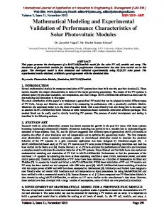
The goal of this section is to model the thin-layer structure (polarized in the main field) as a distribution of dipoles, the field of which is the superposition of fields due to all the dipoles representing the thin-layer structure. In our interpretation of the magnetic thin-layer modeling, we have started with a magnetic dipole moment of a current loop description (Figure 1). Let the current loop 𝐿 with current 𝐼 be positioned in a plane of the rectangular coordinate system [𝑥, 𝑦, 𝑧]. The magnetic field at the point 𝐵[𝑥0 , 𝑦0 , 𝑧0 ] determined by vector r can be expressed by a vector potential using curve or surface integral form [11, 12]: A (r) =
z0
(4)
Figure 1: Theoretical configuration of the magnetic thin-layer sample positioned in a plane of the rectangular coordinate system [𝑥, 𝑦, 𝑧].
Theoretical configuration of the thin-layer sample positioning simulating the experimental laboratory arrangement is depicted in Figure 2. We suppose that the thin-layer sample is positioned in the 𝑥-𝑦 plane of the rectangular coordinate system [𝑥, 𝑦, 𝑧] and the thickness of the layer is neglected. According to Figure 2(a), the layer is limited by lengths of 2a and 2b, with the left-right symmetry. The magnetic field 𝐵0 of the NMR imager is parallel with the +𝑧-axis. The task is to calculate the 𝐵𝑧 (𝑥, 𝑦, 𝑧) component of the magnetic field in the point 𝐴[𝑥0 , 𝑦0 , 𝑧0 ]. Using general formula (4) for magnetic induction of the magnetic thin-layer calculation, respecting the experimental arrangement depicted in Figure 2, and assuming the position vectors: r = r1 − r2 ,
2 2 2 𝑟 = √(𝑥0 − 𝑥) + (𝑦0 − 𝑦) + (𝑧0 − 𝑧) , (5)
where r is a position vector and 𝐼 is a current equivalent to planar density of a dipole moment of the magnetic thin-layer, we can write the final formula in a double integral form as follows: 𝐵𝑧 (𝑥, 𝑦, 𝑧) =
𝜇0 𝐼 4𝜋 𝑎
𝑏
3−𝐼 𝑑𝑦]𝑑𝑥, × ∫ [∫ 2 2 2 3/2 −𝑎 −𝑏 [(𝑥 − 𝑥) +(𝑦 − 𝑦) +(𝑧 − 𝑧) ] 0 0 0 ] [ (6) where limits for integration are [−𝑎, 𝑎] and [−𝑏, 𝑏]. Numerical evaluation of (6) in an analytical form is relatively complicated. After integration, one obtains relatively huge and problematic expressions. To calculate the general resultant expressions in analytical and numerical forms and to obtain the final graphical interpretation of the 𝐵𝑧 (𝑥, 𝑦, 𝑧) components we used a simplified incremental calculation model using rectangular elements; see Figure 2(b).
Mathematical Problems in Engineering +z
B0
RF field
3 +y
+x
Oil slick
ds x0 −b
−tx
a
y0 r2
d
+y b
−a z0 r
tx
Water solution
an +x o
r1
−an
A[x0 , y0 , z0 ]
Oil slick image
Bz
Imaging plane (a)
(b)
Figure 2: (a) Theoretical configuration of the thin-layer sample positioned in the 𝑥-𝑦 plane. In calculations, the thickness of the layer and imaging planes was neglected. (b) Thin-layer sample (e.g., oil slick) positioned in the 𝑥-𝑦 plane of the rectangular coordinate system. Principles of incremental elements integration are indicated.
Imaging plane
30
20 y0
10
10
5
30
0 −40
20 10
−20
0 x0
20
0
y0
−40
0
40 (a)
(b)
−20
0 x0
20
40
(c)
Figure 3: Calculated magnetic field variations near the organic slick sample positioned in the 𝑥-𝑦 plane of the rectangular coordinate system, relative values. (a) 3D plot. (b) Contour plot. (c) Density plot.
For the final numerical calculation, the following simplifying condition was assumed: thickness of the layer being negligible and for the graphical interpretation of a rectangular magnetic thin-layer sample we assume the following relative values: 𝜇0 𝐼/4𝜋 = 1, position of the imaging plane 𝑧0 = 3.2, and dimensions of the magnetic thin-layer 𝑡𝑥 and −𝑡𝑥 were assigned proportionally to real slick thin-layer dimensions. The final simplified formula for incremental calculation using rectangular elements is in the form: 𝐵𝑧 (𝑥, 𝑦, 𝑧) +𝑛
= ∑∫
+𝑡𝑥
−𝑛 −𝑡𝑥
±𝑎𝑛 ±𝑑
[∫ [
±𝑎𝑛
3−𝐼 2
2
2 3/2
[(𝑥0 − 𝑥𝑡 ) + (𝑦0 − 𝑦𝑛 ) + (𝑧0 ) ]
𝑑𝑦]𝑑𝑥. ] (7)
The resultant 3D and 2D plots of relative values of magnetic field for {𝑥0 , −40, 40} and {𝑦0 , −4, 36} are depicted in Figure 3.
The experimental results confirmed that the density plot representation corresponds best with the obtained MR image; see Figure 3(c).
3. Experimental Results For experimental evaluation of the mathematical modeling, we have chosen a simple laboratory arrangement by application of the magnetic resonance imaging methods. For sample positioning, a plastic vessel was used (Figure 4). A very thin isolating plastic membrane, separating the sample from the liquid, was placed at its bottom. The height of liquid level could be up to 10 mm. A special liquid solution was used to shorten the measuring time of the imaging sequence gradient echo and to speed up the data collection [8, 9]. The liquid contained 5 mM NiCl2 + 55 mM NaCl in distilled water. This solution enabled to shorten
4
Mathematical Problems in Engineering
RF coil
Liquid level
Imaging plane
B0 RF field +z
+y Plastic vessel
Sample position
Figure 4: For sample positioning, a plastic holder was constructed. Static magnetic field of the imager 𝐵0 is perpendicular and RF field is parallel to the plane of the holder.
the repetition time TR of the imaging sequence due to its reduction of H2 O relaxation time 𝑇1 . A special solenoidal RF transducing coil was constructed and placed near the sample. The plastic vessel and the RF coil together with a sample were placed into the centre of a permanent magnet of the imager. Imaging plane is perpendicular to the orientation of the static magnetic field (𝐵0 ). The next series of pictures shows theoretical and experimental results with imaging of magnetic field variations near the very thin soft magnetic materials detected by the magnetic resonance imaging method using carefully tailored GRE measuring sequences [10]. As a physical object, oil slick (dimensions 75×60 mm) was used. For comparison, a soft magnetic sample cut from a data disc, thickness 80 𝜇m, and a thin copper wire formed in the shape of an oil slick were used. Results by magnetic resonance imaging are visible in Figure 5. The second part of our experiments was aimed at the thin circularly shaped weak magnetic layers. For theoretical calculations, the formula (7) was applied where incremental elements for integration respected the circular shapes. The resultant image was calculated as a difference of a larger and a smaller circle (Figure 6). Next experiments were oriented to imaging of weak magnetic materials—plastic circular magnetic disks. Figure 7(a) represents the original diskette used for data storing and separated circular magnetic disc inserted to the holder used for imaging (Figure 7(b)). Resultant images show the original diskette with visible data sectors and the same diskette after application of DC and AC magnetic fields (Figure 8).
4. Discussion and Conclusion A modified method for mapping and imaging of the planar organic samples and weak magnetic inorganic samples placed into the homogenous magnetic field of an NMR imager was proposed. First experiments showed the suitability of the method even in the low-field MRI (0.2 Tesla). The goal of this study was to propose an MRI method used for soft magnetic material detection. Computation of the magnetic field variations based on thin-layer magnetic theory showed acceptable correspondence of theoretical results with experimental images. Mathematical analysis of an oil slick and weak magnetic object, representing a shaped magnetic thin-layer, showed
(a)
(b)
(c)
Figure 5: (a) Image of the oil slick, GRE imaging sequence, TR = 800 ms, TE = 10 ms, and slice thickness 2 mm. (b) Image of the soft magnetic sample, GRE, TR = 400 ms, TE = 10 ms, and slice thickness 2 mm. (c) Image of the thin coil wired up to the oil slick shape, DC current 20 mA, GRE, TR = 500 ms, and TE = 10 ms.
theoretical possibilities to calculate magnetic field around any type of samples. Calculated 3D images showed expected shapes of the magnetic field in the vicinity of the thinlayer samples. Density plot images showed magnetic field variations caused by samples placed into the homogeneous magnetic field of the NMR tomograph, which is very similar to the images gained by magnetic resonance imaging using a GRE measuring sequence.
Mathematical Problems in Engineering
5
4
2 10
y0 0 5
5 −2 0 −5
0
y0
−4
0
−4
x0
0 x0
−2
5 −5 (a)
2
4
(b)
Figure 6: Calculated magnetic field of a small plastic circular magnetic disk used to store data or programs for a computer—sample placed in the 𝑥-𝑦 plane. Incremental calculation method was used. (a) 3D plot. (b) Density plot. y
∅2
x ∅1
(a)
(b)
Figure 7: (a) Verbatim DataLife MF 2HD 3.5 Diskette to store data or programs for a computer, in original packing, dimensions 90 × 93 × 3.2 mm. (b) Plastic circular magnetic disk separated from the diskette case, diameters: 01 = 25 mm, 02 = 85 mm, and thickness 0.08 mm.
(a)
(b)
(c)
Figure 8: Images of the diskette: (a) original diskette with visible sectors, (b) diskette with 2 larger and 4 smaller stains caused by 1-second magnetization bringing closer small circular neodymium magnets 1 Tesla, and (c) diskette demagnetized by 50 Hz demagnetizer with 10 mm linear slot. Experimental imaging parameters: GRE, TR = 400 ms, TE = 10 ms, and slice thickness 2 mm.
6 The experiments prove that it is possible to map the magnetic field variations and to image the specific structures of thin samples using a special plastic holder. The shapes of experimental images, Figure 5, correspond to the real shapes of the samples. Some of the resultant images are encircled by narrow stripes that optically extend the width of the sample. This phenomenon is typical for susceptibility imaging, when one needs to measure local magnetic field variations representing sample properties [10, 12]. The experimental results are in good correlation with the mathematical simulations. This validates the possible suitability of the proposed method for detection of selected thin-layer organic and weak magnetic materials using the MRI methods. Presented images of thin objects indicate the potential of this methodology even in low-field MRI. The proposed method could be used in a variety of imaging experiments, for example, on very silky samples, textile material treated by magnetic nanoparticles, biological samples, documents equipped with hidden magnetic domain, magnetic tapes, credit cards and travel tickets with magnetic strips, banknotes, polymer fibers treated by a solution of nanoparticles in the water used in surgery, and more.
Acknowledgments This work was financially supported by the Grant Agency of the SAS, Project no. VEGA 2/0090/11 and by the project: Competence Center for New Materials, Advanced Technologies and Energy ITMS 26240220073 and Operational Program funded by the European Regional Development Fund. The mathematical model and measured data were processed using the program package Mathematica (Wolfram Research Inc., Champaign, IL, USA).
References [1] G. Wentzel, “Comments on Dirac’s theory of magnetic monopoles,” Progress of Theoretical Physics Supplement, vol. 3738, pp. 163–174, 1966. [2] J. A. C. Bland and B. Heinrich, Ultrathin Magnetic Structures III: Fundamentals of Nanomagnetism, Springer, Berlin, Germany, 2005. [3] O. Mosendz, G. Woltersdorf, B. Kardasz, B. Heinrich, and C. H. Back, “Magnetization dynamics in the presence of pure spin currents in magnetic single and double layers in spin ballistic and diffusive regimes,” Physical Review B, vol. 79, no. 22, Article ID 224412, 10 pages, 2009. [4] N. M¨usgens, E. Maynicke, M. Weidenbach et al., “Currentinduced magnetization dynamics in single and double layer magnetic nanopillars grown by molecular beam epitaxy,” Journal of Physics D, vol. 41, no. 16, Article ID 164011, 5 pages, 2008. [5] E. M. Haacke, M. Makki, Y. Ge et al., “Characterizing iron deposition in multiple sclerosis lesions using susceptibility weighted imaging,” Journal of Magnetic Resonance Imaging, vol. 29, no. 3, pp. 537–544, 2009. [6] I. Frollo, P. Andris, J. Pˇribil, and V. Jur´aˇs, “Indirect susceptibility mapping of thin-layer samples using nuclear magnetic resonance imaging,” IEEE Transactions on Magnetics, vol. 43, no. 8, pp. 3363–3367, 2007.
Mathematical Problems in Engineering [7] P. T. Callaghan and J. Stepisnik, “Spatially-distributed pulsed gradient spin echo NMR using single-wire proximity,” Physical Review Letters, vol. 75, no. 24, pp. 4532–4535, 1995. [8] M. Sekino, T. Matsumoto, K. Yamaguchi, N. Iriguchi, and S. Ueno, “A method for NMR imaging of a magnetic field generated by electric current,” IEEE Transactions on Magnetics, vol. 40, no. 4, pp. 2188–2190, 2004. [9] O. Strbak, P. Kopcansky, M. Timko, and I. Frollo, “Single biogenic magnetite nanoparticle physical characteristics. A biological impact study,” IEEE Transactions on Magnetics, vol. 49, pp. 457–462, 2013. [10] E. M. Haacke, R. W. Brown, M. R. Thompson, and R. Venkatesan, “Magnetic properties of tissues: theory and measurement,” in Magnetic Resonance Imaging: Physical Principles and Sequence Design, chapter 25, pp. 741–779, Wiley-Liss, John Wiley and Sons, New York, NY, USA, 1st edition, 1999. [11] J. D. Kraus and D. A. Fleisch, Electromagnetics with Applications, chapter 1, 2, McGraw-Hill, 5th edition, 1998. [12] J. Jianming, Electromagnetic Analysis and Design in Magnetic Resonance Imaging, M. R. Neuman, Ed., Biomedical Engineering Series, CRC Press, 1999. [13] G. Retter, Magnetische Felder und Kreise, chapter 2, VEB Deutscher Verlag der Wissenschaften, Berlin, Germany, 1961. [14] J. D. Jackson, Classical Electrodynamicsedition, John Wiley & Sons, New York, NY, USA, 3rd edition, 1998. [15] Textbook of Physics, Charles University in Prague, Faculty of Mathematics and Physics, http://physics.mff.cuni.cz/ kfpp/skripta/kurz fyziky pro DS/www/fyzika.
Advances in
Operations Research Hindawi Publishing Corporation http://www.hindawi.com
Volume 2014
Advances in
Decision Sciences Hindawi Publishing Corporation http://www.hindawi.com
Volume 2014
Journal of
Applied Mathematics
Algebra
Hindawi Publishing Corporation http://www.hindawi.com
Hindawi Publishing Corporation http://www.hindawi.com
Volume 2014
Journal of
Probability and Statistics Volume 2014
The Scientific World Journal Hindawi Publishing Corporation http://www.hindawi.com
Hindawi Publishing Corporation http://www.hindawi.com
Volume 2014
International Journal of
Differential Equations Hindawi Publishing Corporation http://www.hindawi.com
Volume 2014
Volume 2014
Submit your manuscripts at http://www.hindawi.com International Journal of
Advances in
Combinatorics Hindawi Publishing Corporation http://www.hindawi.com
Mathematical Physics Hindawi Publishing Corporation http://www.hindawi.com
Volume 2014
Journal of
Complex Analysis Hindawi Publishing Corporation http://www.hindawi.com
Volume 2014
International Journal of Mathematics and Mathematical Sciences
Mathematical Problems in Engineering
Journal of
Mathematics Hindawi Publishing Corporation http://www.hindawi.com
Volume 2014
Hindawi Publishing Corporation http://www.hindawi.com
Volume 2014
Volume 2014
Hindawi Publishing Corporation http://www.hindawi.com
Volume 2014
Discrete Mathematics
Journal of
Volume 2014
Hindawi Publishing Corporation http://www.hindawi.com
Discrete Dynamics in Nature and Society
Journal of
Function Spaces Hindawi Publishing Corporation http://www.hindawi.com
Abstract and Applied Analysis
Volume 2014
Hindawi Publishing Corporation http://www.hindawi.com
Volume 2014
Hindawi Publishing Corporation http://www.hindawi.com
Volume 2014
International Journal of
Journal of
Stochastic Analysis
Optimization
Hindawi Publishing Corporation http://www.hindawi.com
Hindawi Publishing Corporation http://www.hindawi.com
Volume 2014
Volume 2014