a way that no one apart from the sender and intended recipient suspects the existence of the message. ... email-spams can be used as cover objects. Whereas ... Steganalysis is the process of identifying stego-objects from the bulk of innocent ...
IOSR Journal of Computer Engineering (IOSRJCE) ISSN: 2278-0661 Volume 2, Issue 5 (July-Aug. 2012), PP 01-15 www.iosrjournals.org
Mathematical Modeling of Image Steganographic System Kaustubh Choudhary Scientist, Defence Research and Development Organisation (DRDO), Naval College of Engineering, Indian Naval Ship Shivaji,Lonavla, Maharashtra, India
Abstract: Image based steganography is a dangerous technique of hiding secret messages in the image in such a way that no one apart from the sender and intended recipient suspects the existence of the message. It is based on invisible communication and this technique strives to hide the very presence of the message itself from the observer. As a result it becomes the most preferred tool to be used by Intelligence Agencies, Terrorist Networks and criminal organizations for securely broadcasting, dead-dropping and communicating information over the internet by hiding secret information in the images. In this paper a mathematical model is designed for representing any such image based steganographic system. This mathematical model of any stego system can be used for determining vulnerabilities in the stego system as well as for steganalysing the stego images using same vulnerabilities. Based on these mathematical foundations three steganographic systems are evaluated for their strengths and vulnerabilities using MATLAB ©Image Processing Tool Box. Key Words: Cyber Crime, Global Terrorism, Image Steganography, LSB Insertion, Mathematical Model of Image Steganographic System
I.
Introduction
Steganography is the art and science of writing hidden messages in such a way that no one, apart from the sender and intended recipient suspects the existence of the message. It is based on invisible communication and this technique strives to hide the very presence of the message itself from the observer. Herodotus‟s Histories describes the earliest type of stegenography. It states that “The slave’s head was shaved and then a Tattoo was inscribed on the scalp. When the slave’s hair had grown back over the hidden tattoo, the slave was sent to the receiver. The recipient once again shaved the slave’s head and retrieved the message”. All steganographic techniques use Cover-Object and the Stego-Object. Cover-object refers to the object used as the carrier to embed the messages into it. In the above example the slave‟s head (without tattoo) is the cover object. In modern context Images, file systems, audio, video, HTML pages, word documents and even email-spams can be used as cover objects. Whereas stego-object is the one which is carrying the hidden message. I.e. in the above example the „slaves head with fully grown hair and a hidden tattoo‟ is acting as the stego-object. Contemporary Steganography can be of various types depending upon the nature of the cover object and the method used for hiding information in that cover object. This technique is frequently used in espionage, organized crime and is especially popular among terrorist networks. Among all those steganographic techniques the digital Image based steganography is most commonly used due to numerous advantages offered by it.[1] But the most important advantage is substantial difficulty in steganlysis of the digital image. Steganalysis is the process of identifying stego-objects from the bulk of innocent objects and further extracting the hidden information from the same. The identification of the steganographic signature in the innocent looking stego-image is the most difficult part of any steganalysis algorithm. Once this malicious stego-image is identified then either the hidden data can be extracted from it or the data in it can be destroyed or can be even used for embedding counter-information in the same Digital image consists of numerous discrete pixels. Any pixel P(x,y) located at xth row and yth column of the image has a particular color which is combination of the intensity levels of three primary colours Red, Green and Blue and jointly called as RGB value of the pixel P(x,y). For example in a 24 bit BMP image RGB values consists of three 8 bits for each R,G and B and thus a pixel is a combination of 256 different shades (ranging from intensity level of 0 to 255) of red, green and blue resulting in 256 x 256 x 256 or more than 16million colors. Thus if the least significant bits in the R, G and B value are changed the pixel will have minimal degradation of 2/256 or 0.78125%.This minor degradation is psycho-visually imperceptible to us due to limitations in Human Visual System (HVS). But at the cost of this negligible degradation 3 bits (1 bits each from red, green and blue) are extracted out of every pixel for transmitting our secret information. The most of the Spatial Domain Image steganographic techniques use this method of LSB Insertion for hiding data in the image. There are other techniques also for hiding data in the image. For example Transformation Domain Steganography may use Discrete Cosine Transforms or Discrete Wavelet Transform for embedding data and some other steganographic algorithm may use a different color space itself (Example RGB may be converted to YCbCr and then various steganographic techniques can applied).
www.iosrjournals.org
1 | Page
Mathematical Modeling Of Image Steganographic System In this paper a Universal mathematical model is designed for representing any Image Based Steganographic System unambiguously as a mathematical structure. Based on this mathematical model three Spatial Domain Transformation based LSB Insertion algorithms are evaluated for susceptibility to steganalysis.
II.
Mathematical Model of Image Steganography System
Any steganographic algorithm or simply Stego-algorithm is composed of Stego-Function Ғ and inverse of Stego-Function Ғ-1. Ғ takes Cover-Image C and Information I as input and generates Stego-Image S as the output. At the receiver end the Stego-Image S is fed to decoding algorithm which is mathematically inverse of Stego-Function Ғ(represented as Ғ-1) and produces Information I. These two function along with the entire set of their domain and co-domain form the Steganographic System Ψ (or simply Stego-system). Mathematically this can be represented as S = Ғ(C, I) and I = Ғ-1(S) and Ψ = {Ғ, Ғ-1, C, S, I}. 2.1 Universal Stego System: A perfect Depicter of a Stego-Algorithm A same stego-algorithm may operate on different cover images and may insert different informations in them. So any stego system Ψ = {Ғ, Ғ-1, C, S, I} is different for every pair of cover image C and Information I even though the Algorithm of Stego- system Ψ given as Ψ(Algorithm) = { Ғ, Ғ-1} remains the same for all those pairs. So we introduce the concept of Universal Stego System which is Universal Set of all stego systems Ψ = {Ғ, Ғ-1, C, S, I} which have same Stego-Algorithm Ψ(Algorithm) = { Ғ, Ғ-1}.We represent any Universal Stego System by Φ ={ Ғ, Ғ-1, ℂ , 𝕊, 𝕝 } where is set of all cover Images, 𝕊 is set of all stego-images and 𝕝 is set of all Information and stego algorithm of Φ given as Φ(Algorithm) = { Ғ, Ғ-1}. Thus any stego system Ψ = {Ғ, Ғ-1, C, S, I} is an instance of stego algorithm { Ғ, Ғ-1} or Universal Stego System Φ ={Ғ, Ғ-1, ℂ , 𝕊, 𝕝 }. Mathematically we represent a Universal Stego System Φ as:
(1) 2.2 Security of Stego Algorithm Susceptibility to steganalysis of any stego algorithm depends upon its Security. As pointed by Cachin in his Information theoretic model [2] and Zollner et.al in Modeling the security of steganographic systems [3] the stego-algorithm {Ғ, Ғ-1} ∈ Φ is said to be ε-secure (ε ≥ 0) if the relative entropy (given by H(Pc||Ps)) between the probability distributions (Probability Mass Function) of cover-image C ∈ ℂ and the stego-image S ∈ 𝕊 given as Pc and Ps respectively is at most ε for every C , S and I in Φ. The security of Stego Algorithm {Ғ, Ғ -1} ∈ Φ is same as security of Universal Stego System Φ and are represented as {Ғ, Ғ-1}(α) or Φ(α) respectively. Therefore {Ғ, Ғ-1}(α) and Φ(α) are one and the same.
(2) The security of any Stego-System Ψ = {Ғ, Ғ-1, C, S, I} is given as Ψ(α) and is secure (that is Ψ(α) = ) if H(Pc||Ps) = . But this has very narrow connotation as Stego-Algorithm {Ғ, Ғ-1} has to operate not just on C, S and I but on every C ∈ ℂ , every S ∈ 𝕊 and every I 𝕝. But still the concept of security of any StegoSystem Ψ = {Ғ, Ғ-1, C, S, I}forms the basic building block of the concept of security of any Stego-Algorithm { Ғ, Ғ-1} in Universal Stego System Φ = { Ғ, Ғ-1, ℂ , 𝕊, 𝕝 }. This is because any stego algorithm {Ғ, Ғ-1} Φ is secure (ie {Ғ, Ғ-1}(α) or Φ(α) = ) then maximum value of security of any Stego-System Ψ ∈ Φ (given as Ψ(α)) can be for some Ψ ∈ Φ. Mathematically this can be written as: (3) Thus the security of Stego Algorithm {Ғ, Ғ-1} or Universal Stego System Φ is defined in terms of Stego System Ψi ∈ Φ. According to Cachin a stego-system is perfectly secure if H(Pc| Ps = 0, which is www.iosrjournals.org
2 | Page
Mathematical Modeling Of Image Steganographic System possible only when Pc = Ps and in such cases receiver is unable to distinguish between C and S as their probability distributions are same and this represents the Shannon‟s notion of perfect secrecy for cryptosystems[4]. However Chandramouli et.al in Steganography Capacity: A Steganalysis Perspective [4] have pointed that this definition of Security of stego-system is purely theoretical in nature because it assumes the Cover-object C to be perfectly random. But in reality the Image is not random and in some cases it is possible to steganalyse the image even if the probability distributions of the C and S are same. Hence in addition to parameter some more parameters of security of any Universal stego system are devised. 2.2 Preliminaries and Definition Using Cachin‟s Information theoretic model[3] and Chandramouli‟s Mathematical formulation of a Steganalytic Problem[6] and extending both to Image based stego-system a method is devised for representing this system mathematically. Based on this mathematical model a technique is devised for steganlaysis of the stego image. Before we proceed to mathematical model of Image based stego-system we have to mathematically define the preliminary concepts to be used in this model. Definition 1 (Image) Every digital image is collection of discrete picture elements or pixels. Let M be any digital image with N pixels. So any particular pixel of image M is represented as M(z) and z can be any value from 1 to N. This M(z) can be a gray level intensity of the pixel in gray scale image or RGB or YCbCr value of the pixel in a color Image. Thus M(z) can be a set {R(z),G(z),B(z)} or equivalent gray scale representation or (R(z)+G(z)+B(z))/3. But it is always better to consider each R, G and B components individually because the averaging effect cause loss of vital steganographic information. Further < {M},m > is multiset of Image M such that M(z) ∈ {M} for every z = 1 to N and m is a vector corresponding to the occurrence or count of every element M(z) in {M}. Mathematically an image M with N pixels is:
(4) Definition 2 (Identical Images) Two images M and L with N pixels are said to be identical (represented as M ≡ L) if they have pixel to pixel match. This means that two images are identical and absolutely same. Thus their difference image D = ML will be a pure black image corresponding to zero matrix. (5) Definition 3 (Probability distribution of Image) Probability distribution or Probability Mass Function represented as P(M) for image M = < {M},m > is 𝑚 a multiset where m‟ = and n(< {M}, m >) is cardinality (number of elements) of n()
multiset of the image M or simply total number of pixels in M. The same is explained mathematically in (6).
(6) Definition 4 (Macro statistically Same Images) Two images M and L with N pixels are said to be Macro Statistically Same (represented as M L) if they have equal entropy, energy, contrast ratio, brightness and same histograms. However this does not mean that they are having pixel to pixel match and may not be identical. It simply means that the probability distributions of their pixels are equal. Thus if M L then = or in terms of probability distribution P(M) = P(L). In other words images M and L will have same number of occurrence of any certain pixel intensity but it is not necessary that M(z) = N(z) for any particular z from 1 to N in the image. Thus
(7) Definition 5 (Neighborhood or Locality of Pixel) If ℓ(M(z)) is said to be set of neighboring pixels of any pixel M(z) in image M. Then any n i ∈ ℓ(M(z)) will be such that d(ni , M(z) ) ≤ λ where d is a function which calculates distance (can be Euclidean, City-Block, www.iosrjournals.org
3 | Page
Mathematical Modeling Of Image Steganographic System Chess Board or any other type depending upon the steganographic algorithm) between its inputs (ie n i and M(z)) and λ is measurement of degree of neighbourhood and should be minimum (Generally equal to 1 pixel) but also depends upon the steganographic algorithm used by stegosystem Ψ. Mathematically this can be represented as: (8) In Fig 1 an arbitrary pixel Y is shown with its neighbors P, Q, R, S, T, U, V and W. We represent this pixel Y as Y in mathematical notation. Thus ℓ(Y) = {P, Q, R, S, T, U, V ,W} is set of neighboring pixels of pixel Y. Here λ = 1 and distance function d calculates Chess Board Distance. P S U
Q Y V
R T W
Fig 1 Pixel Y Definition 6 (Adjacent Neighbors of Pixel) Set of Adjacent Neighbors of a pixel M(z) is given as 𝒜 (M(z)). Thus 𝒜 (M(z)) is a collection of set {M(x), M(y)} such that M(x) ∈ ℓ(M(z)) and M(y) ∈ ℓ(M(z)) and they are adjacent i.e d (M(x) , M(y)) = 1 where d is a function which calculates distance. Mathematically:
(9) In Fig 1 for an arbitrary pixel Y with ℓ(Y) = {P, Q, R, S, T, U, V ,W} the 𝒜(Y) = {{P,Q}, {Q,R)}, {R,T}, {T,W}, {W,V},{V,U},{U,S},{S,P}}. Definition 7 (Pixel Aberration) Pixel Aberration of any Pixel M(z) from its neighborhood ℓ(M(z)) in terms of Standard Deviation of ℓ(M(z)) is given as 𝛿 ( M(z) , ℓ(M(z))). It is a quantifier which gives the idea of the amount of deviation of the pixel from its neighborhood. In any natural image a pixel M(z) is expected to be as much different from its neighborhood as the adjacent pixels in ℓ(M(z)) themselves are. For any pixel M(z) the mean of its absolute difference from its neighborhood ℓ(M(z)) is given as (𝑀 𝑧 , ℓ 𝑀 𝑧 ). And the set representing the absolute differences of the adjacent neighbors of M(z) among themselves is given as 𝒟(𝒜 (M(z))). The mean of the values of 𝒟(𝒜 (M(z))) is given as 𝐷(𝐴 (𝑀(𝑧))) and Standard Deviation of the values of 𝒟(𝒜 (M(z))) is given as 𝜎(𝒟(𝒜 (M(z)))) . Since M(z) is also a immediate neighbor of ℓ(M(z)) so (𝑀(𝑧), 𝑙(𝑀(𝑧) )) must be within the limits of standard deviation of 𝒟(𝒜 (M(z))) and mean of 𝒟(𝒜 (M(z))). This degree of deviation of M(z) from its neighbors ℓ(M(z)) in terms of 𝜎(𝒟(𝒜 (M(z)))) and 𝐷(𝐴 (𝑀(𝑧))) is quantified as 𝛿 ( M(z) , ℓ(M(z))) and hence it represents the aberration in the pixel M(z). In terms of Fig 1 the mean of the differences of pixel Y with its neighbors i.e. elements of ℓ(Y) is given as Y-P,Y-Q, Y-R, Y-S, Y-T, Y-U, Y-V and Y-W and should be close to the differences of the adjacent pixels in ℓ(Y) i.e. difference of the elements of {P,Q},{Q,R)},{R,T},{T,W}{W,V},{V,U},{U,S} and {S,P} or simply PQ, Q-R, R-T, T-W, W-V,
V-U, U-S and S-P. Thus (𝑀 Y , ℓ 𝑀 Y ) is mean of modulus of Y-P, Y-Q, Y-R,
Y-S, Y-T, Y-U, Y-V and Y-W and 𝒟(𝒜 (Y)) = {modulus of P-Q, Q-R, R-T, T-W, W-V, V-U, U-S and S-P}. So aberration in pixel Y with respect to its neighborhood ℓ(Y) given as 𝛿 ( Y , ℓ(Y)) should be within the limits of standard deviation of 𝒟(𝒜(Y)) and 𝐷(𝐴(𝑌 ̇)) . Mathematically:
(10) Definition 8 (Pixel Aberration of Image) In any image M with N pixels the Pixel aberration of image M is given as 𝛿(𝑀). It is the weighted mean of the modulus of the pixel aberrations of the pixels of the entire image M. Since for any image M the 𝛿 M z ,ℓ M z is the measure of deviation of M(z) from its neighborhood ℓ M z in terms of standard www.iosrjournals.org
4 | Page
Mathematical Modeling Of Image Steganographic System deviation so majority of pixels have this values located close to zero and approximately more than 68% of the pixels have pixel aberration within 1 ( as per 3 Sigma or 68-95-99.7 rule of Statistics). Hence the simple mean of 𝛿 M z , ℓ m z is very close to zero and is insignificantly small for all images. Since by pixel aberration analysis we have to identify those images which have larger pixel aberrations so as a remedy very small weights are assigned to less deviated values (majority of pixels which have low pixel aberration values) and larger weights are assigned to more deviated values (few counted pixels have large pixel aberrations). Thus value of 𝛿(𝑀) for the Image M with N pixels is given as:
(11) The weight W(z) for the pixel M(z) is much smaller for small values of 𝛿 M z , ℓ m z
and quite
large for big values of 𝛿 M z , ℓ m z . Thus W(z) is large for pixel having greater pixel aberration and very small for pixels having lesser pixel aberration. Such weights can be computed by taking cube of the value of pixel aberration in terms of the standard deviation. In other words the weight W(z) for any Pixel M(z) in image M is given as W(z) =
𝛿 M z ,ℓ M z
– MEAN ZZ =N =1 (𝛿 M z ,ℓ M z
STD ZZ =N =1 (𝛿 M z ,ℓ M z
)
3
)
(12) Although we may avoid taking weighted mean and we can use simple mean but for that we have to consider only those values of 𝛿 M z , ℓ M z for determining mean which are above or below certain threshold ± 𝝉 and rest of the values can be filtered. This value of 𝝉 is generally given in terms of standard deviation of 𝛿 M z , ℓ M z from z = 1 to N and in represented as τ. Thus Mean Pixel Aberration of Image M at threshold 𝛕 is represented as 𝜹 𝑴, 𝛕 and mathematically defined as:
(13) Thus this value of depends on smoothness of the cover image and the type of aberration we are interested in. In unsmooth cover images the differences of the pixels with their neighbors is quite large (for example an image of a Forest or Valley) and hence the value of 𝛿 𝑀, τ at larger represents the mean of only those deviations which are larger than τ. Whereas for smooth cover images like clear blue sky the aberration is already very low and hence smaller value of produces good result. Definition 9 (Range of Pixel Aberration in the Image) In any image M with N pixels the Range of Pixel aberration of image M is given as ℛ(𝑀). It is the difference of the Maximum Pixel Aberration (ℛ 𝑀 ↑ in the image M and Minimum Pixel Aberration (ℛ 𝑀 ↓ in the Image M. Thus Mathematically the same can be expressed as:
(14) Definition 10 (Maximum Deviation in the Pixel Aberration of the Image)
www.iosrjournals.org
5 | Page
Mathematical Modeling Of Image Steganographic System In any image M with N pixels the Maximum Pixel Aberration in M given as (M) is the maximum pixel aberration in absolute terms in the image M. τ corresponding to (M) is represented as 𝒯. Thus (15)
(16) 2.3 Detailed Mathematical Model of any Image based Stego Algorithm In Equation 2 it has been very clearly shown that security of any stego system Ψ = {Ғ, Ғ-1, C, S, I} is the basic building block of security of the stego-algorithm {Ғ, Ғ-1}. So for the sake of simplicity it is better to operate on stego-system only. Let Ψ = {Ғ, Ғ-1, C, S, I} be any Image Steganographic System with Ғ, Ғ-1, C, S and I having the same meaning as mentioned in previous section. Thus S = Ғ (C, I) and I = Ғ-1(S) also holds well. Now let us assume that Cover Image C consists of N discrete pixels represented by C(1), C(2), … C(N). Although cover image C is meant for storing Information I. But any arbitrary pixel C(z) of C can at max store only a limited part of Information I. Let this small part of I stored in C(z) be represented as I(z). Thus our Information I can be broken to K parts represented by I(1), I(2) …I(K), K ≤ N such that any I(z) is the information stored in any particular pixel C(z) for any z ≤ N. If information I is smaller than the cover-image C ie if K < N then the remaining I(z) from z = K+1 to N can be thought to be empty or Null set and given as I(z) = { } for z = K+1 to N. Thus the cardinality of both I and C (given as n(I) and n(C) respectively) is made equal i.e. N. Since S = Ғ (C, I) so corresponding to every C(z) in C we have a unique S(z) in S. Using the notations of Set Theory the same is mathematically written in (17).
(17) The stego-function Ғ:(C, I) → S can be redefined at pixel level as S(z) = α(z) [C(z) ● I(z)] where ● is any operator used by stego-funtion Ғ acting over C and I to produce S and α(z) ≥ 0 is factor which strengthens Ψ for z = 1 to N. Thus α(z) ∀z: 1≤ z ≤ N is strengthening factor of stego system Ψ and helps it in achieving secure Ψ (ie α(z) for z = 1 to N is the factor which helps in achieving Ψ(α)). The inverse stego function Ғ-1 :(S) → I can be redefined at pixel level as I(z) = Θ (S(z)) where Θ is a unary operator used by Ғ-1 acting on S to produce I and hence indirectly C also. Thus algorithmically unary operator Θ is inverse of the operator ●. 2.3.1 Parameters for Measuring Strength of Stego Algorithm Strengthening Factor α(z) ∀z: 1≤ z ≤ N, keeps S(z) such that it is least susceptible to any steganalysis attacks by making S perfectly resemble an Innocent Image i.e. without any distortions. Therefore this α(z) has to meet four main requirements which are explained next. Requirement 1 Using operator ● the α(z) should map C(z) and I(z) to S(z) in such a way that relative entropy of cover and stego image given as H(P(C) || P(S)) should be minimum possible. Here P(C) is probability distribution of C and P(S) is probability distribution (Probability Mass Function) of S and H(P(C) || P(S)) is relative entropy of P(C) with P(S). This requirement is derived from equation 1 mentioned in section 2.2. This simply means that macro statistical parameters of the Cover-Image C and Stego-Image S should be almost same or in terms of relative entropy should be minimum possible. This requirement is extension of Cachin‟s Information theoretic model in terms of α. Mathematically this can be expressed as α(z) should be such that:
(18) www.iosrjournals.org
6 | Page
Mathematical Modeling Of Image Steganographic System Where P(C) and P(S) are probability distribution of C(z) and S(z) ∀z: 1≤ z ≤ N and such a stegosystem is said to be ε Secure. In order to achieve this requirement the stego function Ғ:(C, I) → S will macro-statistically redistribute the pixels of C in such a way that even though corresponding pixels C(z) and S(z) may not be same but still probability distribution of pixels C(z) in C and S(z) in S for z = 1 to N will remain same that is C S will be achieved. Thus by fulfilling this requirement (assuming ε = 0) the Cover Image and the Stego Image will have same Histogram, Brightness, entropy, energy, contrast ratio and all other macro statistical parameters even if C S that is C(z) ≠ S(z) ∀z:1≤ z ≤ N. Requirement 2 If only Requirement 1 is met we may have a situation where even though the cover-image may look macro-statistically same (in terms of Histogram, Brightness, entropy, energy, contrast ratio etc) as stego-image but still they may have significantly different pixel to pixel correspondence between C and S. I.e. any particular pixel S(z) of S may be considerably different from C(z) of C thus revealing the distortions in S(z) and hence making S susceptible to Steganalysis. Thus in addition to macro-statistical redistribution of the pixels of cover image (as mentioned in Requirement 1) the stego-algorithm must redistribute the pixels of the neighborhood of every pixel C(z) in C (i.e. ∀z: 1≤ z ≤ N) is such way that two corresponding pixels C(z) and S(z) should have same probability distribution of their neighborhood. Thus α(z) should meet another requirement: Using operator ● the α(z) should map C(z) and I(z) to S(z) in such a way that the relative entropy between the Neighborhood of C(z) and S(z) (or Local Relative Entropy) should be least possible ∀z: 1≤ z ≤ N. Thus any Image based Stego-System Ψ is said to be ξ Secure if the mean of the relative entropies of the neighborhood of C(z) and S(z) for all C(z) in C and S(z) in S (that is ∀z: 1≤ z ≤ N) is ξ. Thus α(z) should be such that ξ is minimum where is given as
(19) Here P ℓ(C z ) is probability distribution of the pixels in the neighbourhood of pixel C(z) and P(ℓ S z ) is probability distribution of the pixels in the neighbourhood of pixel S(z). Requirement 3 Most spatial domain Stego Algorithms distribute the entire information in large number of pixels and as a result the changes in the pixel values are very small and unnoticeable but in this process large number of the pixels in the image change and hence the relative entropy of the stego-image and cover-image increases due to considerable change in probability distribution of pixels in the image. Security of such algorithms can be defined by Requirement 1 and Requirement 2 that is ε and ξ. But there are certain Image Stego Algorithms which concentrate the information in very few pixels. As a result the change in pixels values of these few pixels is very large and hence quiet perceptible even though the probability distribution of pixels is not much disturbed. In case of such algorithms even if ε and are very small the stego-image may have few grains in last few rows (grains are due to large and perceptible changes in those few pixels and changes in the bottom most pixel usually goes unnoticed due to psycho-visual weaknesses of human eye) and are susceptible to steganalysis. In any natural Image a pixel P is almost same as its neighbors. Therefore on an average C(z) will not be very different from ℓ(C(z)) for most values in z = 1 to N. Thus α(z) should meet another requirement: Using operator ● the α(z) should map C(z) and I(z) to S(z) in such a way that any particular pixel should not change much. Thus the difference between Weighted Mean of the Pixel Aberration of Stego-Image S from Cover-Image C (Definition 8) should be minimum possible. The weighted mean pixel aberration 𝛿 can be calculated by either obtaining the Maximum of the red , green and blue values or by taking the average of red, green and blue values. Hence mathematically the difference between Weighted Mean of the Pixel Aberration of Stego-Image S from Cover-Image C is represented as 𝑒MAX and 𝑒MEAN and given as 𝒆MAX =MAXRGB( 𝜹 𝑺 ) − MAXRGB ( 𝜹 𝑪 ) or 𝒆MEAN =MEANRGB( 𝜹 𝑺 ) − MEANRGB ( 𝜹 𝑪 ) 20 The same can be alternatively represented by finding the difference between the mean pixel aberration of Cover Image C and Stego-Image S considering only those values of pixel aberrations (of δ C z , ℓ C z and δ S z , ℓ S z
for z = 1 to N) in entire image which are above a certain threshold ± 𝝉 and given www.iosrjournals.org
7 | Page
Mathematical Modeling Of Image Steganographic System as 𝛿 𝐶, τ and 𝛿 𝑆, τ Thus α(z) should be such that the difference between the pixel aberrations of Stego-Image and Cover-Image at threshold τ (in terms of standard deviation it corresponds to pixel aberration value of ± 𝝉) should be minimum possible and given as ℯ(τ). In unsmooth cover images the aberration is already very high and addition of information brings further more aberrations (in some efficient stego-algorithms it may reduce the aberrations too) so if the value of τ is kept large then ℯ(τ) will be measure of differences in only those large aberrations. Whereas in smooth cover images the aberration is quite low and hence lower value of is advisable. In some cases we may get a value of ℯ(τ) as negative which indicates that at threshold τ the Stego Image has lesser aberration then the cover image. Certain steganographic algorithms hide the data very efficiently and as a result only few counted pixels have aberration beyond the prescribed limit. In such cases determination of weaknesses in these algorithms using only fixed value ℯ(τ) goes unnoticed due to averaging effect of large number of pixels having much lower pixel aberration. Moreover ℯ(τ) has different value at every τ. Thus a better estimate of ℯ(τ) can be 𝑒 which is the mean of ℯ(τ) for continuously increasing value of τ from 0 to that value of τ which corresponds to modulus of Maximum Pixel Aberration (Definition 10) in the stego image that is for τ = 0 to 𝒯. 𝓮(𝛕) = 𝜹 𝑺, 𝛕 - 𝜹 𝑪, 𝛕
(21) 1
𝒯 = τ ∶ 𝝉 = ∆(M )
Since calculating the value of 𝑒 = 𝒯 0 ℯ τ 𝑑τ is practically very expensive in various accords of time and computation power. So more practical way to estimate of 𝑒 can be based on taking means of ℯ τ at any chosen discrete values of for example like = 0, 1/8 𝒯, 2/8 𝒯, 3/8 𝒯 ... 𝒯 . 1
𝒯 = τ ∶ 𝝉 = ∆(M)
Thus as an indicator of requirement 3 either 𝑒 = 𝛿 𝑆 − 𝛿 𝐶 or 𝑒 = 𝒯 0 ℯ τ 𝑑τ can be considered. But generally the difference of the weighted means of the pixel aberration of cover image and stego image as given as 𝑒 in (20) will be preferable although this may vary from algorithm to algorithm and situation to situation. Whatever the value we consider for obtaining this difference i.e. either 𝑒 or 𝑒 has to be represented by 𝑒 in the holistic representation of the requirement 4 in the steganographic system. Thus 𝑒 is either 𝑒 or 𝑒 . Requirement 4 Another very good indicator of presence of anomaly in the pixels of the image is Range of Pixel Aberration ℛ 𝑀 in the Image (Definition 9). Bigger value of ℛ 𝑀 in spite of lower values of ℯ(τ) indicates that only very few counted pixels have aberration much beyond the prescribed limit and hence the given image could be a potential stego-image. Thus using operator ● the α(z) should map C(z) and I(z) to S(z) in such a way that Range of Pixel Aberration in Cover Image must not be very different from the Range of Pixel Aberration in the Stego image. Thus the difference of Range of Pixel Aberration of Cover and Stego Image should be minimum possible and given as €.
(22) Thus € is the indicator of percentage change in the Range of Pixel Aberration in Cover Image after embedding the data in it. In colored Image the € value is different for Red, Green and Blue components of the Image. But we can‟t take average of the three as € value represents the Range of Pixel Aberration and hence for RGB image, this € is given as (23) Also it is better if we mention the color component which has maximum € in RGB Image. 2.4 Holistic Representation of Stego System and Universal Stego System Mathematically Based on these four requirements of α with regards to the Strength of any Steganographic System Ψ we may define security of Ψ by four tuple < ε, ξ, 𝑒, € > and say Ψ(α) = < ε, ξ, 𝑒, € > secure. Thus Image based Universal stego system Φ = { Ғ , Ғ-1, ℂ , 𝕊, 𝕝 } with any Stego System Ψ = {C, S, I, Ғ, Ғ1
} such that Ψ ∈ Φ can be more elaborately defined at pixel level as
www.iosrjournals.org
8 | Page
Mathematical Modeling Of Image Steganographic System
(24) Here Stego-Algorithm of Φ or Φ (Algorithm) = < ●, Θ > where Φ (Ғ) = ● and Φ (Ғ-1) = Θ and Strength of Φ given as Φ (α) = < ε, ξ, 𝑒, € >. Since handling of four different values of Φ(α) is quite difficult so four values of Φ (α) = < ε, ξ, 𝑒 , € > can be reduced in to one value represented as < Φ(α) > by taking weighted means of their modulus. (25) The values of these four weights w1 , w2 , w3 , w4 depends upon the alertness and sensitivity of steganalysis algorithm with respect to the four strength parameters ε, ξ, 𝑒, € of any steganographic algorithm. In most general cases we assume that the steganalyst is capable of exploiting any of these 4 vulnerabilities and therefore the four conditions have equal importance and hence w1 = w2 = w3 = w4 and therefore the value of < 𝛷 α > becomes simple mean of < ε, ξ, 𝑒, € > and given as < 𝛷 α > = (ε + ξ+ 𝑒 + € )/4. The smaller value of < 𝛷 α > indicates that the algorithm is stronger. Thus Image based Universal stego system Φ = { Ғ, Ғ-1, ℂ , 𝕊, 𝕝 } with any Stego System Ψ = {C, S, I, Ғ, Ғ-1} such that Ψ ∈ Φ can also be defined as
(26) 2.5 Steganalysis is Always Possible In this section a theorem is given which proves that every stego system is susceptible to steganalysis. Theorem: No Image based Stego Algorithm (Universal Stego System) is fool proof. Assumption Let there be any fool proof Universal stego system Φ = { , 𝕊, 𝕝 , Φ(Algorithm) , Φ(α)} such that Φ(α) = < ε, ξ, 𝑒, € > = < 0, 0, 0, 0 > and Φ(Algorithm) = { Ғ , Ғ-1} capable of exchanging Y distinct and authentic Information I1, I2 I3 … IY. Thus mathematically this assumption can be written as:
(27) Proof: Some information Ik∈ 𝕝 is being exchanged through above assumed Universal stego-system Φ using cover-image C ∈ of size N. As any IX ∈ 𝕝 is not empty ∀x: 1≤ x ≤ Y so Ik(z) ≠ { } for at least one z from 1 to N. As S(z) = α(z) [C(z) ● Ik(z)] and Φ(α) = < ε, ξ, 𝑒, € > = < 0, 0, 0, 0 > so S(z) will be such that S(z) = C(z) and hence Stego Image S and Cover Image C are identical or S ≡ C. Now a different Information Im ∈ 𝕝 is exchanged through same Universal Stego system Φ with same cover Image C. Again since S(z) = α(z) [C(z) ● Im (z)] and Φ(α) = < ε, ξ, 𝑒, € > = < 0, 0, 0, 0 > so S(z) = C(z). Therefore again S and C are identical or S ≡ C. Thus for any information Ix ∈ 𝕝 the Universal stego-system Φ is such that S and C are identical and same. But as we know that S = Ғ (C, I) and I = Ғ-1(S) so for every stego-image S there exists a unique Information I. But in the given case the same stego-image S corresponds to different distinct information I1, I2 I3 … IY. Hence we conclude that all information are same i.e. I1 = I2 = I3 = … = Ix = … = IY-1 = IY. But this is in contradiction with our assumption that {I1, I2 I3 … IY}∈ 𝕝 and I1≠ I2 ≠ I3 ≠ … ≠ IY. Thus our assumption is wrong and hence Φ(α) = < ε, ξ, 𝑒, € > ≠ < 0, 0, 0, 0 > and hence < Φ α > is more then 0. www.iosrjournals.org
9 | Page
III.
Mathematical Modeling Of Image Steganographic System Application of the Mathematical Model in Real Scenario for evaluation of Stego Algorithms
Based on the mathematical model developed in Section 2 three different spatial domain steganographic algorithms are evaluated for susceptibility to steganalysis. These three Algorithms are named as Algorithm I, Algorithm II and Algorithm III and represented mathematically as Universal Stego Systems Φ1, Φ2 and Φ3 respectively. These three steganographic algorithms were also used in [1] and are referred in Section 5 of [1] as Algorithm designed in section 4, QuickStego Software and Eureka Steganographer respectively. Thus Φ1(Algorithm) is Algorithm I, Φ2(Algorithm) is Algorithm II and Φ3(Algorithm) is Algorithm III. The features of these three algorithms are summarized in Table 1. For the sake of uniformity (which is required for Evaluation) we use same set of two different cover images for evaluation of Φ1, Φ2 and Φ3. One of them is smooth (has low Pixel Aberration) and other is relatively unsmooth and has high Pixel Aberration and hence named as Smooth and Unsmooth and mathematically represented as smooth and unsmooth respectively.. Thus set of Cover Images = {smooth, unsmooth} and ∈ Φ1, ∈ Φ2 and ∈ Φ3 and 𝛿(smooth) < 𝛿(unsmooth). The two cover images smooth and unsmooth are shown in Figure 1. Based on various parameters of Image mentioned in Section 2.2 these two images are summarized in Table 2. These parameters are calculated using MATLAB© Image Processing Tool Box.
Fig 1 Cover Images = {smooth, unsmooth} In order to maintain uniformity in evaluation of Φ 1, Φ2 and Φ3 we embed same Information I using all the three algorithms. This information I is 900 character string of abcdef….z1234 repeated 30 times. Thus I = abcdef….z1234 (30 times) and {I} = 𝕝. Thus mathematically the three Universal Stego Systems are summarized as:
(28) Using two cover Images = {smooth, unsmooth} and three Universal Stego Systems Φ1, Φ2 and Φ3 we obtain Six Stego-Systems given as Ψ1S, Ψ1U, Ψ2S, Ψ2U, Ψ3S and Ψ3U . These six stego systems are mathematically given as:
(29-A)
(29-B)
(29-C) Here S1S , S2S , S3S are the three stego-images generated by using image smooth as Cover-image through 3 stego algorithms Φ1, Φ2 and Φ3 respectively. using or k = 1 to 3. And S1U , S2U and S3U are three stegoimages generated by using image unsmooth as Cover-image through 3 stego-algorithms Φ1, Φ2 and Φ3 respectively. www.iosrjournals.org
10 | Page
Mathematical Modeling Of Image Steganographic System Security of Φ1, Φ2 and Φ3 ie Φ1(α), Φ2(α) and Φ3(α) is to be determined. It will be obtained by calculating the security (ε, ξ, 𝑒 𝑎𝑛𝑑 € values) of all the six stego systems i.e. Ψ1S(α), Ψ1U(α), Ψ2S(α), Ψ2U(α), Ψ3S(α) and Ψ3U(α) and applying (3) on them. Feature
Number of pixels changed if N characters are hidden in the cover image Range of change in pixel values Data Insertion Technique Distribution of data in the pixel
Concentration of Information in Pixel Degree of Difference between the Cover Image and Stego Image (It is expressed in the scale of 1 and measured using Mean absolute Difference in the Intensity Levels of Cover and Stego Image) Degree of Changes in neighboring pixels of the pixel changed Source of Algorithm
Algorithm I or Φ1(Algorithm) N+1
Algorithm II or Φ2(Algorithm)
Algorithm III or Φ3(Algorithm)
0.3353N + 1.8096
1.534N+39.5963
-3 to +3
-1 to +1
2 Bit LSB Insertion Continuously inserts data Row by Row in every pixel right from the first row onwards. As a result the data is continuously distributed in every pixel. low
1 Bit LSB Insertion
Variable but ranges from -253 to +246 around 6 to 7 bits are used for data Insertion Makes very large change in the bottom most pixels (changes in the bottom most pixel usually goes unnoticed due to psychovisual weaknesses of human eye)
0.1186
Enters data in such a way that cover image and stego image remain more or less the same by pixel values having equal number of changes in +1 and -1 values so that net change in pixel value may remain close to zero. Very low
0.0671
Always Very high because it inserts data row by row. Designed in section 4 of [1]
High to Low depending on size of Cover Image
Very high
1.00000
Low
http://quickcrypto.com/fr ee-steganographysoftware.html
http://www.brothersoft.c om/eurekasteganographer-v2266233.html Table 1 Three Different Steganographic Algorithms Used for Evaluation of Susceptibility to Steganalysis 3.1 Results The values of Ψ1S(α), Ψ1U(α), Ψ2S(α), Ψ2U(α), Ψ3S(α) and Ψ3U(α) are calculated using programs in MATLAB© Image Processing Tool Box.First step for calculating the values of Ψ 1S(α), Ψ1U(α), Ψ2S(α), Ψ2U(α), Ψ3S(α) and Ψ3U(α) is to determine the corresponding value of 𝑒. Parameters of Image M = smooth M = unsmooth (based on Section 2.2) PIXEL RED GREEN BLUE PIXEL RED GREE BLUE N Weighted mean of the 1.6419 2.1401 1.4854 1.3002 2.7562 2.3393 2.6980 3.2312 Pixel Aberration of Image M or 𝛿 𝑀 Max Pixel Aberration 2.2946 4.6536 3.3466 3.0648 3.8271 5.6875 5.4896 6.2048 www.iosrjournals.org
11 | Page
Mathematical Modeling Of Image Steganographic System ↑
(ℛ 𝑀 Min Pixel Aberration -2.4749 1.3379 1.2151 1.4882 1.0272 1.5275 1.8235 (ℛ 𝑀 ↓ Range of Pixel 3.6325 5.8688 5.8215 4.5530 4.8542 7.2150 7.3130 Aberration ℛ(𝑀) Maximum Deviation in 2.2946 4.6536 3.3466 3.0648 3.8271 5.6875 5.4896 and and and and and and and the Pixel Aberration 7.9171 12.469 9.5674 8.7922 11.039 14.172 13.234 (M) and Corresponding 8 3 9 7 given as 𝒯 = : 𝜏 = (M) Standard Deviation of 0.2660 0.3585 0.3294 0.3272 0.3283 0.3869 0.3991 Pixel Aberrations in Image M 1.2741 1.0269 1.1720 1.2365 𝛿 𝑀, 2 (as modulus of 1.0675 1.5418 1.3035 +tve & - tve ) 1.9913 2.1402 2.7026 2.6782 𝛿 𝑀, 4.5 (as modulus of 1.7062 2.3750 2.1082 +tve & - tve ) 2.4757 2.6701 3.2488 3.5855 𝛿 𝑀, 6 (as modulus of 2.0516 2.9045 2.5827 +tve & - tve ) 3.0648 3.2868 4.4300 5.2156 𝛿 𝑀, 7.9 (as modulus of 2.2946 3.8532 2.8856 +tve & - tve ) Table 2 Parameters (based on Section 2.2) of two test Images smooth and unsmooth
1.6370 7.8418 6.2048 and 15.597 9
0.3853
1.1949 2.9491 3.7377 5.3151
The value of 𝑒 is determined by taking means of ( ) for = 0, 2, 4.5, 6 and 7.9. All these values of ( ) and corresponding 𝑒 as well as 𝑒 are given in Table 3a (for Smooth Image) and Table 3b (for Unsmooth Image). These values of ( ) for different and their average 𝑒 are the measure of the difference between the pixel aberrations in the Stego-Image and the Cover-Image. Hence in order to better understand and appreciate the values of ( ) corresponding 𝑒 and 𝑒 it becomes necessary to plot the value of pixel aberration of each and every pixel (given as 𝛿 ( M(z) , ℓ(M(z))) in Definiton 7 of Section 2.2) in the Cover Image and corresponding three Stego-Images (generated by the three stego-algorithms Φ1, Φ2 and Φ3 operating on cover-image). As we have two different cover-images given by = {smooth, unsmooth}so in Figure 2.a the pixel aberration for smooth cover-image and associated stego images are plotted whereas in Figure 2.b the pixel aberration of unsmooth cover-image and the associated stego-images are plotted. So in Figure 2.a the pixel aberration 𝛿 ( M(z) , ℓ(M(z))) is plotted for M= smooth, S1S , S2S and S3S whereas in Figure 2.b the pixel aberration is plotted for M= unmooth, S1U , S2U and S3U. The various symbols used in the plot have their usual meaning. Based on the mean of the values of ε, ξ and € and 𝑒 (as calculated in Table 3a and Table 3b) for all six stegosystems Ψ1S, Ψ1U, Ψ2S, Ψ2U, Ψ3S and Ψ3U their overall strengths given as , , , , and are calculated and shown in Table 4. In order to better understand the values of ε, ξ the plots of relative entropy of the neighborhood (given asH P ℓ(C z ) ||P(ℓ S z ) in Section 2.3.1, Requirement 2) of every pixel for all the three stego-algorithms is plotted in Fig 3.a and Fig 3.b. In Fig 3.a the cover image C = smooth and Stego Image S = S1S , S2S and S3S where as in Fig 3.b the cover image used is C = unmooth and stego image S = S1U , S2U and S3U . By applying (3) on these values we can conclude that:
(30) So = MAX(0.732089 , 0.524669) = 0.732089 = MAX(0.830721 , 0.963175) = 0.963175 = MAX (5.018686, 2.560202) = 5.018686 So Algorithm 1 is most secure among all the three stego algorithms and Algorithm 3 is least secure. Algorithm smooth image Colour ℯ(0) ℯ(2) ℯ(4.5) 𝑒 MAX 𝑒 (6) (7.9) Ψ1S(α) (Algo)
Pixel_mean Red
0.0040 -
0.1738 -
0.0806
0.1171
0.2254
0.3364
0.9711
0.8129
www.iosrjournals.org
0.225255
2.1607
𝑒 MEAN 1.2032
12 | Page
Mathematical Modeling Of Image Steganographic System 0.0080 0.0032
0.1739 -0.0021 0.0407 1.2632 0.2271 xe-005 Blue 0.2956 0.6400 1.7415 0.0049 0.1690 Pixel_mean 0.0181 0.3187 0.5918 4.6908 0.792884 3.6670 0.1999 Red 0.0491 0.5655 1.2580 5.7625 0.1141 Green 0.0386 0.1714 0.0854 empty 0.1624 Blue 0.0498 0.4032 0.7473 0.8243 0.0447 Pixel_mean 0.0303 2.1060 5.6023 6.4453 7.3028 7.794545 44.8191 Red 0.0351 3.1310 6.9109 8.8190 11.7963 Green 0.0525 5.2347 9.7561 12.9615 17.9956 Blue 0.0352 5.8749 12.8564 18.0777 20.8673 Table 3.a Values of 𝑒 (either 𝑒 𝑜𝑟 𝑒 MAX or 𝑒 MEAN) for Smooth image Green
Ψ2S(α), (QS)
Ψ3S(α) Eureka)
Algorithm Colour Ψ1U(α) (Algo)
Pixel_mean
Ψ3U(α) Eureka)
1.1812e-
0.0042
0.0783
0.0256
0.0159
0.1562
0.2558
0.0012
(7.9)
𝑒
0.1180
0.108875
𝑒 MAX
𝑒 MEAN
-0.2372
0.1943
0.1627 Green 0.0029 0.0294 0.3133 0.1436 0.1053 Blue 0.0084 0.0965 0.5294 0.4082 0.2586 Pixel_mean -0.0014 0.0480 0.0992 -0.004 0.7045 7.582e5.4725 004 e-007 Red 0.0033 0.0493 0.0623 0.0494 1.5004 e-005 Green 0.0030 0.0217 0.1678 0.1845 0.2026 Blue 0.0055 0.0151 0.0395 0.0995 0.0898 Pixel_mean 0.0233 1.1202 1.8310 2.3773 3.2307 3.268105 22.1064 Red 0.0470 2.6542 4.8776 5.4672 6.0756 Green 0.0539 3.2605 5.4122 6.8352 7.7026 Blue 0.0439 2.6896 3.4502 4.1124 4.0975 Table 3.b Values of 𝑒 (either 𝑒 𝑜𝑟 𝑒MAX or 𝑒MEAN) for Unsmooth image
Ψ1S(α) (Algo) Ψ2S(α), (QS) Ψ3S(α) Eureka) Ψ1U(α) Ψ2U(α) Ψ3U(α)
ℯ(2)
38.1743
004
Red
Ψ2U(α), (QS)
unsmooth image ℯ(4.5) (6)
ℯ(0)
1.2006
ε 0.0294 0.0663 0.0292
ξ 2.2342 1.3917 0.5931
ε 0.0425 0.0313 0.0086
ξ 1.8252 3.8054 0.9851
smooth image € & Color 𝑒 0.225255 0.4395 (R) 0.792884 1.0720 (R) 7.794545 11.6579 (B) unsmooth image € & Color ℯ 0.108875 -0.1221(R) -0.004 -0.0120(B) 3.268105 3.4274 (G)
-0.1435
18.0095
Overall Strength = 0.732089 = 0.830721 = 5.018686 Overall Security = 0.524669 = 0.963175 = 2.560202
Table 4 Values of Ψ1S(α), Ψ1U(α), Ψ2S(α), Ψ2U(α), Ψ3S(α) and Ψ3U(α)
www.iosrjournals.org
13 | Page
Mathematical Modeling Of Image Steganographic System
Fig 2.a Pixel Aberration plotted for Cover Image smooth and associated Stego Images S1S , S2S and S3S
Fig 2.b Pixel Aberration plotted for Cover Image unmooth and associated Stego Images S1U , S2U and S3U
Fig 3.a Plot of Relative Entropy of neighborhood of Every Pixel in Cover Image smooth and associated Stego Images S1S , S2S and S3S
Fig 3.b Plot of Relative Entropy of neighborhood of Every Pixel in Cover Image unmooth and associated Stego Images S1U , S2U and S3U 3.1.1 Observations: In Table 4 we notice that Algorithm 3 is the least secure among all three and Algorithm 1 is the most secure. Further it is interesting to note that Algorithm 2 performs better when the image is smooth where as Algorithm 1 and Algorithm 3 performs better when the image is unsmooth. In Table 3.a and Table 3.b certain www.iosrjournals.org
14 | Page
Mathematical Modeling Of Image Steganographic System values of ( ) are negative for certain specific ( ( ) especially negative at =2 for Ψ1S and Ψ2S in Table 3.a). This indicates that when the pixel aberrations of ≥ 2 (pixels which are more than 95% deviated from the neighborhood) are considered then the cover image has more aberrations than the stego-image. In Figure 2.a we notice that although Algorithm 2 has minimum pixel aberration among all the three but due to very high pixel aberration produced in one particular pixel (pixel aberration of more than 10 at pixel value S2S(1000) ie at 1000th pixel) of stego image S2S it becomes quite susceptible to Steganalysis. Algorithm 1 performs better because it produces stego image by inserting data row by row in every pixel of cover image thus entire neighborhood of the pixel changes rendering steganlysis based on analysis of pixel aberration ineffective. Algorithm 3 has the highest pixel aberrations among all the three algorithms (clearly seen in Table 2.a and 2.b and Figure 2.a and 2.b) because it concentrates the entire information in very few pixels of bottom most row of the image. Since very few pixels are changed by Algorithm 3 so it has the minimum Relative Entropy among all the three and this is clearly conspicuous in Figure 3.a and 3.b. The graphs in Fig 3.a and 3.b are shifted Right for Algorithm 3 because it changes only the last few pixels of the cover image. From Figure 3.a and 3.b we can also conclude that Relative Entropy is highest in Algorithm 2. This is because Algorithm 2 distributes the entire information in large number of pixels as a result the probability distribution of large number of pixels changes in the stego-image (almost every pixel shows some value for relative entropy). In Algorithm 1 the graph of relative entropy (Figure 3.a and 3.b) has shifted Left and this indicates that it changes only first few pixels (exactly 900 pixels, one pixel for each character of I.
IV.
Conclusion
Based on the mathematical model designed in Section 2 three different stego-algorithms were represented mathematically. Their relative strengths and weaknesses could be easily represented using the mathematical parameters and requirements defined in Section 2. Based on these mathematical parameters we can also identify any innocent looking image to be a stego image if those parameters are significantly different. Above all this model can be used for further research in Image Steganography and for representing any Image based steganographic algorithm mathematically.
V.
Acknowledgement
I wish to sincerely thank Mr Kinjal Choudhary (Software Professional at Sapient Nitro), Shri D Praveen Kumar (DRDO Scientist at RCI Hyderabad), Lieutenant Mani Kumar, Sub Lieutenant S.S Niranjan (Engineering officers of Indian Navy) and Ms Anjala Sharma (Senior Engineer at Alstom Power) for keenly reviewing my work and for providing the necessary feedbacks for improvement of this technical paper. I am also thankful to entire staff of NCE in general and Shri DL Sapra (Senior Scientist, DRDO and Principal of NCE), Shri R V Kalmekar (Senior Scientist, DRDO and Vice Principal of NCE) and Commander Mohit Kaura (Senior Engineering Officer of Indian Navy and Training Commander of NCE) in particular for providing the necessary support and encouragement.
References [1] [2] [3]. [4] [5] [6].
Kaustubh Choudhary “Image Steganography and Global Terrorism” IOSR Journal of Computer Engineering, Volum 1 Issue 2 , pp 34-48. C.Cachin, “An information-theoretic model for steganography” Proc. 2nd International Workshop Information Hiding” LNCS 1525, pp. 306–318, 1998. J. Zollner, H. Federrath, H. Klimant, A. Pfitzman, R. Piotraschke, A. Westfeld, G. Wicke, and G. Wolf,“Modeling the security of steganographic systems,” Prof. 2nd Information Hiding Workshop , pp. 345–355,April 1998. C. E. Shannon, “Communication theory of secrecy systems,” Bell System Technical Journal, vol. 28, pp. 656–715, Oct. 1949. Steganography Capacity: A Steganalysis Perspective R. Chandramouli and N.D. Memon A Mathematical Approach to Steganalysis R. Chandramouli Multimedia Systems, Networking and Communications (MSyNC) Lab Department of Electrical and Computer Engineering Stevens Institute of Technology
BIBLIOGRAPHY OF AUTHOR
Kaustubh Choudhary, Scientist, Defence Research and Development Organisation (DRDO) Ministry of Defence, Govt of India Current attachment: Attached with Indian Navy at Naval College of Engineering, Indian Naval Ship Shivaji, Lonavla - 410402, Maharashtra, India
www.iosrjournals.org
15 | Page