mathematical programming-based multi-agent ...

MATHEMATICAL PROGRAMMING-BASED MULTI-AGENT SYSTEMS TO

SIMULATE SUSTAINABLE RESOURCE USE IN

AGRICULTURE AND FORESTRY Version 5 June 2007

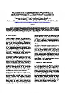
Layer 1 Human actors/ Communication networks

Layer 2 Land and water markets

Agent po pu

96 to 99 90 to 95 84 to 89 78 to 83 72 to 77 66 to 71 60 to 65 54 to 59 48 to 53 42 to 47 36 to 41 30 to 35 24 to 29 18 to 23 12 to 17 6 to 11 0 to 5

lation Seed=5 77

20 15 10 5 0 5 10 15 % of po 20 pulation e (A) Baselin dit (B) A + cre hnologies (C) B + tec

Males

0.15

0.10

0.05

0.00

Layer 5 Ownership

e poverty lin

Layer 4 Farmsteads

Females

0.20

ity Kernel dens

Layer 3 Landuse/ cover

0

5

10

15

20

r] /capita/yea llion joules Poverty [bi

Layer 6 Soil quality

Layer 7 Water flow

Thomas Berger, Pepijn Schreinemachers & Thorsten Arnold Josef G. Knoll Professorship for Land Use Economics in the Tropics and Subtropics, University of Hohenheim

25

2

MP-MAS Software Manual

MATHEMATICAL PROGRAMMING-BASED MULTI-AGENT SYSTEMS TO

SIMULATE SUSTAINABLE RESOURCE USE IN

AGRICULTURE AND FORESTRY

Thomas Berger Pepijn Schreinemachers Thorsten Arnold

Contact: University of Hohenheim (490d) 70593 Stuttgart, Germany Phone +49 711 2459 4117 Fax +49 711 2459 4248 Email [email protected]

A software manual Version 5 June 2007

3


TABLE OF CONTENTS

1

INTRODUCTION .......................................................................................... 4

2

THE INPUT FILES ........................................................................................ 6

3

MATRIX.XLS .............................................................................................. 9

4

POPULATION.XLS ..................................................................................... 19

5

MAPS.XLS............................................................................................... 23

6

NETWORK.XLS ......................................................................................... 24

7

DEMOGRAPHY.XLS .................................................................................... 27

8

PERENNIALS.XLS ...................................................................................... 28

9

LIVESTOCK.XLS ........................................................................................ 29

10

SOILS.XLS .............................................................................................. 29

11

MARKET.XLS ........................................................................................... 30

12

BASICDATA.XLS ....................................................................................... 34

13

SCENARIOMANAGER.XLS ............................................................................ 35

14

RUNNING THE MP-MAS MODEL ................................................................... 37

15

THE X-FILES ........................................................................................... 44

16

SCENARIO OUTPUT FILES ............................................................................ 50

17

GLOSSARY OF TERMS ................................................................................. 53

18

LITERATURE ............................................................................................ 53

1

Introduction

Mathematical programming-based multi-agent systems, MP-MAS for short, is a software tool for simulating sustainable resource use in agriculture and forestry. It can capture both socioeconomic and biophysical dimensions of the farming system. In the MP-MAS, each real world farm household is represented by a single computational agent. Mathematical programming models are used to represent farm household decision-making. The use of mathematical programming to model farming systems builds on a long tradition in agricultural economics (Hazell and Norton 1986). The MP-MAS adds two new features to this tradition. First, whereas the traditional modeling approach relied on the identification of representative farm households, the MP-MAS represents each individual household and landscape unit and hence allows a more complete capture of real world heterogeneity. Second, interaction between households (both spatial and a-spatial) can be implicitly modeled in the MP-MAS. One example is the diffusion of innovations: agents gain access to innovations through communication in their network, after gaining access the agent’s decision to adopt or not adopt is simulated by solving a MP model.

1.1

MP-MAS applications

Balmann (1997) first combined mathematical programming in an agent-based model of land use-/cover change applied to a region in southern Germany. Berger (2001) built forth on Balmann’s model in an empirical application to Chile and used it to simulate water allocation and technology diffusion. Berger and Schreinemachers (2006) extended the model in an empirical application to Uganda to simulate food security. Other empirical applications to Ghana, Thailand, and Vietnam are currently being developed.

1.2

Use of the MP-MAS software

MP-MAS is available as a freeware software that can be downloaded from http://www.uni-hohenheim.de/mas/. This manual is available electronically from the

5


same location. The software is a single executable file that does not need installation. Both a Windows and a UNIX version are available and the program runs on any personal computer. For larger models, the use of Unix OS is recommended as the program runs more stable. The MP-MAS uses optimization software, which needs to be preinstalled. Currently the Optimization Subroutine Library (OSL) is used, which gives a high performance on very large models and can handle many integers (Wilson and Rudin 1992). IBM, the producer of OSL, has stopped the development of its software and transferred the

source

code

to

an

open

source

community

(http://www.coin-

or.org/resources.html). This new solver, called COIN, is currently being implemented to replace the OSL. The number of agents in the downloadable version is limited to 50. MP-MAS is not an open source code software but interested academic software developers can join the group’s effort and contribute to the software’s development. People interested in applying the software to their own research area are also encouraged to get into touch and potential extensions of the software to a particular application can be discussed. The software is constantly being improved: additional features are added with each new application, the input files contain more explanatory information, the error handling of the program is improved, and more powerful solvers (all freeware) are being integrated. Although the model has integrated many new features in recent years, most applications will require additional ones. Interested parties are very welcome to join or link to the research group to put their ideas into additional software code.

1.3

Use of the manual

The purpose of this manual is to make MP-MAS more widely accessible and increase its use by other researchers. The MP-MAS does not have its own graphical user interface (GUI). Instead, Microsoft Excel workbooks are used to organize the data and to setup simulation experiments while the MP-MAS can be run using simple command line functions.


2

6

The input files

MP-MAS works with a set of input files that are read and processed. It is hence different from many software applications in that the input data are not entered through specially designed graphical user interfaces but the user is more or less free to organize the own data. Input files are written in Microsoft Excel workbooks. Most input files contain one data-sheet and one notes-sheet with a brief explanation. The advantage of using Excel workbooks is that most potential users will be familiar with it. It is furthermore convenient as workbooks are easily linked and can contain separate sheets for calculations and documentation of the model. Comments, explanations, and whole calculations can thus be kept together with the final input data which greatly simplifies its use and re-use. The disadvantage is that `small changes can have big consequences’; that is, accidentally entering a value in the wrong place can make the program crash. There are ten input files in the default data set and listed in Table 2. Each input file, except for BasicData.xls, contains data for a specific component of the model. The number of input files can vary between applications as some components are optional. The first file is the mathematical programming matrix (Matrix.xls), which simulates the decision-making of all agents. The following three files contain all information to create agent populations: agents’ resource endowments (Population.xls), their spatial attributes (Maps.xls), and their knowledge of and access to innovations (Network.xls). Then follow four files that model various dynamics over time: demographic changes in agents’ household size and composition (Demography.xls), growth of trees and changes in input requirements (Perennials.xls), the changes in livestock herds (Livestock.xls), and changes in market prices (Market.xls). The tenth file contains data that relate to multiple other input files, hence the name BasicData.xls. Finally, the eleventh file, called ScenarioManager.xls, helps the user to organize the data, convert it to plain text files, and set up various scenarios.

7


Table 1: Input files

Nr.

Input file name

1.

Matrix

Optio

Explanation

Function

The programming matrix (Mixed Integer

Simulates agents’

Linear Program or MILP)

decision-making

-nal no

2.

Population

no

3.

Map

no

Used to generate agent populations All spatial information including the location of agents and plots

4.

Network

no

Define initial agent characteristics

Connects agents by an innovation network and gives details about each innovation

5.

Demography

no

Specifies the life span of agents, fertility, mortality, and available labor hours Define the changes

6.

Market

no

Market prices (exogenous price information)

7.

Perennials

yes

Specifies the time related attributes of

human ageing, tree

perennial crops (yield,

and livestock growth,

over time (e.g.,

price changes)

8.

Livestock

yes

Livestock attributes

9.

Soils

yes

Crop yields and soil dynamics

10.

BasicData

no

Some fixed basic parameter values

11.

ScenarioManager

no

Contains VBA macros that covert Excel workbooks to ASCII format and manages simulation experiments

Before using the MP-MAS, all Excel data-sheets are to be converted to plain text files in ASCII format with the extension “.dat”. This is handled by the Microsoft Excel workbook . This file contains software code (i.e., macros) written

in

Visual

Basic

(VBA)

that

convert

each

file

separately.

For

ScenarioManager.xls to work properly, some conventions about the input files need to be taken care of: 1.

Name of the worksheets. The name of each input file is derived from a prefix specified in ScenarioManager.xls plus the name of the Excel worksheet. For example, if the prefix is set to “A” and the worksheet is named “MILP” then the


8

input file will be called “D_MILP”. The program will not work if worksheet names are changed. 2.

Order of the data-sheets. Each Excel input can contain multiple worksheets. The number of worksheets that is converted to a plain text file is controlled through ScenarioManager.xls in the upper table. If, say, two worksheets are to be converted then the workbook is opened and the first two sheets are taken. Hence the order of the worksheets is important: putting a sheet with calculations or notes first then this one will be converted and the program will not work.

3.

Cells colored red. Good input files need to be well documented with lots of notes and explanations. Yet when converting the input file into plain text format, then all notes have to be omitted. To indicate the program what data should be cleared, the first cell in a row or column is colored red. If a cell in row 1 is red this means that all values in this column will be cleared when converting the workbook to text format; similarly, if a cell in column A is colored red then this means that all values in the respective row will be cleared.

4.

Cell names. Cell names serve two purposes. First, all references between workbooks use cell names. For example, workbook A has a reference to a value in cell $B$2 in workbook B. Imagine now that workbook B is open while workbook A is closed. The reference to cell $B$2 would not change when inserting an additional row at the top of workbook B, though actually the reference should now be $C$2. This problem is averted by using textual cell names instead of references, e.g. give the cell $B$2 the name “GrowthRate” using the Name Box feature of Excel. Second, cell names are used to tell the VBA code about the location of a specific parameter value. For instance, the first value in a block of values, or the end of the sheet.

5.

Text colors. Some values are internally calculated in the data-sheets while others are referenced to other workbooks. Different text colors are used to identify these. The following five colors are used:

9


Table 2: Text color uses Color of text

Meaning

blue

Numbers that are linked to other cells in the same workbook

red

Numbers that are linked to another workbook

pink

Numbers that are updated when running ScenarioManager.xls

black

Numbers that can be changed

Table 3: Cell colors uses Background color of cells

ColorIndex (VBA) 3

red

43

green light yellow

3

-

Meaning These columns and rows will be deleted when using the MAS and when using the stand alone Solver Normal cells (Matrix.xls only) These rows will be deleted when using the stand alone solver but not when using the MAS (Matrix.xls only) The first and last activities of the matrix, which should all have values zero.

Matrix.xls

Matrix.xls contains a mathematical programming model, which is a mixed integer linear programming model (MILP). This model optimizes the expected net household income. This includes expected income from farm, non-farm, and off-farm labor and includes current as well as future expected income streams. To perform the optimization for every agent, first a general programming matrix is defined that can capture the activities and constraints of every agent. The MP-MAS then changes the resource endowments (right-hand-side values) and switches on and off activities and constraints, to tailor each mathematical program to a specific agent. Although all MPs are agent-specific, there is therefore no need to define each MP individually; the software handles this using data from all other files. Matrix.xls is a special file because it is here that data from all other files come together. Prices are derived from Market.xls, initial resource endowments come from Population.xls, input-output data for livestock and perennial crops come from

10


Livestock.xls and Perennials.xls, while access to innovations comes from Network.xls. All these files are linked to Matrix.xls for each data input file contains information on where in the programming matrix these data have to be inserted. The exact location in the matrix is communicated using activity and constraint indices. Furthermore, the activities and constraints need to be ordered in a specific way. The matrix-file specifies 16 categories of data to be entered, of which one (category 4) is the programming matrix. The categories are listed and described in Table 4.

Table 4: Data categories in the Matrix-file Nr.

Name

Brief description

1

Parameters and coefficients

2

Activity type

3 4

Objective function coefficients Programming matrix

Tells the MP-MAS if and how many “special” activities are included in the matrix. E.g. irrigation, credit, etc. Selling and buying activities are indicated as “0”, while all other activities as “-1”. Buying and selling prices.

5

Parameter values

6

Binary for disinvestments

7

Fixing of columns in "consumption mode"

8

Fine tuning parameters

9

TSPC input for cropping activities in NRUs

10

13

Column indices for stover use for livestock feeding Column index for manure accounting Type and range of constraints Marked integers

14

Lower bounds on columns

The minimum value to which an activity can be selected

15

Upper bounds on columns

The maximum value to which an activity can be selected

16

Integers sets / SOS

Special integer treatment to speed up solution in the case that the MILP includes many integers.

11 12

The specification of activities and constraints. No missing values are allowed, zeros need to be entered explicitly. Fixed/independent constraints can be included, for instance if a right-hand-side value should always take a value 10. In addition, fixed costs can be included here and specified as a function of farm size (in ha). These coefficients specifically relate to the three-stepconsumption model (see market file) and should be left blank if this model is not used. These coefficients specifically relate to a three-stage optimization procedure of sequential investment, production, and consumption decisions (see text). Can be used to alter crop yield expectations when taking production decisions to capture risk. These coefficients relate to the use of the Tropical Soil Fertility Calculator to simulate soil dynamics and crop yields, and should be left blank if this model is not implemented. Idem. 9 Idem. 9 Relates to the sign of the constraints (see text) Indicates which activities are integers

11


3.1

Structure of the programming matrix

The programming matrix needs to be structured in a pre-determined order for activities and constraints. Figure 1 shows this structure schematically. More details follow. Figure 1. Schematic overview of activities and constraints in Matrix.xls Activities Selling of crops and Empty livestock

Buying inputs

Credits & Acess to deposits innovations

Livestock

Growing crops

Selling future products Empty

Empty Cash

Constraints

Labor use Land Livestock Perennials Innovations Credit Crop yield balances Empty

Table 5: Order of activities in the programming matrix Activities

Explanation

A.

First activity

empty, filled with zeros

B.

Selling and buying activities

All these activities have objective function c1oefficients

Short-term deposits

(prices) and have to appear in exactly the same order as

Hiring in labor Hiring out labor C.

All other activities

D.

Future revenues from investments

in the first block of entries in the market file. For each period, the price vector is copied and pasted into the MATRIX file. The order does not matter Activities with objective function coefficients for selling of future products (e.g. meat, coffee, etc.)

E.

Last activity


Table 5 shows the correct order of the activities. The first and the last activity is not used and should be filled with zero values. These activities are important since they have cell names that should not be changed; leaving them blank ensures that no activity that is inserted replaces the first or the last activity with the cell names. All selling and buying activities follow next. It is important that these activities have the

12


same order as in the market file where their prices are listed for each simulation period. Hiring in labor should come before hiring out labor. After all activities that have prices, come all other activities. These can be ordered using any logic. Lastly come activities that can add to the objective function.

Table 6: Order of constraints in the programming matrix

A.

Activities

Explanation

First constraint

empty, filled with zeros but has an entry of “1” for investments in perennial crops

B.

Liquid means

Transfers the liquid means from the right-hand-side into the activities

C.

Labor

Labor endowments (can be age and sex-specific)

Land

Land endowments (can sub-divided into soil classes)

Irrigation

Amounts of available irrigation

Livestock

Livestock endowments in heads

Perennial crops

Hectares of existing plantations

Access to innovations

Controlled by the network-file, a positive value is entered here if an agent has access to an innovation and zero otherwise

D.

Capital use in period 0

Required capital in period 0 of the investment, i.e., the initial start-up cost

Capital use in average year

Average amount of capital required

Short-term credit

The amount of short-term credit required for an activity

E.

All other constraints

The order doesn’t matter here

E.

Last constraint


Table 6 shows the correct order of the constraints in the programming matrix. Like in the activities, the first and the last constraints are best left blank, i.e., filled with zeros, as these have cell names that should not be changed. The first constraint controls whether the model is an investment or a production problem. If it is an investment problem, then investment goods such as tree plantations and livestock can be purchased; if it is a production problem then this option is not available. This constraint switches the investment possibilities for perennial crops on by inserting a value in the right-hand-side. This is followed by a flexible number of constraints that determine the resource endowments of each agent. This includes liquid means (the

13


third constraint), which is the amount of accumulated savings by the agent, which is available for investment, variable inputs, or market consumption. This furthermore includes, available amount of labor, land, livestock, and areas of plantations, each of which can be subdivided into many categories (e.g., labor into different age groups, land into soil fertility classes).

3.2

Splitting the programming matrix

Microsoft Excel is limited to 256 columns but it can handle up to 65,536 rows. When specifying a programming matrix, the number activities are usually much greater than the number of constraints and also often greater than 256. There are two ways to overcome this limitation in Excel by splitting the matrix into smaller parts. The MP-MAS can handle both. First, the programming matrix can be split in vertical blocks, which are then ordered vertically as shown in Figure 2. Second, the matrix can be split horizontally and each block can then be transposed as shown in Figure 3. In both methods, the division in blocks adds the inconvenience of either duplicating activities or constraints. For instance, when splitting and transposing the matrix, then when adding an activity, then this activity has to be added to each block separately. Hence, the number of additional blocks is best kept to a minimum.

Figure 2: Splitting a programming matrix ACTIVITIES

ACTIVITIES

ACTIVITIES

CONSTRAINTS

CONSTRAINTS

CONSTRAINTS

CONSTRAINTS

ACTIVITIES

14


Figure 3: Splitting and transposing a programming matrix CONSTRAINTS ACTIVITIES

ACTIVITIES

CONSTRAINTS

ACTIVITIES

CONSTRAINTS

ACTIVITIES

CONSTRAINTS

Since there are typically fewer constraints than activities, the split and transposed matrix requires fewer blocks. It has the additional advantage that the equations (i.e., the constraints) are kept together in the blocks, which makes it easier to read. The disadvantage for experienced LP-modelers is that thinking in terms of constraintcolumns and activity-rows requires a change in thinking. When splitting the matrix, then the number of blocks has to be entered in data category 1.10 of the data-sheet. In addition, it has to be specified whether the matrix is transposed or not and the first constraint and activity index of each matrix block (on indices see below). The default data set contains both a normal and a transposed matrix. The VBA reads the matrix in the first sheet, so if the transposed matrix is to be used, then the order of the sheet must be changed.

3.3

Additional information for the activities and constraints

3.3.1 Use of activity and constraint indices Activities and constraints are identified using an activity and constraint index that starts with zero (index = 0,1,2, …n). The index of the first activity has the cell name iact_0 while the index of the first constraint has the cell name icon_0. When inserting or deleting activities and constraints, it is important that the indices are updated. If

15


not, then the VBA will give a warning message when converting the workbook to ASCII format. Because the first and the last constraint as well as the first and the last activity have various cell names that are referenced, they are best left unused and filled with zero values only. In the data-sheet, these are marked using a shade of yellow.

3.3.2 Information about the activities Figure 4 shows the upper left corner of the first block of the transposed programming matrix. Figure 4: The programming matrix

Activities are ordered in rows, while constraints are ordered in columns. For each activity, 10 types of information need to be specified (ordered a-j). The first five of these, are only to assist the model builder as these are not read by the MP-MAS: a) The activity index as explained above, staring with number 0. b) The name of the activity, which should ideally be short and clear.


16

c) The unit of the activity (e.g., hectare, kilogram, $, etc.). d) The solution vector, or also called the decision variable, which is used to evaluate the optimal outcome. e) The objective function, which is only required when using the stand-alonesolver. When using the MP-MAS, than it should contain as prices are derived from the market file. The product of the objective function and solution vector is what is optimized. The following five variables are required by the MP-MAS: f) The type of activity, which is “0” for selling and buying activities; “1”for Growing an irrigated annual crop; “2” for growing an irrigated permanent crop; “3” for divisible investment goods with irrigation; “4” for indivisible investment goods without irrigation; and “-1” for all other activities. Based on the information, the MP-MAS, among other things, calculates the income balance. g) Market integers, which is 1 if the activity can only obtain integer values, and 0 otherwise. h) Fixing in consumption mode, this only applies to the use of a three-stage optimization procedure of sequential investment, production, and consumption decisions. When set to 1, then the selected activities in production mode cannot be changed in the consumption mode. This captures the timely sequence and irreversibility of investment and production decisions. When using the one or two-stage optimization, than all values should be set to 0. i) Lower bounds on the activities, which is the minimum value the decision can take. j) Upper bounds on the activities, which is the maximum value of the decision. The variables f-j are specified left of the programming matrix as shown in. This is only to minimize errors. The MP-MAS requires these data to be ordered sequentially in the same order as listed in Table 4. Manually entering these data in this order is cumbersome, especially when the programming matrix is large. This procedure is therefore automated using the VBA. To do this, the VBA needs to know the location where the information has to be copied from and where it has to be pasted to. This is provided using cell names as listed in Table 7.

17


Table 7: Cell names of activity information Matrix-file cell names Data category

Copied from

Pasted to

e.

Objective function coefficients

ObjFunctionCopy0

ObjFunctionPaste

f.

Activity type

ActTypeCopy0

ActTypePaste

g.

Marked integers

IntegerCopy0

IntegerPaste

h.

Fixing in consumption mode

FixConsCopy0

FixConsPaste

i.

Lower bound

ActLBoundCopy0

ActLBoundPaste

j.

Upper bound

ActUBoundCopy0

ActUBoundPaste

Cell names for the first block of values to be copied end with “0”. If the programming matrix contains multiple blocks of values, as suggested in Figure 2 and Figure 3, then these cell names should be adjusted to end with 1, 2, etc.

3.3.3 Information about the constraints Figure 4 also shows the constraints ordered in columns. For each constraint, there are seven types of information added to the matrix: 1) Type of constraint, which is directly related to the sign of the constraint equation: a value of 1: “smaller or equal than”; 2 “greater or equal than”; and 3 “is equal to”. 2) Range of the constraint, also this directly relates to the sign of the constraint equation: a value of 1: “-1E+31”; a value of 2: “-1E+31”, and a value of 3: “0”. 3) The left-hand-side, which is only used for evaluating the programming matrix and does not have to be filled in. 4) The sign, smaller or equal than (“≤”), greater or equal than (“≥”), or is equal to (“ =”). Note the use of one space before the is-equal sign, because Excel would otherwise treat this sign as a formula. 5) The right-hand-side, which is only used in the stand-alone-solver version. Right-hand-side values are agent-specific and are constructed from an agent’s resource endowments (land, labor, knowledge, etc.). 6) The unit of the constraint, e.g. kilogram, hectare, etc. This is not obligatory and is not read by the MP-MAS

18


7) The constraint index, which is neither directly used by the MP-MAS, but is however very important, as other cells are referenced through this index to specific locations in the matrix. Like in the case of the activities, the MP-MAS requires these data in a specific order as listed in Table 4. This ordering is handled by the VBA and only needs a correct specification of cell names as shown in Table 8. If using the split and transposed matrix, than the constraint-related data needs to be read from separate blocks. The cell names need therefore to be given for each block separately. The cell names in block 1 get the suffix 1, in block 2 the suffix 2, etc.

Table 8: Cell names of constraint information matrix-file cell names Data category

Copied from

Pasted to

1)

Type of the constraint

ConTypeCopy0

ConTypePaste

2)

Range of the constraint

ConRangeCopy0

ConRangePaste

3)

Right-hand-side

RHSCopy0

RHSPaste

Developing the programming matrix is the most time consuming part of building the MP-MAS. Large matrices are best build step-by-step, adding one feature at a time and then trying it before adding another feature. This involves frequent solving of the programming matrix. To facilitate this process, the MP-MAS has a stand alone solver to check the programming matrix separately from all the other input files.

This

stand-alone solver can be run from the file and is explained in Section 15.4.

19


4

Population.xls

The population file contains two types of information: (1) the demographic composition of the population (age and gender); and (2) the asset composition of the population (livestock, machinery, area of tree plantations, and liquidity). The methodology is based on Monte Carlo techniques, which is shortly described in the following. 4.1

Use of Monte Carlo techniques

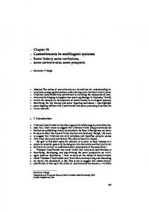
The methodology to randomly generate agent populations from a sample of farm households is based on Monte

Figure 5: Empirical cumulative distribution of goats over all households in the sample

Carlo techniques. The objective is to generate a multitude of potential agent populations,

with

all

agents

being

different both within a single population and between different populations. One of the challenges in generating an empirically based agent population is to represent

each

real-world

farm

household with a unique agent. Yet, data are often available only for a sample of the farm household population. The challenge hence became how to extrapolate the sample population to generate the remaining non-sample agents. The most obvious route would be to multiply the sample farm households with their probability weights. Average values in this agent population would exactly equal those of the sample survey. Yet, this copy-and-paste procedure is unsatisfactory for the several reasons. First, it reduces the variability in the population. For instance, a sampling fraction of 20 percent would imply about five identical agents, or clones, in the agent populations. This might affect the simulated system dynamics, as these agents are likely to behave analogously. It becomes difficult then to interpret, for instance, a structural break in simulation outcomes; e.g., is the structural break endogenous, caused by agents breaking with their path dependency, or is the break simply a computational artifact resulting from the fact that many agents are the


20

same? This setback becomes more serious for smaller sampling fractions, because a higher share of the agents is then identical. Second, the random sample might not well represent the population. The sample size is small and the sampling error is unknown but can be large. When using the copy-and-paste procedure, only a single agent population can be created, while for sensitivity analyses a multitude of potential agent populations would be desired. For these reasons, the procedure for generating agent populations is automated using random seed numbers to generate a whole collection of possible agent populations. Monte Carlo studies are generally used to test the properties of estimates based on small samples. It is thus well suited for the present purpose as data about a relatively small sample of farm households is available but the interest goes to the properties of an entire population. The first stage in a Monte Carlo study is modeling the data generating process, and the second stage is the creation of artificial sets of data. The methodology is based on the use of empirical cumulative distribution functions (ECDF). Figure 5 illustrates such a function for the distribution of goats. The figure shows that 35 percent of the farm households in the sample have no goats, the following 8 percent has one goat, etc. This function can be used to randomly generate the endowment of goats, and all other resources, in an agent population. For this, a random integer between 0 and 100 is drawn for each agent and the number of goats is then read from the y-axis. Repeating this procedure many times recreates the depicted empirical distribution function. Each resource can be allocated using this procedure. Yet, each resource would than be allocated independently, excluding the event of possible correlations between different resources. However, actual resource endowments typically correlate, for example, larger households have more livestock, and more land. To include these correlations in the agent populations, the sample is divided into a number of clusters based on statistical analysis (e.g., using cluster analysis). In this example, nine clusters are formed based on the variable household size, as this variable correlated most strongly with all other variables. Cumulative distribution functions are then calculated for each cluster of sample observations. This is illustrated in Figure 6 for the random allocation of goats to the agents.


21

Figure 6: Cumulative distribution of goats over households per cluster

4.2

Implementation in the MP-MAS

The ECDFs are included in the file . This file includes a separate data-sheet for each cluster (hence nine files in the above example). In each datasheet two blocks of information appear. The first block relates to the agents’ household age and sex composition, while the second block relates to all other assets. As most resources only come in discrete units (e.g., number of agent household members, heads of livestock), a piecewise linear segmentation is used to implement the distribution functions. The default is five linear pieces but more can be specified in the need arises. Table 9 shows an example for the first block of information related to the household composition. The abbreviation “UB” stands for upper bound, while the abbreviation “UV” stands for upper value. The first line in this table is interpreted as follows. An object names “m04” is allocated to the agents in this cluster. This object has an ID of 50, and its sex is 1 (male). The lower age limit of this object is 0 and the upper age is 4. Every agent in this cluster has a probability of 40% (UB1) of having 0 members (UV0) in this category, a probability of 30% (70-40) of having 1 member, a

22


probability of 10% (80-70) of having 2 members, a probability of 10% of having 3 members, and finally, a probability of 10% (100-90) of having 4 members in this category. Table 9: Demographic composition Object

ID Sex Lower Upper

UB1

UV1

UB2

UV2

UB3

UV3

UB4

UV4

UB5

UV5

m04

50

1

0

4

40

0

70

1

80

2

90

3

100

4

m59

50

1

5

9

50

1

90

2

100

3

0

0

0

0

m1014

50

1

10

14

20

0

50

1

90

2

100

4

0

0

m1519

50

1

15

19

30

0

50

1

80

2

90

4

100

5

m2024

50

1

20

24

40

0

80

1

100

2

0

0

0

0

m2529

50

1

25

29

70

0

80

1

100

2

0

0

0

0

m3034

50

1

30

34

80

0

100

1

0

0

0

0

0

0

m3539

50

1

35

39

90

0

100

1

0

0

0

0

0

0

… Note: UB and UV stand for "upper bound" and "upper value" respectively, of which the UB is expressed cumulatively as a percentage of total agents.

The second block of information is the similar, except that these objects have no sex and no lower and upper age limit, but can optionally have a land requirement (Table 10). The objects include livestock (e.g., cows and goats), a farm structures (e.g., a henhouse), or hectares of coffee plantation: 1. a female head of the household 2. innovation segment: early adopters to laggards 3. form of expectations: rational, .. 4. liquidity: liquid means available for investments 5. leverage:… The specification of these five assets is not optional. If no data on these are available, then all values are to be set to zero.

23


Table 10: Asset composition Object

ID

Type

LR

UB1

UV1

UB2

UV2

UB3

UV3

UB4

UV4

UB5

UV5

Female head

44

-1

0

100

1

0

0

0

0

0

0

0

0

Innovat.

45

-2

0

10

1

40

2

60

3

80

4

100

5

Expect.

46

-3

0

29

0

100

2

0

0

0

0

0

0

Liquidity

47

-4

0

100

500

0

0

0

0

0

0

0

0

Leverage

48

-5

0

89

0

95

0

100

0

0

0

0

0

Cow

2

8

.91

50

0

70

2

80

4

90

7

100

23

Goat

3

8

.13

40

0

60

1

80

3

90

4

100

8

Cow in shed

4

8

0

100

0

0

0

0

0

0

0

0

0

14

1

1

30

0

40

0

60

0

80

0

100

4

Coffee 1 …

Note: LR stands for land requirement; UB and UV stand for "upper bound" and "upper value" respectively, of which the UB is expressed cumulatively as a percentage of total agents.

5

Maps.xls

MAS models of land-use/cover change (MAS/LUCC) couple a cellular component that represents a landscape with an agent-based component that represents human decision-making (Parker et al 2003). The landscape component is defined in the map-file. It contains six spatial layers of information as summarized in Figure 10. The information is numerically encoded and organized in a raster format. Grid cells with no information get a value “-1”. Each cell represents a certain amount of land, e.g., 1 hectare. The map-files can be produced in two ways: in a Microsoft Excel workbook, if the number of columns is less than 256 and which is then converted to plain text format using ScenarioManager.xls, or in ArcView GIS using the exporting routine to save it in ASCII format. All maps have to be in a grid cell format. Polygons must be converted to grid cells. Yet, by defining the grid sufficiently small, the grid format can approximate any polygon.

24


Table 11: Spatial layers in Map.xls Nr.

Layer

1.

The location of agents’ farmsteads

2.

Each agents’ membership of a population

3.

Each agents’ membership to a population cluster

4.

Each agents’ membership to an innovation segment

5.

The location of agents’ plots

6.

The soil type of each plot

Figure 7 shows an abstract of a very simple map-file in Excel for the location of farmsteads. This simple landscape shows two farmsteads (coded with IDs 0 and 1). All locations without a farmstead should be denoted with “-1”. Note that when using the downloadable version of MP-MAS, the maximum number of farmsteads that can be included is 50. Figure 7: Example spatial layer for the location of farmsteads 2

6

LOCATION OF FARMSTEADS (ID)

-1

-1

-1

-1

-1

0

-1

-1

-1

-1

1

-1

-1

-1

-1

-1

Network.xls

Population.xls randomly assigned each agent to a network segment. The file Network.xls can be used to control the access of agents to innovations. If all agents have access to a particular technology (e.g. a traditional crop variety), then this technology does not have to be included in the Network.xls, yet if the technology is relatively new (i.e., an innovation) and is only partially diffused in the sample population, then the network file can be used to represent this partial diffusion. The diffusion of innovations is based on a network threshold model (Valente 1994). This type of model is based on the idea that information diffuses gradually through

25


interpersonal networks and that once enough information has reached a particular agent, it will then consider adoption. How much information is ‘enough’ is agentspecific and determined by the threshold level. In line with Valente (1994), five network thresholds are specified as shown in Table 12. Agents that belong to the group of early adopters (nr.2) will only consider adoption after the group of innovators has adopted, that is when the adoption rate has reached 2.5 percent. Table 12: Network threshold values

1

Threshold

Characterization

< 2.5%

Innovators

2

2.5 – 16%

Early adopters

3

16 – 50 %

Early majority

4

50 – 84 %

Late majority

5

84 – 100 %

Laggards

The actual adoption decision is both a function of these individual network thresholds and the expectations of agents. Agents will only adopt if (a) they have reached their network threshold; (b) they expect the innovation to bring a positive net contribution to meeting their objectives (it brings an agent utility). This two-stage adoption procedure yields a realistic way of simulating the diffusion of innovations. Agents’ membership to network thresholds was assigned Population.xls. The diffusion model is sensitive to the proportion of agents in each network. The allocation of many agents to the first segment will speed up the diffusion of innovations, while the diffusion will be stagnant if less than 2.5 percent of all agents are allocated to the first segment. Ideally, the distribution of agents follows the threshold values -- that is 2.5% is defined as innovators, 13.5% as early adopter, 34% as early majority, etc. This can, however, not be guaranteed as the assignment to network groups is partially random. To overcome this, a calibrating factor called ‘overlap’ is included. The overlap factor is multiplied by all network thresholds and can attain values between 0 and 1. If set to 1, then the network thresholds are unadjusted, while if set to 0, then all thresholds become 0 and all agents can hence immediately adopt. The model needs to be tested for an appropriate value of the overlap factor (most usually it will have to be set to values between 0.5 and 0.8).

26


Table 13: Innovations Nr.

Parameter

1

Object ID

Explanation This should match with the object ID in all other files (e.g. , , and .

2

Type

The type of object. There are two basic types: Objects with a negative type refer to agent characteristics, while objects with a positive type refer to asset characteristics (incl. innovations).

3

Divisibility

Set to 1 for all divisible innovations. E.g., a cow is indivisible (set to 0) while a hectare of coffee is divisible (set to 1)

4

Acquisition costs

The purchasing price of an innovation in the first year. For livestock, make sure this is consistent with . Note that this cost refers only to “proper investments”, i.e. productive activities with a gestation between first input use and full output of more than 1 year. If shorter than 1 year, then the price must be included in file .

5

Lifetime

The maximum age of an object. For example, a coffee plantation lasts 12 years, and cows are culled before they turn 10 years old.

6

Suitability

The soil types an innovation can be used on, if not restricted to any soil type then set the suitability to 0.

7

8

Minimum

Optionally a minimum amount can be specified. E.g, when investing into a new

investment

coffee plantation, the investment should be more than 0.2 ha.

Column

The activity index in the programming matrix. In case of investment objects, the MATRIX includes two separate activities: one for production and one for investment. This index must refer to the production activity.

9

Row

The constraint index in the programming matrix.

10

Permanent crop

The row coordinate in the programming matrix where the yields appear (-1 if not

yield

a permanent crop)

Coefficient

The pieces per unit of the investment good (e.g., days/laborer)

11

The solution in the investment mode is taken and enters the production mode after multiplication with this factor. The factor is therefore used to convert the units in the solution vector of the investment mode to units of the RHS in the production mode. 12

Level of

Specifies for what segment the innovation is accessible, if accessible for all set to

innovation

0.

13

Availability

The year at which the innovation is introduced into the population

14

Accessibility

The year at which the innovation can be acquired for the particular innovation segment.

15

Share own capital

The share of the acquisition cost that needs to be paid from own liquid means.

16

Interest rate on

For what is not paid from own means an additional interest cost is incurred.

borrowed capital

27


Network.xls lists all innovations and specifies various types of information for each of these as is briefly explained in Table 13. The network-file uses three types of interest rates. (1) The long-term interest rate is the interest over borrowed capital with a gestation of longer than one year. (2) The short-term interest rate is the rate for borrowing capital from, say a bank, for a period of one year. (3) The interest rate on equity is the rate you receive when depositing money at a bank (say, at your current account). This is the opportunity costs of capital. In absence of any banks or informal savings, this rate can be set very low.

7

Demography.xls

The age of each household member naturally changes over time. Aging impacts on the household labor supply and is therefore an important dynamic in the model. Demography.xls specifies age-specific variables that optionally include, apart from labor supply, mortality, fertility, and nutritional requirements. Table 14 shows an abstract of this file, for the labor category of unskilled male labor for the first 4 years. Table 14: Abstract of the demography file B. Unskilled male members Career ID

64

Number of different ages (lifespan)

100 Age 0

Age 1

Age 2

Age 3

1

1

1

1

Labor hours / year

0.0000

0.0000

0.0000

0.0000

Mortality (probability of dying)

0.0764

0.0257

0.0123

0.0074

Fertility (probability of giving birth)

0.0000

0.0000

0.0000

0.0000

Sex-age group

Energy needs (billion joules/year)

1.0684

1.5055

1.7312

1.8747

Protein needs (kg/year)

5.1100

8.0300

8.0300

9.4900

Labor supply can be estimated from farm household survey data. If the programming matrix uses an agricultural production function that relates output to labor use, then it is important that the labor supply is estimated from the same data source. Data on time

allocation

are typically

inaccurate

and

variable

between

surveys.

The


28

importance here is not so much to get an accurate estimate but an estimate that is consistent with the production function used. Mortality and fertility are specified in terms of the probabilities of dying and giving birth. Mortality and fertility can be obtained from official statistical sources or demographic studies. Make sure that the probability of dying at the maximum age is set to unity otherwise the program might crash. Food nutrition, such as calories and protein, can be included to quantify food security. This is only useful in case a detailed food consumption model is included that estimates food consumption into detail. This consumption model, simulating the nutrient supply, would have to be specified in Market.xls; while Demography.xls estimates the nutritional demand and the balance of the two would be an indicator of food security. Food nutrition is location specific and moreover depends on the intensity of physical activity performed. One possible source of country-specific default values is James & Schofield (1990).

8

Perennials.xls

Whereas the population file specifies the course of human life, the permanent crop file specifies that of trees. It contains the following information for each year in the life span of a permanent crop: 1.

yield

2.

pre-harvest costs (e.g., spraying)

3.

harvest cost

4.

total labor requirement

5.

total machinery requirement

6.

peak labor requirements

Furthermore, it specifies the acquisition cost and life span, both of which should be the same as specified in the network file. Because alternative levels of input use are possible for a crop, a separate permanent crop activity is specified for each input level. For instance, in the Uganda case, coffee can be grown on five different soil types, with 3 alternative levels of labor use, and with or without fertilizer; this translates into 30 different coffee activities. Switching


29

between input levels and between soil types is thereby prevented and to switch input levels the agent is required to fulfill the acquisition cost and start anew in year 0.

9

Livestock.xls

The livestock file is similar to the permanent crop file in that different parameter values can be specified for each year. The livestock file is, however, different from the permanent crop file in that more than one output can be specified and the matrix coefficients of these outputs are directly entered in this file, rather than the network file. The first two outputs of each livestock type are gain in live weight, which is specified cumulatively, and numbers of female offspring. Female offspring is treated differently as this has a course of life of its own starting with year zero. Male offspring remains in the file as its sole purpose is meat production. Livestock.xls is furthermore different from the permanent crop file in that it allows labor to be specified per period, while in the permanent crop file only average labor is specified which is distributed over all periods according to fixed coefficients in the programming matrix.

10 Soils.xls Soils.xls contains parameter values for a biophysical model to simulate soil fertility changes and the resulting crop yields as based on the Tropical Soil Fertility Calculator (TSPC). This integrated model was developed for an MP-MAS application to Uganda. For more details about this component the reader is referred to Schreinemachers et al. (2007) and Schreinemachers (2006). The TSPC does not have to be included in the model but can be switched off in ScenarioManager.xls. If switched off then the file soils.xls does not have to be included in the input data.


30

11 Market.xls Market.xls contains two types of information. First, it specifies market prices for all products and second, it specifies which type of consumption model is implemented. Each is described in the following. 11.1

Market prices

Market prices define the prices for all tradable goods and is equivalent to the objective function of the MP model. Market prices include: (1) selling prices of agricultural products; (2) buying prices of food products; (3) buying prices of seed, chicks and fertilizer; and (4) prices of leasing in a tractor, and hiring in or out labor. The MP-MAS software copies these values and pastes them into the MP matrix. The order of these goods must therefore be the same as in the file . All market prices are exogenous in the model and need to be defined for each period in the market-file. The effect of price changes can be simulated by adjusting the prices in this file; this file can therefore be used to test various price-related scenarios. Market prices include the price of hiring labor in and hiring labor out. Make sure that the price of hiring in is greater than the price of hiring out otherwise the MP model might become unconstrained. A higher price for hiring in is justified by transaction and monitoring costs. A special type of prices are ‘future prices’, these are expected selling prices related to investment activities such as livestock or trees. These, for instance, include milk and meat. These products cannot be sold in the same year of investment and hence do not add to the current revenues but only to the future income. Whereas the current prices always enter the matrix in a pre-determined order as the first activities, the user can determine where the future prices enter the matrix by specifying an activity index for each entry. Hence, the order in which they appear in the matrix file does not matter. Activity indices are ideally linked to the matrix-file so that they are automatically updated when adding activities or constraints to the matrix.


11.2

31

The consumption model

Two types of consumption models can currently be specified: one very basic and one very complicated model. More intermediate consumption models will be included in the future. The choice of consumption model should be included in BasicData.xls. If using the extended consumption model then Matrix.xls needs to include the consumption model in the matrix.

11.2.1 The basic consumption model When using the basic consumption model, then consumption is handled by simple heuristics outside the MP model and after the income level has been determined. Buying activities for food products do therefore not have to be specified in the market file. The basic consumption model simply specifies how much of the income will be consumed. The remainder will be added to the agent’s cash endowment and is available for investment in the next period. The basic model requires specification of three parameters: (1) Extra consumption [proportion]: This is the proportion of each additional monetary unit that is consumed and ranges between zero and one. If set to zero then no income is consumed and all is saved; if set to one then all income is consumed and nothing is saved. (2) Minimum consumption per head/year [monetary value]: This value specifies the minimum amount of income that is consumed by each member of an agent’s household. It must be set to a positive value. (3) Foregone consumption [monetary value]: In case that income is too low to meet the consumption specified by (1) and (2) then this value determines the proportion by which the consumption level is to be reduced. If set to zero then the minimum consumption level is reduced to zero. If set to one then the consumption is not adjusted downward.

11.2.2 The extended consumption model If using the extended consumption model then the program uses a three-stage solving procedure of investment, production, and consumption (the last stage is not needed if using the basic consumption model). The assumption is that production

32


and consumption decisions are inseparable because of market imperfections as is typically the case in rural areas of low-income countries (Sadoulet and de Janvry, 1995). Different from the basic consumption model, that simply allocates part of the revenues to consumption and the rest to savings, the extended model implements the consumption decision within the MP model so that production and consumption decisions are simulated simultaneously. Because the parameters of the extended consumption model are household-specific its implementation requires much additional input in both the market- and the matrix-file. The implemented consumption model itself has a three-step procedure of savings, food/non-food expenditures, and expenditures on specific categories of food products. The model is described in Schreinemachers (2006) and Schreinemachers and Berger (2006b). Including this model requires the estimation of econometric models at each step. The advantage of this model is that it allows a detailed simulation of food security dynamics. If food security is not much of an issue and market imperfections are few then the basic consumption model is preferred.

11.2.3 Savings In the first step of the system, agents decide how much of their income to expend and how much to save. Let the variable SAV be the savings and INC the disposable income, H the household size measured in an equivalence scale (joules), D the matrix of district dummies, and α0 a constant term. The amount of savings is specified as a quadratic function of disposable income: n −1

SAV = α 0 + α1 INC+ α 2 INC2 + α 3 H + ∑ α 4,i D

with α 2 > 0

(1)

i =1

in which the alfas are the parameters to be estimated. Micro-economic theory suggests that the share of savings increases with income, which is the case if α2 is positive.

11.2.4 Food/non-food expenditures Total expenditure (TEX) is the income available to spend, which is derived from the income identity:

INC = SAV + TEX

(2)

33


In the second step, agents decide how much of this total expenditure to allocate to food (FEX) and non-food items (NEX). A modified version of the Working-Leser model quantifies this relationship (Hazell and Roell 1983): 40

v = β 0 + β1ln TEX + β 2 H + ∑ β 3 D

(3)

n =1

in which v is the expenditure share on food and the betas are parameters to be estimated. It follows that the value of food expenditures (FEX) equals TEX*v/100 while NEX can be derived from the parameter estimates using the properties of symmetry and adding up.

11.2.5 Expenditures of food categories. In the final step agents decide to spend their food budget on broad categories of food products. The use of categories instead of individual items gives agents more scope for substitution. The third step is quantified using a linear approximation of the Almost Ideal Demand System (LA/AIDS) (Deaton and Muellbauer 1980): 40

w k = δ 0,k + ∑ δ1,k,l ln p l + δ 2,k ln(M/P * ) + δ 3, k H + ∑ δ 4,k D k

(4)

n =1

where the subscripts k and l denote individual food categories of a total of n categories (k,l=1,2,..,n) and the gammas denote parameters to be estimated. The variable wk is the share of category k in the total food budget; M is per capita food expenditures measured in an equivalence scale for household size. P* is an index of prices, which in the original (non-linear) version has a translog functional form but in its linear version can be replaced by the logarithm of the Stone geometric price index (Deaton and Muellbauer 1980):

ln P* = ∑ w k ln p k k

(5)

34


12 BasicData.xls Parameters that do not immediately relate to a single input file but are required by several separate model components are included in BasicData.xls. About 48 parameters are included in this file. For instance, the choice of consumption model is included in BasicData.xls because this impacts both on the matrix-file and on the market-file. The file is organized in eight categories of parameters as shown in Table 15. Most parameters in this file are self-explanatory.

Table 15: Parameters in BasicData.xls Category

Explanation

1

General parameters

Integers counting the frequency of same events, like the number of

2

Innovation parameters

catchments, villages, networks, etc. Various parameters that allow the user to fine-tune the innovation diffusion process, such as the ‘overlap’ parameter described in Section 6. 3

Rental markets

4

Policy parameters

For making land markets endogenous in the model For the simulation of policy options such as subsidies for permanent crops

5

Switches for various sub-

Defines which consumption is implemented and whether there is a crop

models

growth model, livestock or perennial crop model. If not then no respective file is read by the program.

6

Soil information

Defines the size of a single grid cell in hectares and defines which number of different soil types and classes. Soil classes refer to land suitability.

7

Debugging of the

The most important dynamics can be switched off using these options:

programming matrix

(a) aging of agent household members and assets; (b) and updating of soil fertility (only if a soil model is defined). In addition matrices can be saved by entering a matrix number.

8

Fine-tuning of the solver

This tells the solver how long it can maximally take to solve a single MP model or how many iterations is can go through.


35

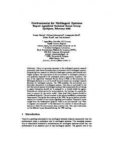
13 ScenarioManager.xls Figure 8 shows the interface of the Scenario Manager. This file can be used to convert all Excel files into plain text format. Map files get the extension “.gis” while all other input files get the extension “.dat” To run macros, the security setting in Microsoft Excel (Tools>>Macros>>Security) should be set to medium or low and macros must be accepted when opening the file. ScenarioManager.xls works with an Excel AddIn called “Mpmas”, which needs to be installed as follows. In Microsoft Excel, go to the menu item “Tools/ Add-ins…”. Click the browse button and find the location of Mpmas.xla. Select this file so that Mpmas appears in the list of Add-ins and make sure the checkbox is selected. The Mpmas add-in is now installed and any time you open Excel, a MP-MAS menu will appear in Excel as shown in Figure 8.

Figure 8: Screenshot of ScenarioManager.xls


36

The first block in the worksheet specifies the name of the Excel input files; there is an option to include files, and it is specified how many worksheets from each Excel file need to be converted to plain text using the VBA code. If map files are produced with ArcView instead of Excel then the option include for Map.xls should be set to 0. All VBA code is fully accessible by pressing ALT+F11, a project tree appears in the left upper corner: scroll to “MPMAS” and the code is organized in modules. The VBA code is documented with explanatory notes and users can go through the code stepby-step by pressing F8. As its name suggests, ScenarioManager.xls, can be used to set up and run different scenarios. This is done in the lower table. Five scenarios are included in the Default data set but this can be expanded without change in code. Scenarios are created by altering parameters in the input file sets. Rather than altering parameters in each Excel file separately, ScenarioManager.xls changes it for you without a need make changes to the default parameters. In each row ScenarioManager.xls reads the input file name, cell name, and parameter value. When opening the respective input file, it set to parameter to the one specified. For instance, in row 3, a parameter is included for changing the number of simulation periods. When opening Market.xls, the VBA code searches for a cell name “SimYears” and changes its value to 10 in the baseline scenario. An error message will appear on the screen if the cell name “SimYears” does not exist in Market.xls. Different scenarios can be set up by adding rows to the table and defining cell names and parameter values.

37


14 Running the MP-MAS model 14.1

Using Windows

The MP-MAS runs from a MS-DOS console application (i.e., command window). ScenarioManager.xls includes an option under the MP-MAS menu bar, called “Run MP-MAS”, which runs the MP-MAS on the last created input file sets. To use this option, parameters need to be set in the right-upper table: “Create batch file” should be set to 1, the name of the Windows executable should be set, as well as the file path were this executable is located on the computer, which is usually the same as the parent directory. After creating file sets, this menu item can be selected which automatically runs the model. Alternatively, the MP-MAS can be run by going to the MS-DOS command window. Open MS-DOS by clicking Start / Run / type Cmd and click ok. The Command Prompt window opens. The command line to be entered in the MS-DOS command window has the following syntax: [file path] [executable] -N[prefix] -O[input file path] -O[output file path] [options]

in which [prefix] is the name of the input files as given in ScenarioManager.xls. Note that Windows is case insensitive. The syntax part [file path] indicates under which file path the executable is located. If the current directory (cd) is set to the main folder containing the input files then no paths names do not need to be specified in the syntax. Three types of executables are available for separate purposes: 1.

CdgMAS.exe

If using this version then the program goes through

extra error checking using Code Guard in C++. Input file and program errors are printed to the screen. 2.

MtxMAS.exe

If using this version then all the MP matrices are saved

to the hard disk. This is useful for checking errors. 3.

RunMPMAS.exe

This is the ‘normal’ executable which gives an optimal

runtime and should be used if there are no input file errors and to do simulations. Each new set of input files should be first tested using CdgMAS.exe as this helps to pinpoint input file errors. In case of errors in the programming matrix (e.g., some


38

matrices are infeasible or have a too low objective value) then the MtxMAS.exe should be used to save each matrix and to analyze it. Only after all input file errors are fixed can simulation experiments be conducted using RunMPMAS.exe. The last part of the syntax [options] can include either a random seed values or a debugging option. A random seed value, for instance the option -seed 1395, is a random integer number that influences the initial agent generation as generated from Population.xls. Scenario results can be tested for variability in initial agent populations (so called bootstrapping). These seed values should be randomly generated, for instance, in Excel. If using the Windows version then two dll-files (Dynamic Link Libraries) need to be included in the input folder (cc3250.dll and cg32.dll). These files are used by the IBM OSL (the solver) for linking the MP-MAS program to the solver and should therefore be in the same folder as the MP-MAS executables. The program will return an error call that there is no solver if these three files are not found. The same folder contains additional batch files for deleting input and output files. 14.1.1 Installing the OSL The OSL Library can be installed under Windows by double clicking the executable file v3_winlib_aca.exe that opens a graphical interface which leads through the installation. The regional settings in Microsoft Windows have to be set to English (US) when installing the OSL Library. These language settings can be change through: Start/Control Panel/Regional and Language Opions/Regional Options. After installation and rebooting the PC the settings can be changed to any language. In addition, it has to be ensured that the environment variable points to the OSL Library. Check this through: Start>Control panel>System>Advanced>Environment Variables>. If the OSL Library is installed normally (under Program Files) then path should have the variable value: C:\Program Files\IbmOslV3Lib\osllib\lib. If this is not the case then adjust it.

39


14.2 Using UNIX The use of UNIX OS is recommended for larger agent populations as the performance under Windows is sometimes unstable (it crashes for no obvious reason). The syntax is similar as under Windows OS but can differ depending on the shell used. Note that most UNIX commands are case sensitive. Table 16. Some common UNIX terminal commands Nr.

Command

Explanation

1

echo $SHELL

Find out what shell you are using (eg. bash or tcsh)

2

history

See previous commands

3

clear

Clear the shell commands on the active screen

4

man

Find options for a command, eg., man ls

5

mount –l

List the file systems currently mounted

6

mount /fat umount /fat

Mount a file system called “fat”

7

cd /fat/mpmas/

Changes directory to /fat/mpmas

8

find

Search for a file name, eg., find *osl*

9

pwd

Prints the current working directory to the screen

10

ps

Show active processes

11

ls

List the files in a directory, optionally include –a to see also the hidden files.

12

date

Prints the current date to the screen

13

cal

Prints a calendar to the screen

Unmounts the file system

To run the MP-MAS you need to use shell commands, which are entered through a so-called Terminal window. A few common shell commands are listed in the table above. 14.2.1 Installing the OSL Library Before running the MP-MAS you will need to install the IBM OSL Library for which the following procedure can be used: 1. Create a folder under called “OSLLIB” (or any other name) on your Linux file system. Copy the file “v3_osllib_linux.tar” to this folder. 2. Right-click your mouse and select “extract here” 3. Open the Terminal and type: /OSLLIB/v3_osllib.tar_FILES ./install_osl osllib academic 4. Follow the interactive menu that will pop up.

40


In most cases, the UNIX OS needs to be told manually where the OSL Library can be found, which means adding the path name to the file osllib.os to the environment settings. If this is the case then there some alternative ways to accomplish this: When using the tcsh (TENEX C-shell) the following will probably work: 1. Type echo $LD_LIBRARY_PATH to find the current path name to the library 2. If incorrect then first unset the path name as follows: unsetenv LD_LIBRARY_PATH 3. Then set the path name to where the file osllib.os is located, for example: setenv LD_LIBRARY_PATH /fat/OSLLIB/v3_osllib.tar_FILES/osllib.tar_FILES/osllib/lib

When using bash (Bourne Again SHell) the following will probably work: 1. Copy the file osllib.os to the folder containing all shared libraries on the file system. For example: cp /fat/OSLLIB/v3_osllib.tar_FILES/osllib.tar_FILES/osllib/lib/libosl.so

/lib/

14.2.2 Running the model Terminal commands can differ a little depending on the type of shell used. ScenarioManager.xls can create a batch file for Linux, called a shell-script. The command line has the following syntax: ./[executable] –N[scenario name] –I./[input file path] –O./[output file path] [flags]

For example, a scenario called “A_” would have the following syntax: cd /fat/mpmas/default/ver020/ ./RunMAS –NA_ -I./ -O/. –T1 Note that when using Linux Ubuntu then “-sudo” needs to be included in front of the program call, eg., -sudo ./RunMAS –NA_ -I./ -O/. –T1


41

14.3 Adjusting the model to a new application The best strategy to make your own model is to start with the Default File set and then to stepwise adjust this set to the own application while trying to run the model at each step. For instance, the MP model can be gradually expanded to include more livestock and crop enterprises. Running the model after each significant change helps to locate possible errors more easily as the program’s error calls can sometimes be cryptic and it is therefore difficult to pinpoint an error after making many changes at a time. The implementation a single change, such as adding a new cropping activity, often requires adjustments in multiple input files. The following two tables indicate, for some of the most common changes, which input files need to be adjusted and how. Each respective input file also contains plenty of explanation of how to implement these changes.

42


Table 17. Making changes to the input file set Change

Matrix

Population

Map

Network Demography

Market

Adding a seasonal crop activity

1. Add the crop activity 2. Add selling activity if not included yet 3. Add crop yield constraint if not yet incl. 4. Add stover constraint if Soils.xls is incl.

-

-

-

Livestock

Soils

Basic Data

Add a selling price if not included yet

-

Add crop

-

-

Adding a perennial crop

1. Add crop activity 2. Add investment activity

If partly diffused then then add to lotery

-

Add an entry -

If sold, at a price

-

Add a crop

-

-

Adding a livestock type

1. Add lvst activities, incl. investment and selling 2. Add constraints for products and balances

If partly diffused then then add to lotery

-

Add an entry -

Add entry for each product sold

Add a livestock type

If manure is different then add a manure type

-

-

Adding a livestock product

1. Add a constraint 2. Add a selling and/or cons. activity

-

-

-

-

Add an entry for selling the product

-

Add the product to each livestock info

-

-

-

Adding a mineral fertilizer type

Add constraints and transfers

-

-

Add an entry -

Add an entry for buying the fertilizer

-

-

Add an entry

-

-

-

Perennials

Add a crop

Scenario Manager

43


Table 18. Making changes to the input file set Change

Matrix

Population

Map

Network

Demography

Market

Peren- Livenials stock

Soils

Basic Data

Scenario Manager

Increase the number of agents

-

Add agents to a cluster

Add entries to each map

-

-

-

-

-

-

-

-

Change the speed of innovation diffusion

-

-

-

Optionally, change the availability

-

-

-

-

-

-

Adjust threshold values

Adding a village

-

Add agents to a cluster or add clusters

Expand each map

-

-

-

-

-

-

If more clusters than update

-

Adding a symbolic investment

Add activities

If partly diffused then add to lottery

Add an entry

-

-

-

-

-

Updated automatically

-

Adding a labor category

Add constraints and transfers

-

-

-

Change the labor category IDs

-

-

-

-

-

-

Adding a soil type and a nutrient response unit

Add a constraint and define crop activities for the NRU

-

Add a soil type

Optionally, make changes to the suitability of innovations to soil types

-

-

-

Add an entry

Add an entry to the soil type-soil suit. matrix

-


44

15 The X-files The X-files can assist the model builder in tracing back changes, analyzing infeasible LP models, looking at the results, or solving the model in a stand-alone version. Each of these options is detailed in the following.

15.1 XChanges.txt This is a plain text file in which the model builder can keep a diary of changes made to the model. We previously recommend that the modeler proceeds in a step-wise fashion in which small changes are made one by one after which the model is solved, the complete file set is saved, and a copy is used as a basis to make a subsequent change. In this way, the modeler always has one running version of the model and if the MP-MAS reports an error than one can always go back to this latest running version and try to make the change again, but perhaps in smaller steps. If all changes are well documented in the file then it will be easier to detect the source of possible errors when these are encountered.

15.2 XMatrixCheck.xls If an LP model for a particular agent is infeasible then the MP-MAS automatically saves this LP with the extension “.err”. The name syntax of saved programming matrices is shown in Figure 9. The file extension is either .mtx or .err. The latter is only saved in case of error, that is, the matrix is infeasible. All infeasible matrices are always saved independent of which of the three executables is used. Saved matrices of type .mtx are not necessarily infeasible. They are saved on request either through ScenarioManager.xls which allows up to 4 matrices to be saved identified by the ‘number of matrix loaded’, or by using the executable MtxMas.exe in which case all matrices are saved.

45


Figure 9: Name syntax of saved programming matrix period

number of matrix loaded

0_0_1MILP0.mtx

SubcatchmentID

agentID

The agentID is an integer value that identifies each agent. Note that the numbering does not start at 0 but at 1. AgentID 0 is reserved for a ‘special agent’: it contains all land that is not currently allocated to all other agents. This agent does not solve any MP model; it just acts as storage for the village (or subcatchment). Hence, for each village (or subcatchment) the remaining land is stored in a separate agent. Because of this procedure the agentID from the map-file might be different from the agentID used

internally

by

the

program,

which

is

only

in

the

case

of

multiple

villages/subcatchments. It is therefore recommended to adjust the agentID in the map-file by not assigning the first ID to an agent (for each village/subcatchment). If a matrix is infeasible then this can indicate one of the following: (a) there is a problem with some of the input files that update the matrix; (b) there is a problem in the design of the matrix; or (c) there is a problem in the source code of the MP-MAS. Most frequently the first or the second option will be the case as the model has been tested extensively. The produced error matrix has a format similar to the matrix input file in ASCII format (MILP.dat), except that it has textual remarks for each block of information. It will be difficult to study the matrix in this format, for which reason the file XMatrixCheck was developed. XMatrixCheck is accessed through the MP-MAS menu bar in ScenarioManager.xls. It opens a Graphical User Interface (GUI) that suggests which matrix files are available from the last model run. Figure 10 shows the interface. Based on a parsing of the file name, it also suggests which agent and which period this matrix refers to.

46


Figure 10: XMatrixCheck.xls

The interface offers two options for analyzing a matrix file. The first is “Solve again”, which takes the matrix file, removes all string values from the file, saves it under a different name, and solves the file again using an executable called “MilpCheck.exe”. Three different solving routines are available and if the matrix is feasible then the solution vector is saved as a separate file. The other option “Back to Excel” takes the matrix file and copies and pastes its values (matrix coefficients, bounds, and right-hand-side values) to Matrix.xls saving it under its original name, but with the extension “.xls”. If the matrix has first been analyzed using “Solve again” then the solution vector is automatically imported into the file. This option is suitable for analyzing matrices that were infeasible.


47

15.2.1 A few tips for finding an error in a programming matrix To find an error and what causes it can sometimes be a challenge. Here are some tips that could help: 1. Find out whether the matrix is an investment model or a production model. The investment model has a value ‘1’ in the right-hand-side of the first activity (called the investment switch), which allows investments in perennial crops. If no value ‘1’ appears then the matrix is a production model. 2. Check whether all right-hand-side values have positive values 3. Check for strange combinations of right-hand-side values: • Is male or female adult labor zero or very high? • Is land zero or very high? • Are livestock numbers very high? 4. After finding a ‘suspicious’ value in the programming matrix then change it and try to solve again. In addition, the IBM Solver can help to locate an error in the matrix. Often it is able to point to a specific cell value (by row and constraint index) that makes the problem infeasible. For this, the error matrix can be solved using the stand-alone-solver, which is the file MilpCheck.exe. To use this feature, the textual information in the error matrix needs to be deleted, either manually or using a VBA macro called MilpCheck, which is included in Figure 10 and indicated in orange color.

48


15.3 XResults.xls Model results can be analyzed using standard statistical packages such as STATA, SPSS, or MATLAB. Microsoft Excel will not be useful for analyzing results if the number of activities or constraints exceeds the 256 columns of an Excel sheet. Figure 11. XResults.xls

The file XResults.xls was developed for the default data set to get a quick look into the results of the model. Figure 11 shows the interface of this file. The file contains VBA code that imports two types of output files: u-files: these contain the price and solution vector; and k-files: these contain the right-hand-side values and left-hand-side values. All output files are described in a following section of the manual. In addition to the VBA importing routine, the file does some simple analyses of a few selected variables using database functions in Excel. Users can add other types of analyses.

49


15.4 XSolver.xls The developed programming matrix (Matrix.xls) can be tested for different sets of right-hand-side values using the file XSolver.xls. Figure 12 shows the main interface of this file. The VBA code is run through the MP-MAS menu bar in Microsoft Excel. Figure 12: XSolver.xls

The VBA code goes through the following procedure: 1. Right-hand-side values from the worksheet are copied to the matrix (Matrix.xls) and saved it in mtx-format. Make sure that the right-hand-side value has the same range otherwise an error message will pop up to the screen. 2. A batch file calling MilpCheck.exe is created for and run. This will create an MS-DOS pop up window for each file that is solved. Each feasible matrix will result in a solution vector saved to the hard disk; these files are recognizable by their extension “.pri” (standing for primal). 3. All solution vectors are imported to the worksheet . 4. The results are shows in simple charts, which can be adjusted or extended by the user.

50


16 Scenario output files Scenario results are written to the folder /out. A first set of output files returns the outcomes of the random agent generator (Table 19). The first contains the input as read by the program and the second contains the output representing the generated agent population. This second file, with extension .LT2, can be analyzed and compared with the survey data as for instance done in Berger and Schreinemachers (2006). Table 19: Agent generation output files Nr.

Extension

Description

1

.LT1

Input to the random agent generation. This contains the asset assignment as in the file with a separate file for each cluster.

2

.LT2

Output from the random agent generation. Assigned assets to each agent with a separate file for each cluster of agents. Note that the first agent is the ‘special’ agent which comprises all non-allocated land.

For each period in the simulation, there is a set of output files in plain text (ASCII). There are nine types of files listed and shortly described in Table 20. Table 20: Output files Nr.

suffix

Description

1

_at

Agent exit data (e.g., due to bankruptcy or out-migration)

2

_dt

The diffusion of innovations

3

_kt

Available and used resources With _xkt for agents having exited the population

4

_pt

Agent performance (e.g. income, depreciation, liquidity, etc.) With _xpt for agents having exited the population

5

_ut

The solution vector (primal) With _xut for agents having exited the population

6

_yt

Crop yield information (only when having yields endogenous in the model)

7

_w

Sector water data

8

_l

Land data

9

diff

Innovation diffusion over all periods in one file

51


Each row in the p, u, and k-files contains information on a separate agent. The first 13 columns are the same in each of these three files and listed in Table 21.

Table 21: First entries in the k, u & p-files Note that each row is one agent Nr.

Short name

Explanation

1

typ_str

Type of information: 1: performance data (p-file); 2: primal solution (u-file); 3: objective values (u-file) 4: available capacity (resources) (k-file) 5: actually used capacity (k-file)

2

aID

Identifies the agent

3

catchID

Identifies the (sub-)catchment or village

4

secID

Identifies the agent sector

5

fstID

Identifies the farmstead as read from the file

6

popID

7

clustID

Identifies the population cluster (i.e., each sheet in the file is a separate segment

8

nwID

Identifies the network through which innovations diffuse (e.g., separate networks of large-scale commercial and family farms)

9

segID

Identifies the innovation segment (0,1,2,3,4)

10

expectID

Type of (price and yield) expectations

11

colorID

-

12

xcoord

-

13

ycoord

-

52


The a-file contains information on the agent population dynamics, such as exits due to migration and bankruptcy. Table 23 shows the structure of this file.

Table 22: Entries in the a-file: agent population dynamics Note that each row is one segment Nr.

Short name

Explanation

1

GiveUp

Type of information: 14=planning error 15=reason of exit

2

nwID

Number of separate networks

3

segID

Segment ID

4

f_per_seg

Number of agents remaining in each segment

5

nr_m_plan

Number of planning mistakes

6

nr_giveup_vol

Number of agents that give up voluntarily (e.g., migrate out due to high opportunity costs outside farming)

7

nr_giveup_invol

Number of agents that were forced to give up (e.g., bankruptcy)

Table 23: Entries in the d-file: Innovation diffusion Note that each column is one innovation First column ID

Explanation

06

Number of users of an innovation (absolute value)

07

The total acreage of all users of an innovation (absolute value)

08

Total Gross Margins (absolute value)

09

Value Added (absolute value)

10

users (percentage)

11

acreages of users (percentage)

12

Total Gross Margins (percentage)

13

Value Added (percentage)


53

17 Glossary of terms ECDF

Empirical Cumulative Distribution Functions

IBM-OSL

IBM Optimization Subroutine Library, a powerful optimization package

MILP

Mixed Integer Linear Programming model (also MIP)

MP-MAS

Mathematical programming-based multi-agent systems

NRUs

Nutrient Response Units. Type of soil classification

SOS

Specially Ordered Sets

TSPC

Tropical Soil Productivity Calculator. A model simulating crop yields and soil fertility changes

VBA

Visual Basic for Applications, programming language used by Microsoft Office

18 Literature 18.1

Own project

BERGER, T., 2001, Agent-Based Models Applied to Agriculture: A Simulation Tool for Technology Diffusion, Resource Use Changes and Policy Analysis. Agricultural Economics, 25(2/3), pp.245-260. BERGER,T., P. SCHREINEMACHERS & J. WOELCKE, 2006. Multi-agent simulation for the targeting of development policies in less-favored areas. Agricultural Systems, 88: 28-43. BERGER, T., SCHREINEMACHERS, P., 2006, Creating agents and landscapes for multiagent systems from random samples. Ecology and Society, 11(2): 19. [online] URL: http://www.ecologyandsociety.org/vol11/iss2/art19/ ROBINSON, D.T., D.G. BROWN, D.C. PARKER, P. SCHREINEMACHERS, M.A. JANSSEN, M. HUIGEN, H. WITTMER, N. GOTTS, P. PROMBUROM, E. IRWIN, T. BERGER, F. GATZWEILER & C. BARNAUD. 2006. Comparison of empirical methods for building agent-based models in land use science. Journal of Land Use Science, accepted for publication.

54


SCHREINEMACHERS, P. & BERGER, T. 2006a. Land-use decisions in developing countries and their representation in multi-agent systems. Journal of Land Use Science, 1(1): 29-44. SCHREINEMACHERS, P. AND BERGER, T., 2006b. Simulating farm household poverty: from passive victims to adaptive agents. Selected paper at the triannual conference of the International Association of Agricultural Economists, Brisbane, Australia, 12-18 August 2006. SCHREINEMACHERS, P. 2006. The (Ir)relevance of the crop yield gap concept to food security in developing countries With an application of multi agent modeling to farming systems in Uganda. University of Bonn Dissertation. [Online] URL: http://hss.ulb.uni-bonn.de/diss_online/landw_fak/2006/schreinemachers_pepijn

SCHEINEMACHERS, P., BERGER, T. & AUNE, J.B. 2007. Simulating soil fertility and poverty dynamics in Uganda: A bio-economic multi-agent systems approach. Ecological Economics, accepted for publication. 18.2

Other related MAS projects

BALMANN, A., 1997, Farm-based modelling of regional structural change: A cellular automata approach. European Review of Agricultural Economics, 24, pp.85108. BARRETEAU, O., BOUSQUET, F. and ATTONATY, J.M., 2001, Role-playing games for opening the black box of multi-agent systems: method and lessons of its application to Senegal River Valley irrigated systems. Journal of Artificial Societies

and

Social

Simulation

4(2).

Available

online

at

http://www.soc.surrey.ac.uk/JASSS/4/2/5.html (accessed 16 January 2006). BECU, N., PEREZ, P., WALKER, B., BARRETEAU, O. and LE PAGE, C., 2003, Agentbased simulation of a small catchment water management in northern Thailand. Description of the Catchscape model. Ecological Modelling, 170, pp.319–331. CASTELLA, J.C., TRUNG, T.N. and BOISSAU, S., 2005, Participatory simulation of land-use changes in the northern mountains of Vietnam: the combined use of an agent-based model, a role-playing game, and a geographic information system.

Ecology

and

Society

10(1):27.

Available

online

at

www.ecologyandsociety.org/vol10/iss1/art27/ (accessed 7 November 2005) DEADMAN, P.J., ROBINSON, D.T., MORAN E. and BRONDIZIO E., 2004, Effects of Colonist Household Structure on Land Use Change in the Amazon Rainforest:

55


An Agent Based Simulation Approach. Environment and Planning B: Planning and Design, 31(5), pp.693-709. HAPPE, K., 2004, Agricultural policies and farm structures - Agent-based modelling and application to EU-policy reform. Studies on the agricultural and food sector in central and Eastern Europe, 30, IAMO. Available online at http://www.iamo.de/dok/sr_vol30.pdf>http://www.iamo.de/dok/sr_vol30.pdf (accessed 7 November 2005). HUIGEN, M.G.A., 2004, First principles of the MameLuke multi-actor modelling framework for land use change, illustrated with a Philippine case study. Journal of Environmental Management, 72(1-2), pp.5-21. JAGER, W., JANSSEN, M.A., DE VRIES, H.J.M., DE GREEF, J. and VLEK, C.A.J., 2000, Behaviour in commons dilemmas: Homo economicus and Homo psychologicus in an ecological-economic model. Ecological Economics, 35, Special Issue, pp. 357-379. JANSSEN,

M.A.,

(Ed),

2002,

Complexity

and

ecosystem

management:

The theory and practice of multi-agent systems. (Cheltenham, U.K. and Northampton, Mass.: Edward Elgar Publishers). MANSON, S.M., 2005, Agent-based modeling and genetic programming for modeling land change in the Southern Yucatan Peninsular Region of Mexico. Agriculture, Ecosystems and Environment, 111(1), pp.47-62. PARKER, D.C., BERGER, T. and MANSON, S.M. (Eds), 2002, Agent-Based Models of Land-use and Land-cover Change. LUCC Report Series, 6, (Louvain-la-Neuve: LUCC

International

Project

Office).

www.indiana.edu/%7Eact/focus1/ABM_Report6.pdf

Available (accessed

online 7

at

November

2005). PARKER, D.C., MANSON, S.M., JANSSEN, M.A., HOFFMANN, M.J. and DEADMAN, P., 2003, Multi-Agent Systems for the Simulation of Land-Use and Land-Cover Change: A Review. Annals of the Association of American Geographers, 93(2), pp.314–337. QUANG BAO LE, 2005, Multi-agent system for simulation of land-use and land cover change: A theoretical framework and its first implementation for an upland watershed in the Central Coast of Vietnam. Ecology and Development Series, 29,

(Göttingen:

Cuvillier

Verlag).

Available

online

at

http://www.zef.de/fileadmin/webfiles/downloads/zefc_ecology_development/ec ol_dev_29_text.pdf


18.3

56

Other references used in this manual

DEATON, A. & J. MUELBAUER 1980. An Almost Ideal Demand System. The American Economic Review, 70(3): 312-326. HAZELL, P. & R. NORTON. 1986. Mathematical Programming for Economic Analysis in Agriculture. New York: Macmillan. JAMES, W.P.T. & E.C. SCHOFIELD. 1990. Human Energy Requirements: A Manual for Planners and Nutritionists. Food and Agricultural Organization of the United Nations. New York: Oxford University Press. LATHAM, M.C. 1997. Human Nutrition in the Developing World. FAO Food and Nutrition Series 29. Rome: FAO. SADOULET, E. & A. DE JANVRY. 1995. Quantitative Development Policy Analysis. Baltimore and London: The Johns Hopkins University Press. WILSON, D.G. & B.D. RUDIN. 1992. Introduction to the IBM Optimization Subroutine Library. IBM Systems Journal 31(1): 4-10.