and his iteration method (1950), at the basis of the so-called Krylov subspace ... 3. Computational reduction is not the only available approach to speed-up com- ...... l = (l1,...,ln)) the mean-squared prediction error E[(w(¯µ) âwsk(µ))2], being.
MATHICSE Mathematics Institute of Computational Science and Engineering School of Basic Sciences - Section of Mathematics
MATHICSE Technical Report Nr. 15.2012 March 2012
Computational reduction for parametrized PDEs: strategies and applications
Andrea Manzoni, Alfio Quarteroni, Gianluigi Rozza
http://mathicse.epfl.ch Phone: +41 21 69 37648
Address: EPFL - SB - MATHICSE (Bâtiment MA) Station 8 - CH-1015 - Lausanne - Switzerland
Fax: +41 21 69 32545
Computational reduction for parametrized PDEs: strategies and applications Andrea Manzoni, Alfio Quarteroni and Gianluigi Rozza Abstract. In this paper we present a compact review on the mostly used techniques for computational reduction in numerical approximation of partial differential equations. We highlight the common features of these techniques and provide a detailed presentation of the reduced basis method, focusing on greedy algorithms for the construction of the reduced spaces. An alternative family of reduction techniques based on surrogate response surface models is briefly recalled too. Then, a simple example dealing with inviscid flows is presented, showing the reliability of the reduced basis method and a comparison between this technique and some surrogate models. Mathematics Subject Classification (2010). Primary 78M34; Secondary 49J20, 65N30, 76D55. Keywords. Computational reduction; reduced basis methods; proper orthogonal decomposition; parametrized partial differential equations.
1. Introduction and historical perspective Scientific computing and numerical simulations in engineering have gained an ever increasing importance during the last decades. In several fields, from aerospace and mechanical engineering to life sciences, numerical simulations of partial differential equations (PDE) provide nowadays a virtual platform ancillary to material/mechanics testing or in vitro experiments, useful either for (i) the prediction of input/output response or (ii) the design and optimization of a system [52]. A determinant factor leading to a strong computational speed-up is the constant increase of available computational power, which has gone with the progressive improvement of algorithms for solving large linear systems. Indeed, numerical simulation of turbulent flows, multiscale and multiphysics phenomena, are nowadays possible by means of discretization techniques such as finite elements/volumes or spectral methods, but are very demanding, involving up to O(106 − 109 ) degrees of freedom and several hours (or even days) of CPU time, also on powerful hardware parallel
2
A. Manzoni, A. Quarteroni and G. Rozza
architectures. Nevertheless, it is still very difficult – and often impossible – to deal with many query scenarios, such as those occurring in sensitivity analysis of PDE solutions with respect to parameters, optimization problems under PDE constraints (optimal control, shape optimization), or real time simulations and output evaluations. In all these situations, suitable reduction techniques enable the computation of a solution entailing an acceptable amount of CPU time and limited storage capacity. The goal of a computational reduction technique is to capture the essential features of the input/output behavior of a system in a rapid and reliable way, i.e. (i) by improving computational performances and (ii) by keeping the approximation error between the reduced-order solution and the full-order one under control. In particular, we aim at approximating a PDE solution using a handful of degrees of freedom instead of millions that would be needed for a full-order approximation. Indeed, we need to pay the cost of solving several times the full-order problem (through an expensive Offline stage), in order to be able to perform many low-cost reduced-order simulations (inexpensive Online stage) for new instances of the input variables. The idea standing at the basis of computational reduction strategies is the assumption (often verified) that the behavior of a system can be well described by a small number of dominant modes. Although reduction strategies have become a very popular research field in the last three decades, we may consider as the earliest attempt of reduction strategy the truncated Fourier series (1806) to approximate a function by means of a small number of trigonometric terms or modes, which can be seen as the foundation of the successive projection methods based on a set of snaphots. On the other hand, polynomial interpolation (Waring (1779), rediscovered by Euler in 1783, and published by Lagrange in 1795) can be seen as the earliest kernel of the surrogate models (or metamodels) used for predicting outputs of interest for combinations of input values which have not been simulated. Proper orthogonal decomposition is probably the best known technique for computational reduction; it was firstly introduced in statistics as principal component analysis by Pearson (1901) [38], then developed independently by Hotelling (1936) [23], and still stands at the basis of statistical multivariate analysis. However, this kind of techniques was not widely exploited until the advent of electronic computers during the 50’s, when the first steps towards computational reduction in linear algebra were moved thanks to Lanczos [28] and his iteration method (1950), at the basis of the so-called Krylov subspace expansions. Proper orthogonal decomposition (POD) was introduced for the first time as computational reduction tool by Lumley (1967) and Sirovich (1987) [53] in the analysis of complex turbulent fluid flows. Together with POD in fluid dynamics – a field which has always provided strong impulses to reduction strategies – the use of reduced basis methods was pioneered by Noor (1980) in computational nonlinear mechanics for the instability analysis of structures [35], and then studied by other researchers in the same decade [17, 40, 42].
Computational reduction for parametrized PDEs
3
Computational reduction is not the only available approach to speed-up complex numerical simulations; depending on the applications, we might consider instead geometrical reduction techniques or model reduction techniques, possibly coupled to computational reduction tools. In particular: • Geometrical reduction techniques are based on a multiscale paradigm, yielding to coupling mathematical models at different geometric scales (3D, 2D, 1D and even 0D) through suitable interface conditions. A natural framework where suitable geometric multiscaling techniques have been developed is the numerical simulation of blood flows in the circulatory system [39, 47]. Due to different physiological and morphological aspects, three-dimensional models for blood flows in (local) portions of large vessels have been coupled with one-dimensional (global) models for the network of arteries and veins, or even to zero-dimensional (ODE) models for the capillary network. In this case, the geometrical downscaling involves time-dependent Navier-Stokes equations (3D), an Euler hyperbolic system (1D) or lumped parameter models based on ordinary differential equations (0D). • Model reduction techniques can be regarded as strategies based on heterogeneous domain decomposition (DD) methods, which consider different mathematical models in different subdomains [46]. Hence, we refine the mathematical model wherever interested to a finer description of the phenomena, without increasing the complexity all over the domain, by treating the interface between the two models as unknown. Classical examples are advection-diffusion problems where a simpler pure advective model is considered except for the boundary layer, or potential flow models coupled to full Navier-Stokes models to describe e.g. fluid flows around obstacles. Like in the usual DD framework, coupling conditions give rise to an interface problem (governed by the SteklovPoincar´e operator), which can be solved using classical tools derived from optimal control problems (giving rise to the so-called virtual control approach [15, 18]). These techniques are suitable also for treating multiphysics problems, such as the coupling between hyperbolic and elliptic equations for boundary layers [18], or the Darcy-Stokes coupling for fluid flows through porous media [4]. The structure of the paper is as follows. We illustrate in Sect. 2 some features shared by several computational reduction approaches, focusing on the reduced basis-like techniques. Hence, we describe in Sect. 3 the most popular methods for computing snapshots and constructing reduced basis: greedy algorithms and proper orthogonal decomposition. The former is the kernel of reduced basis methods for parametrized PDEs, which are detailed in Sect. 4. Moreover, we provide a brief insight on surrogate models in Sect. 5. In the end, we discuss a simple application within the reduced basis framework and provide a comparison with some surrogate models in Sect. 6.
4
A. Manzoni, A. Quarteroni and G. Rozza
2. Computational reduction: main features The focus of this paper is on parametrized PDEs where the input parameter vector µ ∈ D ⊂ Rp might describe physical properties of the system, as well as boundary conditions, source terms or the geometrical configuration. For the sake of space, we only focus on steady parametrized problems, which take the following form: given µ ∈ D, evaluate the output of interest s(µ) = J(u(µ)) where the solution u(µ) ∈ X = X(Ω) satisfies L(µ)u(µ) = F (µ);
(2.1)
d
here Ω ⊂ R , d = 1, 2, 3 is a regular domain, X is a suitable Hilbert space, X ∗ its dual, L(µ) : X → X ∗ is a second-order differential operator and F (µ) ∈ X ∗ . Its weak formulation reads: find u(µ) ∈ X = X(Ω) such that a(u(µ), v; µ) = f (v; µ),
∀ v ∈ X(Ω),
(2.2)
1
where the bilinear form
a(u, v; µ) := X ∗ hL(µ)u, viX , ∀u, v ∈ X,
(2.3)
is continuous and coercive, i.e. for each µ ∈ D: sup sup w∈X v∈X
a(u, v; µ) < +∞, kukX kvkX
∃ α0 > 0 : inf
w∈X
a(u, u; µ) ≥ α0 . kuk2X
If the coercivity assumption is not satisfied, stability is in fact fulfilled in the more general sense of the inf-sup condition. On the other hand, f (v; µ) = X ∗ hF (µ), viX
(2.4)
is a continuous linear form. Further assumptions suitable for the effectivity of some reduction strategies will be introduced later on. We may distinguish between two general paradigms in computational reduction, that we will qualify as projection vs. interpolation, yielding the following families of techniques: 1. Computational Reduction Techniques (CRT) are problem-dependent methods which aim at reducing the dimension of the algebraic system arising from the discretization of a PDE problem. The reduced solution is thus obtained through a projection onto a small subspace made by global basis functions, constructed for the specific problem, rather than onto a large space of generic, local basis functions (like in finite elements); 2. Surrogate Response Surfaces (SRS), also known as metamodels or emulators, are instead problem-transparent methods, which provide an approximation of the input/output map by fitting a set of data obtained by numerical simulation. The PDEs connecting input and output are usually solved by full-order discretization techniques (based e.g. on finite elements). In this review, we will focus on CRTs, while a short description of some SRS methods will be provided in Sect. 5. 1 In a more rigorous way, we should introduce the Riesz identification operator R : V ∗ → V by which we identify V and its dual, so that, given a third Hilbert space H such that V ,→ H ∗ and H ∗ ,→ V ∗ , X ∗ hL(µ)u, viX = (R L(µ)u, v)H . However, the Riesz operator will be omitted for the sake of simplicity.
Computational reduction for parametrized PDEs
5
The goal of a CRT for PDE problems is to compute, in a cheap way, a low-dimensional approximation of the PDE solution without using a highfidelity, computationally expensive discretization scheme. The most common choices, like proper orthogonal decomposition (POD) or reduced basis (RB) methods, seek for a reduced solution through a projection onto suitable lowdimensional subspaces2 . In particular, the essential components of a CRT can be summarized as follows: • High-fidelity discretization technique: in any case, a CRT is premised upon, and does not replace completely, a high-fidelity (sometimes denoted as truth) discretization method, such as the finite element method (FEM), which in the steady case (2.1) reads as: given µ ∈ D, evaluate sh (µ) = J(uh (µ)), being uh (µ) ∈ Xh such that Lh (µ)uh (µ) = Fh (µ),
(2.5)
where Xh ⊂ X is a finite dimensional space of very large dimension Nh and Lh (µ), Fh (µ) are discrete operators. In an abstract way, introducing the projection operators Πh : X → Xh and Π∗h : X ∗ → Xh∗ onto Xh and Xh∗ , respectively, and denoting uh (µ) = Πh u(µ), we have Π∗h (L(µ)Π−1 h uh (µ) − f (µ)) = 0,
(2.6)
identifying Lh (µ) and Fh (µ) as Lh (µ) = Π∗h L(µ)Π−1 h ,
Fh (µ) = Π∗h F (µ).
Equivalently, thanks to (2.3)-(2.4), the weak formulation of (2.6) is: a(uh (µ), vh ; µ) = f (vh ; µ),
∀ vh ∈ Xh .
(2.7)
In particular, we assume that ku(µ) − uh (µ)kX ≤ E(h),
∀ µ ∈ D,
being E(h) an estimation of the discretization error, which can be made as small as desired by choosing a suitable discretization space. In practice, we will rely on a FEM approximation as truth discretization method. • (Galerkin) projection: a CRT usually consists of selecting a reduced basis of few high-fidelity PDE solutions {uh (µi )}N i=1 (called snapshots) and seeking a reduced approximation uN (µ) expressed as a linear combination of the basis functions [7, 37]; the coefficients or weights of this combination are determined through a (Galerkin-like) projection of the equations onto the reduced space XN , being N = dim(XN ) � Nh : given µ ∈ D, evaluate sN (µ) = J(uN (µ)), where uN (µ) ∈ XN solves LN (µ)uN (µ) − FN (µ) = 0; 2 Indeed,
(2.8)
we remark that several CRTs, like POD, have been originally introduced and developed in order to speed-up the solution of very complex time-dependent problems, like for turbulent flows, without being addressed to parametrized problems (i.e. time was considered as the only parameter).
6
A. Manzoni, A. Quarteroni and G. Rozza the smaller is N , the cheaper will be the reduced problem. Equivalently, a(uN (µ), vN ; µ) = f (vN ; µ),
∀ vN ∈ XN .
(2.9)
As before, introducing the projectors onto the reduced space XN and ∗ ∗ its dual XN , ΠN : Xh → XN and Π∗N : Xh∗ → XN , we have Π∗N (Lh (µ)Π−1 N uN (µ) − Fh (µ)) = 0,
(2.10)
so that we can identify LN (µ) = Π∗N Lh (µ)Π−1 N ,
FN (µ) = Π∗N fh (µ).
Two possible strategies for sampling the parameter space and constructing the corresponding snapshots will be discussed in Sect. 3.1 and 3.2. Moreover, an algebraic perspective of projection/reduction stages based on matrix computation will be presented in Sect. 4, after introducing the reduced basis method formalism. • Offline/Online procedure: under suitable assumptions (see Sect. 4) the extensive generation of the snapshots database can be performed Offline once, and is completely decoupled from each new subsequent inputoutput Online query [37]. Clearly, during the Online stage, the reduced problem can be solved for parameter instances µ ∈ D not selected during the Offline stage, and even extrapolating the solution for values µ ∈ Dext belonging to a parameter superset Dext ⊇ D [9]. Not only, the expensive Offline computations have to be amortized over the Online stage; for instance, in the reduced basis context the breakeven point is usually reached with O(102 ) online queries. • Error estimation procedure: sharp, inexpensive bounds ∆N (µ) such that kuh (µ) − uN (µ)kX ≤ ∆N (µ),
∀ µ ∈ D, N = 1, . . . , Nmax ,
may be available [37], as well as output error bounds such that |sh (µ) − sN (µ)| ≤ ∆sN (µ). These error estimators might also be employed for a clever parameter sampling during the construction of the reduced space. For the sake of brevity, we do not discuss the construction of a posteriori error estimators, extensively used within the reduced basis context: the interested reader may refer e.g. to [45, 49] and to references therein. We remark that CRTs do not replace, but rather are built upon – and measured (as regards accuracy) relative to – a high-fidelity discretization technique, so that an algorithmic collaboration is pursued, expressed simply by means of a triangular inequality as follows, for all µ ∈ D, ku(µ) − uN (µ)kX ≤ ku(µ) − uh (µ)kX + kuh (µ) − uN (µ)kX ≤ E(h) + ∆N (µ).
Computational reduction for parametrized PDEs
7
3. Construction of reduced spaces 3.1. Greedy algorithms A well-known strategy for constructing reduced subspaces is that of using greedy algorithms, based on the idea of selecting at each step the locally optimal element. In an abstract setting, given a compact set K in a Hilbert space X , we seek for functions {f0 , f1 , . . . , fN −1 } such that each f ∈ K is well approximated by the elements of the subspace KN = span{f0 , . . . , fN −1 }; starting from a first element f0 ∈ K such that kf0 kX = maxf ∈K kf kX , at the N -th step a greedy algorithm selects fN = arg max kf − ΠRB N f kX , f ∈K
ΠRB N
the orthogonal projection w.r.t. the scalar product inducing the being norm k · kX onto KN . Hence fN is the worst case element, which maximizes the error in approximating the subspace K using the elements of KN . A more feasible variant of this algorithm – called weak greedy algorithm in [3] – replaces the true error kf − ΠRB N f kX by a surrogate ηN (f ) (in our case, the a posteriori error bound) satisfying cη ηN (f ) ≤ kf − ΠRB N f kX ≤ Cη ηN (f ),
f ∈X.
In this way, fN = arg maxf ∈K ηN (f ) can be computed more effectively, under the assumption that the surrogate error is cheap to evaluate. We refer the reader to [3] for more details and some results on convergence rates of these algorithms. In particular, the current procedure for constructing reduced subspaces in parametrized PDEs like (2.1) is based on the following weak greedy algorithm. For the sake of space, we bound ourselves to the case of time-independent problems. Moreover, we denote the particular samples which shall serve to select the RB space – or “train” the RB approximation – by Ξtrain , its cardinality by |Ξtrain | = ntrain and by ε∗tol a chosen tolerance for the stopping criterion of the algorithm. For a generic element z : D → X N , we denote kzkL∞ (Ξtrain ;X) ≡ ess sup kz(µ)kX . µ∈Ξtrain
1
Starting from S1 = {µ }, we adopt the following procedure: S1 = {µ1 }; compute uh (µ1 ); X1RB = span{uh (µ1 )}; for N = 2 : Nmax µN = arg maxµ∈Ξtrain ∆N −1 (µ); εN −1 = ∆N −1 (µN ); if εN −1 ≤ ε∗tol Nmax = N − 1; end; compute uh (µN ); SN = SN −1 ∪ {µN }; RB RB N XN = XN −1 ∪ span{uh (µ )}; end.
8
A. Manzoni, A. Quarteroni and G. Rozza
As already mentioned in Sect. 2, ∆N (µ) is a sharp, inexpensive a posteriori error bound for kuh (µ) − uN (µ)kX . Hence, using the weak greedy algorithm only FE solutions corresponding to the selected snapshots have to be computed; instead, the pure version of the greedy algorithm would select µN = arg ess
sup
kuh (µ) − uN −1 (µ)kX ,
µ∈Ξtrain
i.e. the element maximizing the true error kuh (µ) − uN −1 (µ)kL∞ (Ξtrain ;X) , and would entail a much higher computational cost, requiring at each step the computation of ntrain FE solutions. Greedy algorithms have been applied in several contexts, involving also other reduction issues; some recent applications deal e.g. with a simultaneous parameter and state reduction, in problems requiring the exploration of high-dimensional parameter spaces [6, 29]. 3.2. Alternative approaches Another technique used for the construction of reduced spaces in computational reduction of parametrized systems is proper orthogonal decomposition (POD), a very popular approach used in several different fields such as multivariate statistical analysis (where it is called principal component analysis) or theory of stochastic processes (Karhunen-Lo`eve decomposition). The first applications of POD were concerned with the analysis of turbulent flows and date back to the early ’90s [1, 2]; more recent applications can be found, for instance, in [22, 25, 27, 30], as well as in [9, 12, 20] for parametrized flows. POD techniques reduce the dimensionality of a system by transforming the original variables onto a new set of uncorrelated variables (that are called POD modes, or principal components) such that the first few modes retain most of the energy present in all of the original variables. This allows to obtain a reduced, modal representation through a spectral decomposition which requires basic matrix computations (a singular value decomposition) also for complex nonlinear problems. However, no a posteriori estimations for the error between the reduced and the full-order approximations are in general available, making the choice of the reduction size and the quality assessment of the reduced solution sometimes critical. Moreover, (ii) space reduction through spectral decomposition entails in general very large computational costs. We shortly review the main features of the POD3 in the context of parametrized PDEs. Given a finite sample Ξ of points in D, a train sample Ξtrain (which shall serve to select the POD space), for a generic element z : D → X N , we denote � �1/2 X kzkL2 (Ξ;X) ≡ |Ξ|−1 kz(µ)k2X . µ∈Ξ 3 For
a general and synthetic introduction to POD techniques in view of the reduction of a (time-dependent) dynamical system – which is the first (and most used) application of this strategy – the interested reader may refer to [41, 56].
Computational reduction for parametrized PDEs
9
P OD The POD method seeks an N -dimensional subspace XN ⊂ Xh approximating the data in an optimal least-squares sense; thus, we seek an orthogonal OD P OD projector ΠP : Xh → XN , of prescribed rank N , as follows: N N POD XN = arg
inf
N ⊂span{y N (µ),µ∈Ξ XN train }
OD N ky N (µ) − ΠP y (µ)kL2 (Ξtrain ;X) . (3.1) N
Following the so-called method of snapshots, introduced by Sirovich [53], we train compute the ntrain full-order approximations {y(µm )}nm=1 corresponding to 1 ntrain µ ,...,µ , the mean y¯ =
1
nX train
ntrain
j=1
y(µj )
and the correlation matrix C ∈ Rntrain ×ntrain whose components are Cij =
1
nX train
ntrain
m=1
� y(µi ) − y¯, y(µj ) − y¯ X ,
1 ≤ i, j ≤ ntrain .
Then, we compute the eigenvalues λ1 ≥ λ2 ≥ . . . ≥ λntrain ≥ 0 (ordered by decreasing size) and the eigenvectors of the correlation matrix, which solve: Cψk = λk ψk ,
k = 1, . . . , ntrain .
P OD The central result of POD states that the optimal subspace XN of dimension N minimizing (3.1) is given by P OD XN = span{ζn , 1 ≤ n ≤ N },
1 ≤ N ≤ Nmax ,
where the POD basis functions are defined as nX train ζ˜k ζk = , ζ˜k = ψk,m (y(µm ) − y¯), kζ˜k kX
1 ≤ k ≤ ntrain ,
m=1
being ψk,m = (ψk )m the m-th component of the k-th eigenvector. In this train way, the basis functions {ζk }nk=1 are orthonormal, i.e. they are such that (ζn , ζm )X = δn m , for 1 ≤ n, m ≤Pntrain . In particular, Nmax is chosen as the ntrain OD 1/2 OD smallest N such that εP = ( k=N ≤ �∗tol , i.e. the energy εP N N +1 λk ) retained by the last ntrain − Nmax modes is negligible. Typically, this POD approach is much more expensive than the Greedy approach: in the latter, we only need to compute the N – typically very few – FE retained snapshots; in the POD approach, we must compute all ntrain – typically/desirably very many – FE candidate snapshots, as well as the solution of an eigenproblem for the correlation matrix C ∈ Rntrain ×ntrain . Two additional techniques – indeed quite close to POD – for generating reduced spaces are the Centroidal Voronoi Tessellation [7–9] and the Proper Generalized Decomposition [10, 11, 16, 36]. We remark that the current approach for constructing reduced basis approximations of time-dependent parametrized PDEs exploits a combined PODgreedy procedure – POD in time to capture the causality associated with the evolution equation, greedy procedure for sampling the parameter space and treat more efficiently extensive ranges of parameter variation (see e.g. [21,45]).
10
A. Manzoni, A. Quarteroni and G. Rozza
4. Reduced Basis Methods for parametrized PDEs In this section we illustrate with more detail the general features presented in Sect. 2 in the case of reduced basis methods for parametrized PDEs, focusing on the steady case. Reduced Basis (RB) discretization is, in brief, a Galerkin projection on an N -dimensional approximation space that focuses on the parametrically induced manifold Mh = {uh (µ) ∈ Xh : µ ∈ D}. We restrict out attention to the Lagrange RB spaces, which are based on the use of “snapshot” FE solutions of the PDE, and review the construction of the RB approximation in the elliptic case. Moreover, we make the ansatz that the manifold Mh given by the set of fields engendered as the input varies over the parameter domain D, is sufficiently smooth. In order to define a (hierarchical) sequence of Lagrange spaces XN , 1 ≤ N ≤ Nmax , such that X1 ⊂ X2 ⊂ · · · XNmax ⊂ X, we first introduce a “master set” of properly selected parameter points µn ∈ D, 1 ≤ n ≤ Nmax , and define, for given N ∈ {1, . . . , Nmax }, the Lagrange parameter samples SN = {µ1 , . . . , µN } ,
(4.1)
and associated Lagrange greedy-RB spaces RB XN = span{uh (µn ), 1 ≤ n ≤ N } ,
(4.2)
assembled by means of the greedy procedure presented in Sect. 3.1; in the rest of the section the superscript RB will be often omitted for clarity. As already mentioned, the RB approximation of the PDE solution can be expressed as follows: given µ ∈ D, evaluate sN (µ) = J(uN (µ)), where RB ⊂ Xh satisfies uN (µ) ∈ XN := XN a(uN (µ), vN ; µ) = f (vN ),
∀ vN ∈ XN .
(4.3)
We immediately obtain the classical optimality result: |||uh (µ) − uN (µ)|||µ ≤ inf |||uh (µ) − w|||µ , w∈XN
(4.4)
i.e. in the energy norm4 the Galerkin procedure automatically selects the best combination of snapshots; moreover, we have that sh (µ) − sN (µ) = |||uh (µ) − uN (µ)|||2µ ,
(4.5)
i.e. the output converges as the “square” of the energy error. We now consider the discrete equations associated with the Galerkin approximation (4.3). First of all, we apply the Gram-Schmidt process with respect to the (·, ·)X inner product to the snapshots uh (µn ), 1 ≤ n ≤ N , to 4 The
energy norm ||| · |||µ is defined, for all v ∈ X, as |||v|||µ = a(v, v; µ), provided that a(·, ·; µ) is a symmetric and coercive bilinear form. The corresponding scalar product will be denoted as ((cot, ·))µ .
Computational reduction for parametrized PDEs
11
obtain mutually (·, ·)X –orthonormal basis functions ζn , 1 ≤ n ≤ N . Then, the RB solution can be expressed as: uN (µ) =
N X
uN m (µ)ζm ;
(4.6)
m=1
by plugging this expression in (4.3) and choosing v = ζnN , 1 ≤ n ≤ N , we obtain the RB “stiffness” equations N X
a(ζm , ζn ; µ) uN m (µ) = f (ζn ),
(4.7)
m=1
for the RB coefficients uN m (µ), 1 ≤ m, n ≤ N ; the RB output can be subsequently evaluated as sN (µ) =
N X
uN m (µ)l(ζm ) .
(4.8)
m=1
Although the system (4.7) is nominally of small size, yet it involves entities ζn , 1 ≤ n ≤ N, associated with our Nh -dimensional FE approximation space. Fortunately, a strong computational speedup can be achieved by making the crucial assumption of affine parametric dependence. The linear/bilinear forms can be expressed as a linear combination a(w, v; µ) =
Qa X
Θqa (µ)
q
a (w, v),
f (w; µ) =
q=1
Qf X
Θqf (µ) f q (w)
(4.9)
q=1
for some finite Qa , Qf , where Θqa : D → R, 1 ≤ q ≤ Qa , Θqf : D → R, 1 ≤ q ≤ Qf are smooth scalar functions depending on µ, and aq , 1 ≤ q ≤ Qa , f q , 1 ≤ q ≤ Qf are bilinear/linear forms independent of µ. This property is in fact not exotic, actually it is quite naturally fulfilled in many kinds of applications in science and engineering. Under this assumption, (4.7)-(4.8) can be rewritten as ! Qf Qa X X q q q Θa (µ)AN uN (µ) = Θqf (µ)fN , (4.10) q=1
where (uN (µ))m
q=1
sN (µ) = lN uN (µ), = uN m (µ) and, for 1 ≤ m, n ≤ N ,
(AqN )mn = aq (ζm , ζn ),
q (fN )n = f q (ζn ),
(4.11) (lN )n = l(ζn ).
Since each basis function ζn belongs to the FE space Xh , they can be written as as a linear combination of the FE basis functions {φhi }N i=1 : ζn =
N X
ζn i φhi ,
1 ≤ n ≤ N;
i=1
in matrix form, the basis can be represented as an orthonormal matrix RB ZN := ZN = [ ζ1 | . . . | ζN ] ∈ RN ×N ,
1 ≤ N ≤ Nmax ,
12
A. Manzoni, A. Quarteroni and G. Rozza
being (ZN )jn = ζn j for 1 ≤ n ≤ N , 1 ≤ j ≤ N . Therefore, the RB “stiffness” matrix can be assembled once the corresponding FE “stiffness” matrix has been computed, and can be obtained as T q AqN = ZN Ah Z N ,
q T q fN = ZN fh ,
T lN = ZN lh
(4.12)
being (Aqh )ij = aq (φj , φi ),
(fhq )i = f q (φi ),
(lh )i = l(φi )
(4.13)
the FE algebraic structures. In this way, computation entails an expensive µ-independent Offline stage performed only once and a very inexpensive Online stage for any chosen parameter value µ ∈ D. During the former the FE Qf Qa max structures {Aqh }q=1 , {fhq }q=1 , lh , as well as the snapshots {u(µn )}N n=1 and Nmax the corresponding orthonormal basis {ζn }n=1 , are computed and stored. In the latter, for any given µ, all the Θaq (µ), Θfq (µ) functions are evaluated, and the N × N linear system (4.10) is assembled and solved, in order to get the RB approximation uN (µ). Then, the RB output approximation is obtained through the simple scalar product (4.8). Although being dense (rather than sparse as in the FE case), the system matrix is very small, with a size independent of the FE space dimension Nh . A general formulation of RB methods can be found for example in [45, 49]. Early applications to problems arising in computational fluid dynamics are described in [24,43], while recent applications dealing with Stokes and NavierStokes equations are presented e.g. in [14,34,44,50,54]. More recent extensions to flow control problems by shape optimization can be found in [31, 32]. The reader interested in time-dependent problems can instead refer to [19, 21] or to the more recent review provided in [45]. We close this section by pointing out the connection between the RB approximation and the FE approximation from an algebraic standpoint. Let us denote by uh ∈ RN and uN ∈ RN the vectors of degrees of freedom of the FEM and of the RB approximation, associated to the functions uh ∈ Xh and uN ∈ XN , respectively. Moreover, let Ah (µ) and AN (µ) be the matrices corresponding to the FEM and to the RB discretization, respectively, for any given parameter value µ ∈ D. From the relationships discussed in this section, the reduced linear system (4.10) can be rewritten as AN (µ)uN (µ) = fN (µ),
(4.14)
whereas the full-order FEM linear system would read Ah (µ)uh (µ) = fh (µ).
(4.15)
In order to make a connection between the RB and the FE linear systems, we can express (without considering a basis orthonormalization) uh (µ) = ZN (uN (µ) + δN (µ)), N
(4.16)
where the error term δN ∈ R accounts for the fact that ZN uN is not the exact solution of the full-order system and a priori is not vanishing.
Computational reduction for parametrized PDEs
13
By plugging the expression (4.16) into (4.15) and multiplying the system by T ZN , we obtain T T ZN Ah (µ)ZN (uN (µ) + δN (µ)) = ZN fh (µ).
Thanks to (4.13) and to (4.14), we thus find that AN (µ)δN (µ) = 0, i.e. the algebraic counterpart of the Galerkin orthogonality property, fulfilled by the RB approximation, that is: a(uh (µ) − uN (µ), vN ) = 0,
∀vN ∈ XN .
On the other hand, setting δh (µ) = ZN δN (µ), we have uh (µ) = ZN uN (µ) + δh (µ),
(4.17)
N
where now the error term δh ∈ R is represented in the reduced vector space RN . Plugging (4.17) into (4.15), we end up with Ah (µ)δh (µ) = fh (µ) − Ah (µ)ZN uN (µ), which is the algebraic counterpart of the error residual relationship: a(e(µ), v; µ) = r(v; µ),
∀ v ∈ XN .
(4.18)
N
being e(µ) := uh (µ) − uN (µ) ∈ X the (reduced) approximation error, r(v; µ) ∈ (X N )0 the residual, given by r(v; µ) := f (v; µ) − a(uN (µ), v; µ), ∀ v ∈ X N .
(4.19)
Together with a lower bound of the coercivity constant, equation (4.18) is a basic ingredient for a posteriori error bounds; see [45, 49] for further details.
5. Surrogate models: response surfaces and kriging A different strategy to speedup numerical output evaluations related to parametrized systems can be based on suitable data-driven, problem-transparent methods, without attempting to reduce the computational cost related to PDE discretization. Surrogate models provide mathematical and statistical techniques for the approximation of an input/output relationship (e.g. implied by a computer simulation model). In data-fitting models, an approximation of the global behavior of an output with respect to the input variables is constructed using available data, produced by the numerical simulation of a full-order model. For these models the goal is twofold, since we might be interested either in (i) finding an explanation of the behavior of the simulation model (in terms of a functional relationship between the output and the input variables) or in (ii) evaluating the prediction of the expected simulation output for scenarios (or combination of input values, or factors) that have not yet been simulated. The final goals of surrogate models may be for instance validation and verification of the numerical model, sensitivity analysis and/or optimization. A review of prediction methodologies for analysis of computer experiments and their main features can be found e.g. in [51,55].
14
A. Manzoni, A. Quarteroni and G. Rozza
5.1. Response surfaces One of the most common surrogate models is the polynomial response surface method (RSM), which is based on low-order polynomial regression and aims at representing the output (or response) surface as a polynomial function of the input parameters. Another class of techniques, more suitable than loworder polynomial regression for data fitting in wider parameter spaces, are the so-called kriging methods. We present in this section the former, focusing on the simplest case of a single (univariate, scalar) simulation output w, which can be expressed in general as a function of p input variables: w = s(µ1 , . . . , µp ); here s : Rp → R denotes the function implicitly defined by the numerical approximation of the output w; D = (µij ) denotes the design matrix for the numerical simulation experiment, with j = 1, . . . , p and i = 1, . . . , n, being n the number of input combinations evaluated during the experiment. If the response is well-modeled by a linear function of the input variables, the approximating function is a first-order polynomial regression model: wreg,1 (µ) = β0 +
p X
βi µi + εreg ,
i=1
where β = (β0 , . . . , βp ) ∈ Rp+1 is the parameter vector of the surrogate model and εreg is the error term including the lack of fit of the surrogate model. In matrix form, considering the n combinations evaluated on the lines, we have wreg,1 = Xβ + εreg , being X = [1 | D] ∈ Rn×(p+1) , 1 = (1, . . . , 1)T ∈ Rn , and εreg ∈ Rn the vector of the residuals in the n input combinations. The estimation βˆ of the parameters of the model is usually obtained through the least squares method, giving βˆ = (XT X)−1 Xw, where w = (w1 , . . . , wn ) ∈ Rn is the vector containing the n output values obtained through the numerical simulations corresponding to the input combinations D. Hence, for a new input combination µnew , the response surface prediction is given by w ˆreg,1 (µnew ) = xTnew βˆ = T T −1 T xnew (X X) Xw, being xnew = (1; µnew ) ; the response surface analysis is then performed using the fitted surface. Several design optimality criteria are available for choosing the input combinations X where we intend to simulate the output values, on the basis of which the response surface is fitted, in order to get an accurate estimation βˆ (in terms of minimum variance); a popular option is based for instance on the minimization of | det(XT X)−1 |. If there is a curvature effect in the system, then a polynomial of higher degree must be used, such as a second-order polynomial regression model: wreg,2 (µ) = β0 +
p X i=1
βi µi +
p X i=1
βii µ2i +
p X i=1,j=1 i 0 is a chosen scaling constant. Other options, such as a combination of low-order polynomial models and RBFs, may result more convenient depending on the problem to be solved (see e.g. [5]). 5.2. Kriging models Although the polynomial RSM provide in general an acceptable trend of the global behavior of the response, they might fail in capturing local minima or maxima. Kriging models – which can be seen as a further generalization of the RSM based on low-order polynomial regression – provide better results for nonlinear prediction in multi-dimensional parameter domains involving a more complex response behavior. In particular, these models yield the best linear unbiased prediction in (a given, in our case input parameter) space using observations taken at known nearby locations. A general reference is given by [13], while a compact survey of these techniques can be found, for instance, in [26]. Within this class of models, we treat the output of some numerical experiment as a realization from a stochastic process, i.e. w(µ) = m + δ(µ),
µ∈D
where δ(µ) is a zero-mean stochastic process (E(δ(µ)) = 0) with known covariance function C such that Cii = var(δ(µi )) = σ 2 ,
Cij = cov(δ(µi ), δ(µj )) = σ 2 ρ(kµi − µj k),
being the covariance Cij = cov(δ(µi ), δ(µj )) dependent only on the difference kµi −µj k – i.e. ρ(δ(µi ), δ(µj )) = ρ(kµi −µj k). If we assume that m is known, the simple kriging predictor can be obtained as the linear predictor wsk (µ) = k +
n X i=1
li w(µi )
16
A. Manzoni, A. Quarteroni and G. Rozza
¯ (output at an unexperimented combination µ) ¯ minimizing (w.r.t. of w(µ) ¯ −wsk (µ))2 ], being l = (l1 , . . . , ln )) the mean-squared prediction error E[(w(µ) n ¯C −1 and {w(µi )}i=1 the computed values of the output. This gives l = c −1 ¯C 1)m, where (¯ ¯ δ(µi )). k = (1 − c c)i = (cov(δ(µ), If m is unknown (ordinary kriging), the previous expression is no longer a predictor; one possibility is to restrict the solution to the class of homogeneous linear predictors n n X X wok (µ) = λi w(µi ), s.t. λi = 1 i=1
i=1
and to look for the best linear unbiased predictor obtained by minimizing ˆ = arg min E[(w(µ) ¯ − wok (µ))2 ]. λ λ
In any case, the weights λi are not constant (whereas the β coefficients in RSM models are) but decrease with the distance between the input µ to be predicted and the input combinations {µi }ni=1 used in the numerical experiment. The kriging weights λ obviously depend on the correlations p Y ρ(w(µr ), w(µs )) = ρ(hj (r, s)), hj (r, s) = |µrj − µsj | j=1
with j = 1, . . . , p, r, s = 1, . . . , n, between the simulation outputs in the kriging model; usual choices are exponential or Gaussian covariance functions, under the form ρ(hj (r, s)) = exp(−θj hα j (r, s)), being θj a measure of the importance of the input µj (the higher θj is, the less effect input j has) and α = 1, 2 for the exponential or the Gaussian case, respectively. In particular, by construction the kriging predictor is uniformly unbiased, i.e. wok (µi ) = w(µi ), ∀i = 1, . . . , n. More general models (universal kriging) employ a regression model for estimating m; e.g. for a first-order regression model we consider the expression p n X X wuk (µ) = β0 + βi µi + λi w(µi ), i=1
i=1
where the weights β and λ are obtained (as before) as the generalized least squares solution, and depend on the covariance function; an optimal expression for the coefficients θj in the covariance function can also be computed.
6. A simple application of interest We present in this section an application of the RB method to a simple problem of interest in ideal computational fluid dynamics – the description of the flow around parametrized airfoils – as well as some comparisons between the RB results and those obtained by applying the surrogate models of Sect. 5. In particular, we consider a potential flow model, describing steady, laminar, inviscid, irrotational flows in two-dimensional domains. Usual contexts where the potential flow model is used are, for instance, aerodynamics in
Computational reduction for parametrized PDEs
17
the so-called panel method (for the simulation of flows around aircrafts and the outer flow fields for airfoils) and hydrodynamics (for example, in water waves and groundwater flows). However, this model is too simplistic, since it is not able to describe e.g. flows in presence of boundary layers or strong vorticity effects; a common strategy to take them into account consists in the coupling of a potential flow model (outside the boundary layer) with more accurate models (e.g. Navier-Stokes equations) inside the boundary layer [46]. Let us consider a rectangular domain D ⊂ R2 and a parametrized NACA airfoil Bo (µ) and denote Ωo (µ) ⊂ R2 the parametrized fluid domain given by Ωo (µ) = D \ Bo (µ). Denote (u, p) the velocity and the pressure, respectively, of a fluid flow: under the previous assumptions, u = ∇φ, can be described as the gradient of a scalar function φ, which is called velocity potential and satisfies – in the incompressible case – the Laplace equation: −∆φ = 0 ∂φ =0 ∂n ∂φ = φin ∂n φ = φref
in Ωo (µ) on Γw (µ) on Γin (µ) on Γout (µ),
where homogeneous Neumann conditions describe non-penetration on the walls Γw (µ), inhomogeneous Neumann conditions are used to impose the velocity uin on the inflow boundary Γin (µ) (being φin = uin · n and n the outward normal vector to Γin (µ)) and Dirichlet conditions are employed to prescribe the level of the potential on the outflow boundary Γout (µ); see Fig. 1 for the geometrical configuration used in this example.
Figure 1. Geometrical configuration and parameters for the potential flow example. The pressure p can be obtained by Bernoulli’s equation: 1 1 p + ρ|u|2 = pin + ρ|uin |2 , 2 2
in Ωo (µ),
18
A. Manzoni, A. Quarteroni and G. Rozza
whereas the pressure coefficient cp – useful to study the aerodynamical performances of the airfoil – can be defined as � � |u|2 p − pin =1− , cp (p) = 1 2 |uin |2 2 ρ|uin | where pin and uin are the pressure and the velocity of the undisturbed flow on the inflow boundary, respectively. The weak formulation of this problem on the parametrized domain Ωo (µ) is given by: find u ∈ X(Ωo (µ)) s.t. ao (u, v; µ) = fo (v; µ),
∀v ∈ X(Ωo (µ))
being Z
Z ∇w · ∇vdΩo ,
ao (w, v; µ) = Ωo (µ)
fo (w; µ) =
wφin dΩo , Ωo (µ)
and assuming uin = (1, 0), φref = 0. In particular, we consider the flow around a symmetric airfoil profile parametrized w.r.t. thickness µ1 ∈ [4, 24] and the angle of attack µ2 ∈ [0.01, π/4]; the profile is rotated according to µ2 , while the external boundaries remain fixed and the inflow velocity is parallel to the x axis (see Fig. 1). A possible parametrization (NACA family) is „ xo = „ xo =
1 0 0 0
«
„ +
«
„ +
cos µ2 − sin µ2 sin µ2 cos µ2 cos µ2 − sin µ2 sin µ2 cos µ2
« «„ √ −1 0 1 − t2 , t ∈ [0, 0.3] ϕ(t) 0 ±µ1 /20 «„ « „ 2 « √ 1 0 t , t ∈ [ 0.3, 1], ϕ(t) 0 ±µ1 /20
«„
being ϕ(t) = 0.2969t−0.1260t2 −0.3520t4 +0.2832t6 −0.1021t8 the parametrization of the boundary. By means of this geometrical map, an automatic affine representation based on domain decomposition (where basic subdomains are either straight or curvy triangles) can be built within the rbMIT library [49]; in this way, we can recover an affine decomposition, which in this case consists of Qa = 45, Qf = 1 terms. For the derivation of the parametrized formulation (2.7) and of the affinity assumptions, we refer the reader to [48, 49]. Starting from a truth FE approximation of size N ≈ 3, 500 elements, the greedy procedure for the construction of the RB space selects Nmax = 7 −2 snapshots with a stopping tolerance of εRB , thus yielding a reduction tol = 10 of 500 in the dimension of the linear system; in Fig. 2 the convergence of the greedy procedure, as well as the selected snapshots, are reported. Concerning the computational performances, the FE offline stage (involving the automatic geometry handling and affine decomposition, and the FE f line structures assembling) takes about5 tof = 8h on a single-processor deskFE top; the most expensive stage is the construction of the automatic affine domain decomposition. The construction of the RB space with the greedy algorithm and the algebraic structures for the efficient evaluation of the erf line ror bounds takes about 4h, giving a total RB offline time of tof = 12h. RB 5 Computations
have been executed on a personal computer with 2× 2GHz Dual Core AMD Opteron(tm) processors 2214 HE and 16 GB of RAM.
Computational reduction for parametrized PDEs RB Greedy algorithm
19
RB Greedy algorithm
2
10
0.8
1
10
0.6 0
µ2
10
0.4
−1
10
0.2
−2
10
−3
0
10
1
2
3
4 N
5
6
7
4
6
8
10
12
14 µ1
16
18
20
22
24
Figure 2. Convergence of the greedy procedure (maxµ∈Ξtrain ∆N (µ), N = 1, . . . , Nmax ) and corresponding selected snapshots in the parameter space D.
Concerning the online stage, the computation of the field solution for 100 pa= = 5.2s with the FE discretization and tonline rameter values takes tonline RB FE −2 2.12 × 10 s with the RB approximation, entailing a computational speedup = 250. In Fig. 3 some representative solutions are shown. /tonline of tonline FE RB We can point out how, in presence of positive angles of attack, the flow fields are no longer symmetric on the two sides of the airfoil, showing increasing pressure peaks with increasing angles of attack. We can also appreciate the limit of the model, since the streamlines on the upper and lower sides of the airfoil are not parallel to the trailing edge (thus not obeying to the Kutta condition) but form a rear stagnation point on the upper side of the profile. Moreover, in order to evaluate the aerodynamic performance along different airfoil sections, we can evaluate the pressure coefficient cp on the airfoil boundary – our output of interest. Thanks to the offline/online strategy, given a new configuration (corresponding to a new parameter combination µ = (µ1 , µ2 )), the evaluation of cp (µ) can be performed in almost a real time. As expected, pressure at the leading edge depends on both the angle of attack µ2 and the thickness µ1 of the profile: the smaller the angle of attack and the thinner the profile, the larger is the positive pressure. Moreover, the thickest profile shows smaller positive pressure on the lower side, while the stagnation point (corresponding to cp = 1, i.e. to the point of maximum – or stagnation – pressure, where u = 0) is close to the leading edge, and moves towards the midchord as µ2 increases. 6.1. Comparison between RB appoximation and surrogate models Next we compare the performance of the RB method and the surrogate models presented in Sec. 5 in evaluating the output s(µ) ≡ cp (µ). In particular, we consider a set of K points located on the upper part of the profile {xk }K k=1 , for which we compute: • the RB approximation sN (µ; xk ) = cp (pN (µ); xk ), obtained using the RB approximation pN (µ) of the pressure;
20
A. Manzoni, A. Quarteroni and G. Rozza Pressure error = 0.0036346
0.5
Velocity error = 0.0072692
0.5 1.15
1.05
1.1
1
1.05
0
0.95
0
1
0.9 0.85
0.95 −0.5 −0.2
0.9 0
0.2
0.4
0.6
0.8
1
1.2
Pressure error = 0.0002852
0.5
0.8
−0.5 −0.2
0
0.2
0.4
0.6
0.8
1
1.2
Velocity error = 0.00057039
0.5
3
1 0.5
2.5
0 2
−0.5 −1
0
0
1.5
−1.5 −2
1
−2.5 0.5
−3 −0.5 −0.2
−3.5 0
0.2
0.4
0.6
0.8
1
−0.5 −0.2
1.2
Pressure error = 0.00020307
0.5
0
0.2
0.4
0.6
0.8
1
1.2
Velocity error = 0.00040613
0.5
2 1.8 1.6
1
1.4 1.2
0.5
0
0
1 0.8
0
0.6 0.4
−0.5 −0.2
0.2
−0.5 0
0.2
0.4
0.6
0.8
1
−0.5 −0.2
1.2
0
0.2
0.4
0.6
0.8
1
1.2
Figure 3. RB solutions to the potential flow problems: pressure field (left), velocity magnitude and streamlines (right) for µ = [4, 0], µ = [14, π/5], µ = [24, π/8] (from top to bottom).
• the surrogate outputs for k = 1, . . . , K, obtained through RSM sRSM,1 (µ; xk ) = β0k + N
2 X
βik µi ,
j=1
sRSM,2 (µ; xk ) = β0k + N
2 X
βik µi +
i=1
2 X
k 2 βii µi +
i=1
2 X
k βij µi µj ,
i