7/94 (created) xndx=minx:(maxx-minx)/1000:maxx; for i=1:length(xndx), lb0=rosen(xndx(i),mu,sig,dtp); if ~isnan(lb0) & ~isinf(lb0), lbgood=xndx(i); break end end.
Aeronautical and Astronautical Engineering Department University of Illinois Urbana, Illinois
Master’s Thesis
PROBABILISTIC MEASURES OF STABILITY ROBUSTNESS IN CONTROLLED SYSTEMS
Richard Van Deventer Field, Jr.
ABSTRACT
Model uncertainty, if ignored, can seriously degrade the performance of an otherwise well-designed control system. If the level of this uncertainty is extreme, the system may even be driven to instability. In the context of structural control, performance degradation and instability imply excessive vibration or even structural failure.
When
contemplating design, it therefore becomes necessary to consider the importance of these uncertainties and alter the design methodology accordingly. The ability of a controller to maintain the stability of a system in spite of parameter uncertainty is measured by its stability robustness. Robust control has typically been applied to the issue of model uncertainty through worst-case analyses. These traditional methods include the use of the structured singular value, as applied to the small gain condition, to provide estimates of controller robustness. However, this emphasis on the worst-case scenario has not allowed a probabilistic understanding of robust control. Because of this, an attempt to view controller robustness as a probability measure is presented. As a result, a much more intuitive insight into controller robustness can be obtained. In this context, the joint probability distribution is of dimension equal to the number of uncertain parameters, and the failure hypersurface is defined by the onset of instability of the closed-loop system in the eigenspace. A computed measure of system reliability is then used to estimate controller robustness. In this thesis, the robustness qualities of several control strategies, as applied to structural problems, are assessed in a probabilistic framework.
iii
ACKNOWLEDGEMENTS
I would first like to thank my three co-advisors for their time, effort, and, most importantly, patience over the past year and a half: Dr. Lawrence Bergman and Dr. Petros Voulgaris of the Aeronautical and Astronautical Engineering Department, and Dr. W. Brenton Hall of the General Engineering Department. Each was always there to discuss any problems and guide me towards a viable solution. For this I am grateful. I would also like to thank Dr. Bill Spencer of the University of Notre Dame for his comments and suggestions regarding this thesis and fellow graduate students Erik Johnson and Steve Wojtkiewicz, for further assistance and advice. Secondly, I acknowledge the Aeronautical and Astronautical Engineering Department for fellowship support during the course of my graduate work. Last, but certainly not least, I would like to thank my parents, Richard and Barbara, and my sister Becky, for their love, support, and confidence, without which I could not have completed this degree.
iv
TABLE OF CONTENTS
List of Tables..................................................................................................................vii List of Figures..................................................................................................................x Chapter 1: Introduction..................................................................................................1 Chapter 2: The FORM Method....................................................................................5 2.1
Transfer Function Formulation.............................................................................5
2.2
State-Space Formulation.....................................................................................12
2.3
Verification of FORM Method............................................................................15
Chapter 3: The µ -Analysis Method..........................................................................22 3.1
µ -Formulation....................................................................................................22
3.2
µ -Limitations.....................................................................................................25
Chapter 4: Controller Design......................................................................................26 4.1
Control Design Setup..........................................................................................26
4.2
State Feedback Control.......................................................................................27
4.3
Output Feedback Control....................................................................................28
4.4
µ -Synthesis Design............................................................................................30
Chapter 5: Single Degree-of-Freedom Structure...................................................32 5.1
Problem Definition..............................................................................................32
5.2
Controllers Used.................................................................................................35
5.3
FORM Analysis..................................................................................................38
v
5.4
µ -Analysis..........................................................................................................44
5.5
Assessment of µ -Synthesis Control...................................................................61
5.6
Simulation Results..............................................................................................65
Chapter 6: Three Degree-of-Freedom Structure....................................................68 6.1
Problem Definition..............................................................................................68
6.2
Controllers Used.................................................................................................72
6.3
FORM Analysis..................................................................................................75
6.4
µ -Analysis..........................................................................................................78
6.3
Simulation Results..............................................................................................84
Chapter 7: Taut String Problem...............................................................................87 7.1
Problem Definition..............................................................................................88
7.2
FORM Analysis..................................................................................................91
7.3
Simulation Results..............................................................................................94
Chapter 8: Conclusions...........................................................................................97 References...............................................................................................................99 Appendix A: The FORM Algorithm......................................................................107 A.1 SDOF Algorithm and Code...............................................................................107 A.2 3DOF Algorithm and Code...............................................................................116 A.3 Taut String Algorithm and Code.......................................................................126 A.4 Miscellaneous Code..........................................................................................134
Appendix B: µ -Analysis Algorithms....................................................................139
vi
LIST OF TABLES
2.1
Comparison of robustness calculations for normal variates....................................16
2.2
Comparison of robustness calculations for lognormal variates...............................17
2.3
Comparison of robustness calculations for Gumbel variates...................................17
5.1
Model parameters for SDOF structure....................................................................33
5.2
Nominal controllers applied to the SDOF structure, γ = 1......................................35
5.3
Nominal controllers applied to the SDOF structure, γ = 7.5...................................35
5.4
Modified controllers applied to the SDOF structure, γ = 1.....................................36
5.5
FORM robustness calculations and squared importance factors for normal variates, γ = 1........................................................................................................................38
5.6
FORM robustness calculations and squared importance factors for lognormal variates, γ = 1...............................................................................................................39
5.7
FORM robustness calculations and squared importance factors for exponential variates, γ = 1.........................................................................................................39
5.8
FORM robustness calculations and squared importance factors for shifted-exponential variates, γ = 1..................................................................................................39
5.9
FORM robustness calculations and squared importance factors for Gumbel variates, γ = 1...............................................................................................................40
5.10 FORM robustness calculations and squared importance factors for normal variates, γ = 7.5.....................................................................................................................40 5.11 FORM robustness calculations and squared importance factors for lognormal variates, γ = 7.5............................................................................................................40 5.12 FORM robustness calculations and squared importance factors for exponential variates, γ = 7.5......................................................................................................41 5.13 FORM robustness calculations and squared importance factors for shifted-exponential variates, γ = 7.5...............................................................................................41
vii
5.14 FORM robustness calculations and squared importance factors for Gumbel variates, γ = 7.5............................................................................................................41 5.15 Sensitivity of FORM estimate to distribution function.............................................43 5.16 Robustness estimates ( τ = 0) using FORM and µ , COV m, c, k = 25%, γ = 1........47 5.17 Robustness estimates ( τ = 0) using FORM and µ , COV m, c, k = 45%, γ = 1........47 5.18 Robustness estimates ( τ = 0) using FORM and µ , COV m, c, k = 50%, γ = 1........48 5.19 Robustness estimates ( τ = 0) using FORM and µ , COV m, c, k = 99%, γ = 1........48 5.20 Robustness estimates ( τ = 20 ms) using FORM and µ , COV m, c, k = 25%, γ = 1. .................................................................................................................................49 5.21 Robustness estimates ( τ = 20 ms) using FORM and µ , COV m, c, k = 45%, γ = 1. .................................................................................................................................49 5.22 Robustness estimates ( τ = 20 ms) using FORM and µ , COV m, c, k = 50%, γ = 1. .................................................................................................................................49 5.23 Robustness estimates ( τ = 20 ms) using FORM and µ , COV m, c, k = 99%, γ = 1 .................................................................................................................................50 5.24 Robustness estimates of nominal controllers using FORM and µ , random τ , COV m, c, k, τ = 25%, γ = 1......................................................................................57 5.25 Robustness estimates of nominal controllers using FORM and µ , random τ , COV m, c, k, τ = 45%, γ = 1......................................................................................57 5.26 Robustness estimates of nominal controllers using FORM and µ , random τ , COV m, c, k, τ = 50%, γ = 1......................................................................................58 5.27 Robustness estimates of nominal controllers using FORM and µ , random τ , COV m, c, k, τ = 99%, γ = 1......................................................................................58 5.28 Robustness estimates of modified controllers using FORM and µ , random τ , COV m, c, k, τ = 25%, γ = 1......................................................................................60 5.29 Robustness estimates of modified controllers using FORM and µ , random τ , COV m, c, k, τ = 45%, γ = 1......................................................................................60 5.30 Robustness estimates of modified controllers using FORM and µ , random τ , COV m, c, k, τ = 50%, γ = 1......................................................................................60
viii
5.31 Robustness estimates of modified controllers using FORM and µ , random τ , COV m, c, k, τ = 99%, γ = 1......................................................................................61 5.32 Robustness estimates using µ -synthesis design #1..................................................63 5.33 Robustness estimates using µ -synthesis design #2..................................................65 6.1
Model parameters of the 3DOF structure................................................................69
6.2
LQR controllers applied to 3DOF structure............................................................72
6.3
Nominal H 2 controllers applied to 3DOF structure................................................72
6.4
Nominal H ∞ controllers applied to 3DOF structure...............................................73
6.5
Robustness estimates for 3DOF structure, normal variates.....................................75
6.6
Robustness estimates for 3DOF structure, lognormal variates................................76
6.7
Squared importance factors for 3DOF structure, normal variates..........................77
6.8
Squared importance factors for 3DOF structure, lognormal variates.....................77
6.9
Robustness estimates using FORM and µ , COV m, c, k, τ = 5%, γ = 1000..............83
6.10 Robustness estimates using FORM and µ , COV m, c, k, τ = 10%, γ = 1000............83 6.11 Robustness estimates using FORM and µ , COV m, c, k, τ = 25%, γ = 1000............83 6.12 Robustness estimates using FORM and µ , COV m, c, k, τ = 50%, γ = 1000............84 6.13 Robustness estimates using FORM and µ , COV m, c, k, τ = 99%, γ = 1000............84 7.1
Robustness estimates of taut string, both variates lognormal..................................92
7.2
Robustness estimates of taut string with (N) normal, (L) lognormal, (E) exponential, and (G) Gumbel distribution....................................................................................92
ix
LIST OF FIGURES
2.1
Stability region of single-mode system with two uncertain parameters.....................7
2.2
Illustration of the FORM approximation for a single-mode system...........................9
2.3
Stability region of multiple-mode system with two uncertain parameters................10
2.4
Illustrations of the FORM approximation for multiple-mode systems.....................12
2.5
Failure surface linear at the design point, using controller #2................................18
2.6
Failure surface nonlinear at the design point, using controller #3..........................18
2.7
Distribution of closed-loop poles from MCS and FORM estimate (o), controller #1, all variates normal...................................................................................................19
2.8
Distribution of closed-loop poles from MCS and FORM estimate (o), controller #2, all variates normal...................................................................................................19
2.9
Distribution of closed-loop poles from MCS and FORM estimate (o), controller #3, all variates normal...................................................................................................20
2.10 Distribution of closed-loop poles from MCS and FORM estimate (o), controller #4, all variates normal...................................................................................................20 3.1
Closed-loop system including uncertainty...............................................................22
3.2
Augmented structure used in structured singular ( µ ) analysis................................23
4.1
Block diagram of closed-loop system to be controlled.............................................26
4.2
Block diagram of closed-loop system with µ -synthesis...........................................30
5.1
Single degree-of-freedom structure with active tendon control................................32
5.2
Block diagram of SDOF structure with delayed controller......................................33
5.3
Illustration of the probability density functions.......................................................34
5.4
Performance of SDOF controllers subject to a white noise disturbance..................37
5.5
Augmented structure used in µ -analysis, τ is constant...........................................44
x
5.6
Closed-loop structured singular values, τ = 20 ms.................................................50
5.7
Block diagram of SDOF structure with delayed controller, modified for µ -analysis of nominal controllers..............................................................................................51
5.8
Plot of W τ( jω) and ∆ τ( jω) vs. frequency.............................................................52
5.9
Block diagram of SDOF structure with delayed controller, modified for µ -analysis of modified controllers.............................................................................................53
5.10 Augmented structure used in µ -analysis, τ is random............................................54 5.11 Closed-loop structured singular values, τ is random..............................................59 5.12 Block diagram of SDOF structure with delayed controller, modified for µ -synthesis design #2..................................................................................................................63 5.13 Performance of µ -synthesis control #2 subject to a white noise disturbance..........64 5.14 Distribution of closed-loop poles from MCS, FORM estimate (o), and µ -analysis estimate (x), for LQR control...................................................................................66 5.15 Distribution of closed-loop poles from MCS, FORM estimate (o), and µ -analysis estimate (x), for phase-corrected LQR control.........................................................66 5.16 Distribution of closed-loop poles from MCS, FORM estimate (o), and µ -analysis estimate (x), for H 2 control.....................................................................................66 5.17 Distribution of closed-loop poles from MCS, FORM estimate (o), and µ -analysis estimate (x), for H ∞ control.....................................................................................67 6.1
Three degree-of-freedom structure with active tendon control.................................68
6.2
Block diagram of 3DOF structure with delayed controller......................................70
6.3
Performance of 3DOF controllers subject to a white noise disturbance..................74
6.4
Augmented structure used in µ -analysis, τ is random............................................79
6.5
Closed-loop structured singular values for 3DOF problem.....................................82
6.6
Distribution of closed-loop poles from MCS, FORM estimate (o), and µ -analysis estimate (x), for LQR control, = γ 1000...................................................................85
xi
6.7
Distribution of closed-loop poles from MCS, FORM estimate (o), and µ -analysis estimate (x), for H 2 control, γ = 1000....................................................................85
6.8
Distribution of closed-loop poles from MCS, FORM estimate (o), and µ -analysis estimate (x), for H ∞ control, γ = 1000....................................................................86
7.1
Taut string with single actuator................................................................................88
7.2
Failure surface for lognormal gain and delay in P , (a) and N , (b) and (c).............93
7.3
Distribution of closed-loop poles from MCS and FORM estimate (o), all variates normal......................................................................................................................95
7.4
Distribution of closed-loop poles from MCS and FORM estimate (o), all variates lognormal.................................................................................................................95
7.5
Distribution of closed-loop poles from MCS and FORM estimate (o), all variates exponential...............................................................................................................96
7.6
Distribution of closed-loop poles from MCS and FORM estimate (o), all variates Gumbel....................................................................................................................96
A.1
SDOF MATLAB® code flow diagram....................................................................108
A.2
3DOF MATLAB® code flow diagram....................................................................117
A.3
Taut string MATLAB® code flow diagram..............................................................127
xii
CHAPTER 1: INTRODUCTION
The distribution of eigenvalues in uncertain dynamical systems and its relationship to the robustness of structural systems have been topics of some interest in recent years, as discussed, for example, by Bergman and Hall [5], Field et al. [25-27], Spencer et al. [24,36,56,58-64], and Stengel et al. [51-53,65-66]. Stengel and Ray [65] were among the first to use large-scale Monte Carlo simulation to estimate the robustness of uncertain controlled structural systems. Using this approach, one constructs a distribution of root loci simulating the stochastic behavior of the closed-loop pole locations. Because this is a graphical method, one gains an intuitive understanding of system robustness. The results reported were quite promising, but the large number of realizations required to attain a high degree of accuracy render this approach computationally unattractive. In a recent series of papers, however, Spencer et al. [58-64], and coworkers have introduced a “systematic approach for determining the probability that instability will result from the uncertainties inherently present in a controlled structure”. This probability measure is a direct indication of the robustness of the closed-loop system. In addition, as opposed to the more “brute-force” Monte Carlo simulation approach, this method provides a means of evaluating the reliability of the system directly. As described in Spencer [36,64], this investigation into the probability of failure of controlled structures has led to two methods for characterizing the stability of a system. One is based upon an eigenvalue criterion, which considers the probability that the real part of every eigenvalue will be contained strictly in the left-half plane. First and second order reliability methods (FORM/SORM), shown to be accurate for series-type system
1
reliability problems by Madsen [42-43], were used for estimating the probability of system instability. A series of numerical examples were constructed in which the stability of a controlled single degree-of-freedom system with four uncertain parameters was analyzed. The second method employs a series of Routh-Hurwitz determinant calculations. However, in the work presented herein, only the first method will be examined. Several aspects of robustness assessment, as applied to uncertain controlled structures, will be examined. Preliminary work is similar to various studies completed by Spencer et al. [24,36,56,58-64], with some noteworthy exceptions. In their earlier work, the proprietary probabilistic analysis software package PROBAN®, distributed by Det Norske Veritas [68], was used for reliability computations. In contrast, all of the work contained herein employs the more ubiquitous MATLAB® programming language, distributed by The MathWorks [44]. In addition, the simpler and more direct First Order Reliability Method (FORM) is used for analysis as opposed to Second Order Reliability Methods (SORM) used by Spencer [59]. While this may seem to be a somewhat limiting simplification, the FORM methodology appears to be quite adequate when applied to structural control problems. Expanding upon the earlier work, a method to extend this probabilistic approach to multiple degree-of-freedom problems is introduced. This procedure is quite versatile since it may be used with any number of random parameters, each with any prescribed distribution, and is general for n dimensions. Traditional methods used to assess controller robustness, involving the use of the singular value of some mapping as applied to a small gain condition, are often very conservative in nature. Therefore, an interesting portion of this work involves comparing
2
robustness estimates using the FORM methodology with those estimates obtained using more traditional techniques. In particular, a method is introduced herein to reformulate the robustness measure gained from the structured-singular value analysis, as described in Doyle [19-20,22-23], Maciejowski [41], Medanic [45], and Zhou et al. [71], into a probabilistic framework. At first glance, this may seem redundant, given the notion that µ analysis is predicated upon a worst-case scenario. However, a great deal of judgement must be exercised when defining an appropriate range for each parameter, no doubt leading to conservative estimates, given the usual lack of supporting data. This additional uncertainty is effectively taken into account in the FORM analysis and in the modified µ formulation discussed above. Upon applying these techniques, one then has two different methods to intuitively assess the robustness of the system. Several realistic applications of these methods are presented as numerical examples. The first involves the control of a single-story building constrained to a single degree-offreedom, subject to seismic excitation. The second is quite similar to the first, except that the structure has three stories and is modeled with three degrees-of-freedom. A final application involves the robustness analysis of a controlled distributed parameter system. In order to provide more realism, each of these examples includes the effects of controller time delay, a significant contributor to system instability. Utilizing both methods of assessing controller robustness, an attempt is made to individually characterize the robustness qualities of several control law designs.
Modern controller designs, based on
procedures such as LQR, optimal H 2 , and optimal H ∞ are considered, each chosen because of their presence in “real world” applications. In addition, upon comparison to
3
simulation results, one can conclude which assessment method is more effective for this class of problems. The FORM method illustrates an efficient and intuitive way to estimate controller robustness. It is not clear at this time, however, how to formulate this assessment technique as a design methodology.
Therefore, further examples utilize the more
straightforward, but conservative, µ -synthesis robust control design procedure, as described in Balas et al. [3], Doyle [19-20,22-23], Maciejowski [41] and Zhou et al. [71], with the FORM method used as a post-design assessment of controller robustness. As a result, given a description of the uncertainty in the model, one can design a control law that provides improved robustness of the closed-loop system.
4
CHAPTER 2: THE FORM METHOD
A method to assess the robustness of the closed-loop system using first-order reliability methods (FORM) is introduced. Because of the type of example problems to be presented, this method is derived beginning from both the transfer function and state-space description of the system. A brief discussion of the validity of this method, based upon previous work and simulation results, is also presented.
2.1 TRANSFER FUNCTION FORMULATION Assuming a single-input, single-output (SISO) linear time-invariant system, the input u(t) and output q(t) are related by a linear ordinary differential equation, given by
n
n-1
m
m-1
d q dq d u d u du d q ------------------------------ + b 0 u(t). (2.1) a … a b … b --------n- + a n-1 -----------+ + + q ( t ) = b + + + 1 0 m m-1 1 n-1 m m-1 dt dt dt dt dt dt This can be mapped, via the Laplace transform and assuming zero initial conditions, to the frequency domain and rewritten as a transfer function
m
m-1
b m s + b m-1 s + … + b 1 s + b 0 Q(s) - = H qu(s) , m ≤ n . ---------- = ----------------------------------------------------------------------------n n-1 U (s) s + a n-1 s + … + a 1 s + a 0
(2.2)
When a control law, subject to time delay, is introduced
U (s) = – e
– sτ
K (s)Q(s) ,
the closed-loop characteristic equation can be formulated as
5
(2.3)
1+e
– sτ
H qu(s)K (s) = 0 ,
(2.4)
and the system dynamics are completely described by the roots of Eq. (2.4). In this formulation, the characteristic equation becomes infinite dimensional due to the presence of the time delay. If it is now assumed that system uncertainty can be modeled as a p -dimensional vector of random parameters ∆ = [ δ 1, δ 2, … ] , with mean m ∆ , covariance Σ ∆ , and joint probability density function f ∆(δ) , Eq. (2.4) can be rewritten to include this uncertainty
1+e
– sδ τ
H qu(s, ∆)K (s, ∆) = 0 .
(2.5)
A stability analysis of this system can be completed by examining the locations of the closed-loop poles of Eq. (2.5) in the s -plane. Stability requires that the real part of every eigenvalue be contained in the open left-half plane (OLHP) or, alternatively, that no one eigenvalue have real part contained in the closed right-half plane (CRHP). This notion of stability can be posed in terms of the probability of instability or probability of failure, p f , as [30]
2n
pf = P
∪ Re [ λj (∆) ] ≥ 0
=
j=1
∫
…
∫
f ∆(δ) d∆ ,
(2.6)
∪ Re[ λ (∆) ] ≥ 0 2n
j
j=1
where λ j is the j th eigenvalue and n denotes the order of the system. Since the integral in this equation cannot, in general, be evaluated directly [64], an alternative approach is to recognize that Eq. (2.6) is, in fact, the failure condition for a series-type system. The
6
problem can thus be approximated by a series of “components” with limit state functions defined as
g j(∆) = – Re λ j(∆) .
(2.7)
If any one of the components fail (i.e. g j(∆) ≤ 0 ), then the entire system is considered failed [30]. Initially, consider a single-mode system. The notion of system failure is illustrated graphically in Fig. 2.1., where the dimension of the parameter space P is defined by the number of random quantities [30,64]. δ2
P Re [ λ ] = 0
Re [ λ ] ≥ 0 FAILED SAFE Re [ λ ] < 0 δ1
Fig. 2.1 Stability region of single-mode system with two uncertain parameters. Let ∆ = [ δ 1, …, δ p ]
T
and consider the single component (i.e., mode). The state
of that component is defined as
– Re [ λ(∆) ] < 0 g(∆) = – Re [ λ(∆) ] = 0 – Re [ λ(∆) ] > 0
7
failed event limit state surface . safe event
(2.8)
Spencer, et al. [64] have shown that traditional first order reliability methods (FORM) may be used to compute an estimate of the probability of instability, pf , given in Eq. (2.6). The problem is first reformulated in a normalized probability space through the transformation given in [48] z i = T(δ i) ,
(2.9)
where T is a nonlinear operator defined as T:P → N .
(2.10)
This transformation is always possible for continuous random variables with invertible distribution functions [64]. Here, δ i represents the variate in the original parameter space, P , and z i is the variate in the normalized probability space, N , normally distributed with zero mean and unit variance. Assuming that the variates are mutually independent, this transformation can be performed on each variate independently using
–1
z i = T(δ i) = Φ [ F∆i (δ i) ] ,
(2.11)
where Φ( ) represents the standard unit normal distribution function and F ∆i( ) is the marginal cumulative distribution function of the i th random variable [2,6]. Thus, the probability of instability or failure can be written in the normalized probability space as [64]
pf =
∫
G(Z) ≤ 0
p
exp – --- z i ∏ --------- 2 2π 1
1
i=1
8
2
dZ ,
(2.12)
where
–1
G(Z) = g(T (∆))
(2.13)
represents the identical limit state function, mapped to N . Figure 2.2 illustrates the failure surface first introduced in Fig. 2.1, but redrawn in this normalized probability space. z2
N G(Z) = 0
FAILED G(Z) ≤ 0 SAFE G(Z) > 0
z∗
β
FORM
z1
Fig. 2.2 Illustration of the FORM approximation for a single-mode system. Conceptually, the reliability index, β , is the minimum Euclidean distance from the origin to the design point, z∗ , in N , provided that the design point defines a limit state surface. When considering a single state, this can be stated mathematically as the solution to the constrained optimization problem [4,32], β =
min
z.
(2.14)
G(Z) = 0
This leads directly to the first-order approximation to the probability of failure, given by
pf ≅ p f
FORM
= Φ(– β) ,
9
(2.15)
which allows an interpretation of system robustness in a probabilistic sense. When considering multiple-mode systems, the analysis is somewhat more involved. The failure events are often statistically dependent, so that the system reliability is not simply the product of the individual component reliabilities [2,30]. The notion of system failure is illustrated graphically in Fig. 2.3 for a three mode system with two random parameters. As illustrated, the system failure region is now the union of all modal failure regions. δ2
P
Re [ λ 1 ] = 0 Re [ λ 2 ] = 0 SAFE Re [ λ j ] < 0
Re [ λ j ] ≥ 0 FAILED Re [ λ 3 ] = 0 δ1
Fig. 2.3 Stability region of multiple-mode system with two uncertain parameters. Again, let ∆ = [ δ 1, …, δ p ]
T
and consider a single component (i.e., mode). The
state of the j th component can now be defined as
– Re [ λ (∆) ] < 0 j – Re [ λ (∆) ] = 0 g j(∆) = j – Re [ λ (∆) ] > 0 j
failed event limit state surface .
(2.16)
safe event
Following a similar derivation as for the single-mode case, this family of limit state functions is defined in the normalized probability space as
10
–1
G j(Z) = g j(T (∆))
j = 1, 2, …, n .
(2.17)
Thus, the probability of failure for this multiple-mode system can be written in N as
pf =
∫
G j(Z) ≤ 0
p
exp – --- z i ∏ --------- 2 2π 1
1
2
dZ
j = 1, 2, …, n ,
(2.18)
i=1
and one form of the reliability index is given by β =
min G j( Z ) = 0
z
j = 1, 2, …, n .
(2.19)
Note that the solution to the previous expression is the global minimum contained in N [4,32]. For an n -dimensional problem, there will, in theory, be n reliability indices. When applying Eq. (2.15) to determine p f , it is imperative to consider the shape of these limit state functions in N . Highly dependent failure boundaries tend to overlap or nest, causing the failure probabilities of higher-order modes to tend to be subsets of the lower-order modes [30]. In addition, and quite frequently when considering structural problems, one mode can dominate the contributions of the others (i.e. β 1