Published in: International Journal of Computational and Mathematical Sciences 6 2012
Solving a System of Nonlinear Functional Equations Using Revised New Iterative Method Sachin Bhalekar and Varsha Daftardar-Gejji
Abstract—In the present paper, we present a modification of the New Iterative Method (NIM) proposed by Daftardar-Gejji and Jafari [J. Math. Anal. Appl. 2006;316:753–763] and use it for solving systems of nonlinear functional equations. This modification yields a series with faster convergence. Illustrative examples are presented to demonstrate the method. Keywords—Caputo fractional derivative, System of nonlinear functional equations, Revised new iterative method.
I. I NTRODUCTION Nonlinear differential equations play very important role in modelling numerous problems in Physics, Chemistry, Biology and Engineering Science [1], [2]. Many problems can be modelled as systems of differential equations/integral equations/integro-differential equations/partial differential equations/fractional order differential equations. Since most realistic functional equations are nonlinear and do not possess exact analytical solutions, iterative and numerical methods are widely used to solve these equations. Adomian decomposition method (ADM) [3], variational iteration method (VIM) [4], homotopy perturbation method (HPM) [5] are some of the standard methods. Recently Daftardar-Gejji and Jafari [6] have introduced a new iterative method (NIM) to solve general functional equation: y = f +N (y), where f is specified function and N a given nonlinear function of y. NIM is simple in its principles and easy to implement on computer using symbolic computation packages such as Mathematica. This method is better than numerical method as it is free from rounding off errors and does not require large computer power. NIM has proven successful over other methods in many cases [7], [8]. In the present paper we present a modification of the NIM to solve the following system of functional equations with improved convergence: yi = fi + Ni (y1 , y2 , · · · , yn )
i = 1, 2, · · · , n.
The revised method has been applied to solve various examples, some of which have already been solved by other methods. A comparison with other solutions reveals the usefulness of this modification. S. Bhalekar is with Department of Mathematics, Shivaji University, Vidyanagar, Kolhapur - 416004, India. Email address:
[email protected] V. Daftardar-Gejji is with Department of Mathematics, University of Pune, Ganeshkhind, Pune - 411007, India. Email address:
[email protected]
II. P RELIMINARIES AND NOTATIONS We review some basic definitions from fractional calculus [1], [9]. Definition 2.1: A real function f(x), x > 0 is said to be in space Cα , α ∈ ℜ if there exists a real number p (> α), such that f (x) = xp f1 (x) where f1 (x) ∈ C[0, ∞). Definition 2.2: A∪real function f(x), x > 0 is said to be in space Cαm , m ∈ IN {0} if f (m) ∈ Cα . Definition 2.3: Let f ∈ Cα and α ≥ −1, then the (leftsided) Riemann-Liouville integral of order µ is given by Itµ f (x, t) =
1 Γ(µ)
∫
t
(t − τ )µ−1 f (x, τ ) dτ,
t > 0.
(1)
0
Definition 2.4: The (left ∪ sided) Caputo fractional derivative m , m ∈ IN {0}, is defined as: of f, f ∈ C−1 ∂m f (x, t), µ = m, ∂tm ∂ m f (x, t) = Itm−µ , ∂tm
Dtµ f (x, t)
=
(2)
where m − 1 < µ < m, m ∈ IN . Note that Itµ Dtµ f (x, t) = f (x, t)−
m−1 ∑ k=0
Itµ tν =
∂kf tk (x, 0) , m−1 < µ ≤ m, m ∈ IN, k ∂t k! (3)
Γ(ν + 1) µ+ν t . Γ(µ + ν + 1)
(4)
III. N EW I TERATIVE M ETHOD FOR A SYSTEM OF NONLINEAR FUNCTIONAL EQUATIONS
Consider the system of nonlinear functional equations: yi = fi + Ni (y1 , y2 , · · · , yn )
(i = 1, 2, · · · , n),
(5)
where fi are known functions and Ni are nonlinear operators. Let y¯ = (y1 , · · · , yn ) be a solution of system (5) where yi having the series form: yi =
∞ ∑ j=0
yi,j ,
i = 1, 2, · · · , n.
(6)
k th iteration (k = 2, 3, · · · .) ) (k−1 k−1 ∑ ∑ y1,k = N1 y1,i , · · · , yn,i
We decompose the nonlinear operator Ni as ∞ ∞ ∑ ∑ y1,j , · · · , yn,j Ni (¯ y ) = Ni j=0
i=0 (k−2 ∑
j=0
= Ni (y1,0 , · · · , yn,0 ) k ∞ k ∑ ∑ ∑ yn,j + N y1,j , · · · , i j=0 j=0 k=1 k−1 k−1 ∑ ∑ −Ni y1,j , · · · , yn,j . j=0
−N1 ( y2,k
.. .
∞ ∑
yi,j
= fi + Ni (y1,0 , · · · , yn,0 )
j=0
∞ ∑
yj,k
k ∑
k ∑
j=0
i=0
( k ∑
N y1,j , · · · , yn,j i j=0 j=0 k=1 k−1 k−1 ∑ ∑ −Ni y1,j , · · · , yn,j
+
= Nj
−Nj
(8)
y1,i , · · · i=0 (k−1 ∑
,
j=0
(i = 1, 2, · · · , n). For i = 1, 2, · · · , n, we define the recurrence relation:
yn,k
y1,i , · · · i=0 (k−1 ∑
= Nn
,
k ∑
−Ni
j=0 m−1 ∑
j=0
y1,j , · · · ,
j=0
m−1 ∑
yj,i , · · · ,
k−1 ∑
yn−1,i ,
i=0
yn,i
i=0
) )
yn,i
.
i=0
V. N UMERICAL E XAMPLES m = 1, 2, · · · .
j=0
∑∞ Then yi = j=0 yi,j . The k-th order approximation to yi is ∑k−1 given by yi = j=0 yi,j .
Ex.1: Consider the system of linear differential equations [10]: ′
=
y3 − cos(t),
y2
=
y3 − e ,
y2 (0) = 0,
y3
=
y1 − y2 ,
y3 (0) = 2.
y1 ′ ′
IV. R EVISED NIM In this section we suggest a modification to NIM for solving system of nonlinear functional equations. To illustrate the method we consider the system of equations (5). Initial step: yi,0 = fi ,
yn,i i=0 k−2 ∑
(∑ ) ∑ ∑∞ ∞ ∞ Thus Ni (¯ y ) = Ni j=0 y1,j , · · · , j=0 yn,j = j=1 yi,j . ∑∞ Hence yi = j=0 yi,j .
yn,j ,
,
)
k−1 ∑
i=0
yn−1,i , yn,i i=0 i=0 k−1 k−2 ∑ ∑
i=0
yi,0 = fi , yi,1 = Ni (y1,0 , · · · , yn,0 ), m m ∑ ∑ yi,m+1 = Ni y1,j , · · · , yn,j
yn,i
yj−1,i ,
y1,i , · · · ,
−Nn
)
yj−1,i , yj,i , · · · i=0 i=0 k−1 k−2 ∑ ∑ i=0
k ∑
yn,i i=0 k−2 ∑
k−1 ∑
y1,i , · · · ,
(
,
)
k−1 ∑
i=0
k ∑
i=0
.. .
yn,i
y2,i , · · · ,
y1,i ,
i=0
By virtue of equations (6) and (7), system (5) is equivalent to
)
i=0 k−1 ∑
k ∑
−N2
j=0
y1,i , · · · ,
i=0
y2,i , · · · y1,i , i=0 i=0 (k−1 k−2 ∑ ∑
= N2
(7)
i=0 k−2 ∑
i = 1, 2, · · · , n.
t
y1 (0) = 1, (9)
Equivalent system of integral equations is ∫ t y1 = (1 − sin(t)) + y3 dt = f1 (t) + N1 (y1 , y2 , y3 ); 0 ∫ t y3 dt = f2 (t) + N2 (y1 , y2 , y3 ); y2 = (1 − et ) + 0 ∫ t y3 = 2 + (y1 − y2 ) dt = f3 (t) + N3 (y1 , y2 , y3 ). 0
First iteration:
Using revised NIM we get an iterative scheme: y1,1 y2,1 y3,1
= N1 (y1,0 , y2,0 , · · · , yn,0 ) = N2 (y1,0 + y1,1 , y2,0 , · · · , yn,0 ) = N3 (y1,0 + y1,1 , y2,0 + y2,1 , y3,0 , · · · , yn,0 )
yn,1
.. . = Nn (y1,0 + y1,1 , y2,0 + y2,1 , · · · , yn−1,0 + yn−1,1 , yn,0 ) .
y1,0 = 1 − sin(t), y2,0 = 1 − et , y3,0 = 2; y1,1 = 2t, y2,1 = 2t, y3,1 = −2 + et + cos(t); y1,2 = −1 + et − 2t + sin(t), y2,2 = −1 + et − 2t + sin(t), y3,2 = 0; y1,3 = 0, y2,3 = 0, y3,3 = 0. Thus, the solution of system (9) is y1 = et , y2 = sin(t), y3 = et + cos(t).
)
Ex.2: Consider the system of nonlinear differential equations: ′
y1
=
y2
= e y1 ,
y3
= y2 + y3 ,
′ ′
Integrating we get y1 y2 y3
2y22 , −t
∫
y3 14 12 10
y1 (0) = 1, y2 (0) = 1, y3 (0) = 0.
(10)
8
Solid
6 4
t
1+2 y22 dt = f1 (t) + N1 (y1 , y2 , y3 ), 0 ∫ t = 1+ e−t y1 dt = f2 (t) + N2 (y1 , y2 , y3 ), 0 ∫ t = (y2 − y3 ) dt = f3 (t) + N3 (y1 , y2 , y3 ). =
2 1
0.5
1.5
2
t
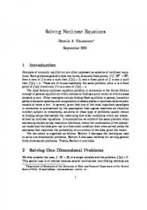
Fig. 3: (Ex.2, y3 ) line = exact solution, dashed line = standard NIM, long dashed line = revised ADM, dotted line = revised NIM
0
Ex.3: Consider system of nonlinear partial differential equations [11]:
The revised NIM leads to y1,0 = 1, y2,0 = 1, y3,0 = 0;
∂u ∂u y1,1 = 2t, y2,1 = 3 − 3e−t − 2te−t , +v + u = 1, u(x, 0) = ex , ∂t ∂x −t −t y3,1 = −5 + 4t + 5e + 2te ; ∂v ∂v −u − v = 1, v(x, 0) = e−x . (11) y1,2 = −63 + 30t + 80e−t − 4t2 e−2t − 16te−2t − 17e−2t , ∂t ∂x 196 209 −3t 56 + e y2,2 = − 48e−2t + 33e−t + te−3t The system (11) is equivalent to 27 27 9 ) ∫ t( 4 ∂u −16te−2t − 30te−t + t2 e−3t , x u = (e + t) − u+v dt, 3 ∂x 0 −395 91 −3t 61 −2t −t ( ) ∫ y3,2 = − e + 28e − 10e + t t ∂v 27 27 27 −x v = (e + t) + v+u dt. (12) 64 −3t 4 ∂x 0 − te + 8te−2t + 28te−t + 2t2 − t2 e−3t , 27 9 x−t t−x and so on. In Fig.1, Fig.2 and Fig.3 we compare the solutions The exact solution of (15) is u(x, t) = e , v(x, t) = e . Employing revised NIM to (15), we get of (10) with the solutions by standard NIM and by revised ADM [10]. Solid line shows exact solution, dotted line shows u0 = ex + t, v0 = e−x + t; solution by revised NIM, dashed line shows standard NIM −t solution and long dashed line shows revised ADM solution. u1 = (2 + t)(1 + ex ), 2 y1 ( ) t v1 = e−x 6 + t2 + ex (−6 + 6t + t2 ) ; 6 50 and so on. In Fig.4, Fig.5, Fig.6 and Fig.7 we draw 3-term solutions and exact solutions of (11), it is clear from figures that the 3-term solutions are in agreement with the exact solutions.
40 30 20 10 1
0.5
1.5
2
Fig. 1: (Ex.2, y1 ) y2
t
Ex.4: Consider system representing nonlinear chemical reaction [12] y1
′
= −y1 ,
′
y2
= y1 −
′
7
y3
6 5 4 3 2 1 0.5
1
1.5
Fig. 2: (Ex.2,y2 )
2
t
=
y22 ,
y1 (0) = 1, y22 ,
y2 (0) = 0,
y3 (0) = 0.
The system (13) is equivalent to ∫ t y1 = 1 − y1 dt; 0 ∫ t ∫ t y2 = y1 dt − y22 dt; 0 0 ∫ t y3 = y22 dt. 0
(13)
Applying revised NIM, we get
10 v
0.4
5
y1,0 = 1, y2,0 = 0, y3,0 = 0; −t t3 y1,1 = −t, y2,1 = (t − 2), y3,1 = (20 − 15t + 3t2 ); 2 60 t2 t3 y1,2 = , y2,2 = (10 − 15t + 3t2 ), 2 60 t5 y3,2 = (−55440 + 92400t − 38280t2 − 3465t3 831600 +7315t4 − 2079t5 + 189t6 ),
0.2 0 -2
0 t -0.2
-1 0 x
1
-0.4 2
Fig. 6: (Ex.3, 3-term solution v)
··· .
Fig.8, Fig.9 and Fig.10 represents the 3-term solutions of (13). Note that these graphs are in agreement with the graphs given in [12].
10 v
0.4
5
0.2
0 -2
0 t -0.2
-1 0 x
1
-0.4 2
Fig. 7: (Ex.3, Exact solution v = et−x ) 10 u
0.4
5
0.2 0 -2
0 t -0.2
-1 0 x
1
y1 t 0.00020.00040.00060.0008 0.001 0.9998 0.9996
-0.4 2
0.9994
Fig. 4: (Ex.3, 3-term solution u)
0.9992 0.999
Fig. 8: (Ex.4, 3-term solution y1 ) y2 0.001 10 u
0.4
5
0.2 0 -2
0 t -0.2
-1 0 x
0.0008 0.0006 0.0004 0.0002
1
-0.4 2
Fig. 5: (Ex.3, Exact solution u = ex−t )
t 0.00020.00040.00060.0008 0.001
Fig. 9: (Ex.4, 3-term solution y2 )
tial equations
y3 -10
2·10
-10
1.5·10
Dtα y1
= −y1 + y2 y3 ,
Dtα y2 Dtα y3
= −y2 y3 − y2 (0) = 2, 2 = y2 , y3 (0) = 0, 0 < α ≤ 1.
y1 (0) = 1,
2y22 ,
(16)
-10
1·10
Applying (3), we get equivalent system of integral equations -11
5·10
y1 y2
t 0.00020.00040.00060.00080.001
y3
Fig. 10: (Ex.4, 3-term solution y3 )
In view of revised NIM, y1,0 = 1, y2,0 = 0, y3,0 = 0; tα y1,1 = − , Γ(α + 1) 8tα y2,1 = − , Γ(α + 1) ( ) √ 4tα 42+α t2α Γ(α + 0.5) 23−2α πtα y3,1 = + √ 1− , Γ(α + 1) Γ(α + 0.5) πΓ(1 + 3α)
5 4
y2 y1
3 2 1 0.2 0.4 0.6 0.8
1
and so on.
t
1.2 1.4
VI. C ONCLUSIONS
Fig. 11: (Ex.5, 4-term solutions) Ex.5: Consider the system of nonlinear fractional differential equations Dt1.3 y1
= y1 + y22 ,
Dt2.4 y2
= y1 + 5y2 ,
′
y1 (0) = 0, y1 (0) = 1, ′
′′
y2 (0) = 0, y2 (0) = y2 (0) = 1. (14)
In view of (3), this system is equivalent to the following system of equations y1
= t+
y2
= t+
It1.3 2
t + It2.4 (y1 + 5y2 ) . 2
In this article a modification of NIM, termed as ’revised NIM’ has been presented. It has been applied successfully to solve a variety of problems formulated in terms of systems of functional equations. Revised NIM gives series solution which converges faster relative to the series obtained by NIM. The solutions obtained are highly in agreement with the exact solutions. ACKNOWLEDGMENT V. Daftardar-Gejji acknowledges the Department of Science and Technology, N. Delhi, India for the Research Grants [Project No SR/S2/HEP-024/2009].
( ) y1 + y22 ; (15)
Applying revised NIM to (15) we get t2 ; 2 = 0.372656t2.3 + 0.225852t3.3
y1,0 = t, y2,0 = t + y1,1
1 + Itα (−y1 + y2 y3 ) ; ( ) = 2 + Itα −y2 y3 − 2y22 ; ( ) = Itα y22 .
=
+0.157571t4.3 + 0.0297305t5.3 , y2,1 = 0.591944t3.4 + 0.1121t4.4 + 0.01379t4.7 +0.004838t5.7 + 0.002166t6.7 + 0.000281t7.7 ; y1,2 = 0.0747312t3.6 + 0.0324918t4.6 + · · · + 3.44154 × 10⁻⁸ t15.7 + 2.0608 × 10⁻⁹ t16.7 , y2,2 = 0.0604101t5.8 + 0.00138889t6 + · · · +3.63177 × 10⁻¹¹ t18.1 + 1.90145 × 10⁻¹² t19.1 , and so on. Fig.11 represents the 4-term approximate solutions of (14). Ex.6: Consider the system of nonlinear fractional differen-
R EFERENCES [1] I. Podlubny, Fractional Differential Equations, Academic Press, San Diego, 1999. [2] L. Debnath, Int. J. Math. and Math. Sci., 2003, 1(2003) [3] G. Adomian, Solving Frontier Problems of Physics: The Decomposition Method, Kluwer, 1994. [4] J. H. He, Comput. Meth. Appl. Mech. Eng., 167, 57(1998) [5] J. H. He, Comput. Meth. Appl. Mech. Eng., 178, 257(1999) [6] V. Daftardar-Gejji, H. Jafari, J. Math. Anal. Appl., 316, 753(2006) [7] S. Bhalekar, V. Daftardar-Gejji, Solving Riccati differential equations of fractional order using the new iterative method, (submitted for publication). [8] S. Bhalekar, V. Daftardar-Gejji, New Iterative Method: Application to Partial Differential Equations, (submitted for publication). [9] S. G. Samko, A. A. Kilbas, O. I. Marichev, Fractional Integrals and Derivatives: Theory and Applications, Gordon and Breach, Yverdon, 1993. [10] H. Jafari, V. Daftardar-Gejji, Appl. Math. Comput., 181, 598(2006) [11] A. M. Wazwaz, Comput. Math. Appl., 54, 895(2007) [12] D.D. Ganji, M. Nourollahi, E. Mohseni, Comput. and Math. with Appl., (In press), doi:10.1016/j.camwa.2006.12.078.