Mar 4, 2017 - architecture and they compose the input, hidden and output layers. ..... of 1,965 face images of. 1http://www.cs.nyu.edu/Ëroweis/data.html ...
Matrix-Centric Neural Nets
arXiv:1703.01454v1 [cs.LG] 4 Mar 2017
Kien Do, Truyen Tran, Svetha Venkatesh Centre for Pattern Recognition and Data Analytics Deakin University, Geelong, Australia {dkdo, truyen.tran, svetha.venkatesh}@deakin.edu.au
Abstract We present a new distributed representation in deep neural nets wherein the information is represented in native form as a matrix. This differs from current neural architectures that rely on vector representations. We consider matrices as central to the architecture and they compose the input, hidden and output layers. The model representation is more compact and elegant – the number of parameters grows only with the largest dimension of the incoming layer rather than the number of hidden units. We derive feed-forward nets that map an input matrix into an output matrix, and recurrent nets which map a sequence of input matrices into a sequence of output matrices. Experiments on handwritten digits recognition, face reconstruction, sequence to sequence learning and EEG classification demonstrate the efficacy and compactness of the matrix-centric architectures.
1
Introduction
Recent advances in deep learning have generated a constant stream of new neural architectures, ranging from variants of feed-forward nets to differentiable Turing machines [LeCun et al., 2015; Graves et al., 2016]. Nevertheless, the central components of these nets are still reliant on vector representations due to simplicity in mathematical modeling and programming. For domains where data are naturally represented in matrices, for example, images or multi-channel signals, the vector representation is sub-optimal because of two reasons. First, it requires vectorization by stretching all columns into a single vector – this operation destroys the intrinsic multi-mode structure. Second, failing to account for the relations between data modes usually leads to a larger model whose parameters grow with the number of matrix cells. To overcome these drawbacks, we present a new notion of distributed representation for matrix data wherein the input, hidden and output layers are matrices. The connection between an input and an output layer is a nonlinear matrix-matrix mapping parameterized by two other parameter matrices, one that captures the correlation between rows, and the other captures the correlation between columns. It results in a powerful yet highly compact model that is not only able to represent
the structure of a matrix but also has a parameter growth rate that equals the largest dimension of the matrix. We have discovered an attractive feature of the matrixmatrix mapping in that it allows us to build deep matrix networks, circumventing this problem with equivalent vector representations. It acts as a kind of regularization to the matrix structure, and we term it structural regularization. Furthermore, all neural networks that use conventional vector representations can be replaced with the matrix counterparts we propose, creating new matrix-centric neural nets. We demonstrate the application of our techniques for feed-forward networks, recurrent networks and finally convolutional networks. For recurrent nets, each time step has a matrix memory where rows/columns can be considered as memory slots and matrix mapping works like the attentive reading operator in [Graves et al., 2014]. Convolutional nets [LeCun et al., 1995] whose output is typically a set of 2D feature maps can be combined seamlessly with matrix-centric networks using tensor-matrix mapping, and this preserves spatial structure of feature maps. We evaluate our methods on four diverse experiments. The first uses feed-forward nets for handwritten digit recognition. The second problem is face reconstruction from occlusion using auto-encoders. In these two experiments, we carefully examine the structural regularization effect. Next is a sequenceto-sequence learning task wherein we test the performance of matrix recurrent nets. Finally, for classification of EEG signals, we integrate CNNs used as feature extractors with matrix LSTMs to model the temporal dynamics of frequencies along different channels. To summarize, our main contributions are: • Introduction of a novel neural net approach that incorporates matrices as the basic representation; • Hypothesis about a regularization mechanism related to the matrix mapping for such architectures; • Derivation of new matrix representation alternative for the two canonical architectures: feed-forward nets and recurrent nets. We also propose a method to convert the output of convolutional layers into a matrix, which can then be used in matrix feed-forward nets or recurrent nets; • Demonstration of the efficacy of matrix-centric neural nets on a comprehensive suite of experiments.
2
Methods
We present our main contribution, the matrix-centric neural architectures.
2.1
Matrix-Matrix Mapping
With conventional vector representation, the mapping from an input vector x to an output vector y has the form y = σ(W x + b) where b is a bias vector, W is a mapping matrix and σ is an element-wise nonlinear transformation. Likewise, in our new matrix representation, the building block is a mapping from an input matrix X of size c1 × r1 to an output matrix Y of size c2 × r2 , as follows: Y
=
σ(U | XV + B)
(1)
where U ∈ Rc1 ×c2 is the row mapping matrix, V ∈ Rr1 ×r2 is the column mapping matrix and B ∈ Rc2 ×r2 is the bias matrix. With this mapping, building a deep feedforward network is straightforward by stacking the matrix-matrix layers on top of each other. Eq. (1) has interesting properties. First, the number of parameter scales linearly with only the largest dimension of input/output matrices with c1 c2 + r1 r2 + c2 r2 parameters. For conventional vector representation, we would need c1 c2 r1 r2 + c2 r2 parameters. Second, the representation in Eq. (1) is indeed a low-rank factorization of the mapping matrix in the case of full vector representation, which we will show next.
2.2
c1 × r1 . Eq. (4) shows that the weights U:,i and V:,j that map the whole input matrix X to an output element Yi,j is the low-rank decomposition of the dense weights W:,i×r2 +j used in equivalent vector mapping. .
2.3
mat(X, H; θ)
yk
=
σ
| W:,k x
+ bk
� !
=
σ
X
(W:,k x) + bk
(2)
all elements
On the other hand, we can slightly modify Eq. (1) to describe the mapping from the entire matrix X to an element Yi,j of the matrix Y :
In case of matrix Long Short-Term Memory (matrixLSTM), the formula of a block (without peep-hole connection) at time step t can be specified as follows: It Ft Ot Cˆt
Yi,j
= σ = σ
X
+ Bij
� !
| (U:,i V:,j all elements
X) + Bij
(3)
If we refer yk and Yi,j to be the same component, e.g. k = i × r2 + j, Eq. (2) and Eq. (3) must be equal. Then we have: matrix(W:,i×r2 +j )
| = U:,i V:,j
(4)
where matrix(W;i×r2 +j ) means that the column vector W;i×r2 +j of length c1 r1 is reshaped to a matrix of shape
= σ(mat(Xt , Ht−1 ; θ i )) = σ(mat(Xt , Ht−1 ; θ f )) = σ(mat(Xt , Ht−1 ; θ o )) =
tanh(mat(Xt , Ht−1 ; θ c )) = Ft Ct−1 + It Cˆt = Ot tanh(Ct )
where denotes the Hadamard product; and It , Ft Ot , Cˆt are input gate, forget gate, output gate and cell gate at time t, respectively. Note that the memory cells Ct that store, forget and update information is a matrix. Remark: The second term Uh| HVh in Eq. (5) bears some similarity with the external memory bank in a Neural Turing Machine [Graves et al., 2014; Graves et al., 2016]. The state matrix H can be viewed as an array of memory slots while each i-th column vector of the matrix Uh| acts as (unnormalized) attention weights to select which rows of H to read from and each j-th row of the matrix Vh specifies which parts of a memory slot are most informative.
2.4 | U:,i XV:,j
(5)
Ht = σ (mat (Xt , Ht−1 ; θ i ))
Ct Ht
Assume that we vectorize X and Y into vector x of length c1 r1 and y of length c2 r2 , respectively and use standard vectorvector mapping between them: y = σ(W | x + b) where W is the parameter matrix of shape c1 r1 ×c2 r2 . Thus, each element yk with k ∈ {1, ..., c2 r2 } can be computed as follows:
:= Ux| XVx + Uh| HVh + B
where θ = {Ux , Vx , Uh , Vh , B}. The next state in vanilla matrix-RNNs is simply:
Matrix-Matrix Mapping as Low-Rank Factorization
�
Matrix Recurrent Networks
We now present the matrix extension of recurrent networks. Here, the input, output and hidden state at each time step are matrices. For ease of development, let us introduce the notation mat(X, H; θ), defined as:
Tensor-Matrix Mapping
For spatial inputs, convolutional layers are essential to learn translation-invariant features. The output of a convolutional layer is usually a set of 2D feature maps – or in other words, a 3D tensor. The matrix neural nets defined above can easily connect to CNNs using a tensor-matrix mapping. Since these feature maps are structured, flattening them into vectors as in conventional CNNs may loose information. We propose to treat these 2D maps as matrices. Denote X as the output of the convolutional layer. X is a 3D tensor of shape (m, c1 , r1 ) where m is the number of feature maps, each has shape c1 × r1 . We want to map this tensor to a 2D matrix Y of shape (c2 , r2 ). To do so, we use two 3D tensors U and V of shape (m, c1 , c2 ) and (m, r1 , r2 )
0.5
matrix-(20, 20) matrix-(50, 50) vector-50 vector-100 vector-200
0.4
error
0.3
0.2
Figure 1: Tensor-matrix mapping, where X is the tensor output of the convolutional layer, Y is the desired matrix representam tion, and {Ui , Vi }i=1 are mapping parameters.
0.1
0.0
respectively as parameters. Then the tensor-matrix mapping is defined as:
Y
=
m X
Ui| Xi Vi
5
10
15
depths
20
25
30
Figure 2: Test errors of matrix and vector feed-forward nets over MNIST with depth varying from 5 to 30. Nets trained without Batch-Norm. Best viewed in color.
(6)
i=1
See Fig. 1 for a graphical illustration. With this mapping, CNNs can naturally serve as a feature detector for matrixcentric neural nets in spatial domains.
3
Experiments
In this section, we experimentally validate the proposed matrixcentric architectures described in Section. 2. For all experiments presented below, our networks use ReLU activation function and are trained using Adam [Kingma and Ba, 2014].
1.0 0.8 0.6 0.4 0.2 0.0 1.0 0.8 0.6 0.4 0.2 0.0
train
0
50
100 150 200 0
50
valid
100 150 2000
50
100 150 200
0.9 0.8 0.7 0.6 0.5 0.4 0.3 0.2 0.1 0.0 0.9 0.8 0.7 0.6 0.5 0.4 0.3 0.2 0.1 0.0
(a) Vector nets
3.1
0
50
100 150 200
(b) Matrix nets
Feedforward Nets on MNIST
The MNIST dataset consists of 70K handwritten digits of size 28 × 28, with 50K images for training, 10K for testing and 10K for validation. For matrix nets, images are naturally matrices, but for traditional vector nets, images are vectorized into vectors of length 784. To test the ability to accommodate very deep nets without skip-connections [Srivastava et al., 2015b; Pham et al., 2016], we create vector and matrix feed-forward nets with increasing depths. The top layers are softmax as usual for both vector and matrix nets. We compare matrix nets with the hidden shape of 20 × 20 and 50 × 50 against vector nets containing 50, 100 and 200 hidden units. We observe that without Batch-Norm (BN) [Ioffe and Szegedy, 2015], vector nets struggle to learn when the depth goes beyond 20, as evidenced in Fig. 2. The erratic learning curves of the vector nets at depth 30 are shown in Fig. 3a, top row. With the help of BN layers, the vector nets can learn normally at depth 30 (see the test errors in Fig. 2), but again fail beyond depth 50 (see Fig. 3a, bottom row). The matrix nets are far better: They learn smoothly at depth 30 without BN layers (Fig. 3b, top). With BN layers, they still learn well at depth 50 (Fig. 3b, bottom) and can manage to learn up to depth 70 (result is not shown here). These behaviors suggest that matrix nets might exhibit a form structural regularization that simplifies the loss surface, which is the subject for future investigation (e.g., see [Choromanska et al., 2015] for an account of vector nets).
Figure 3: Learning curves of vector and matrix feed-forward nets over MNIST. (a) Left to right: Vector nets with 50, 100, 200 hidden units. (b): Matrix nets with 50 × 50 hidden units. Top: 30-layer nets without Batch Norm. Bottom: 50-layer nets with Batch Norm. We visualize the weights of the first layer of the matrix net with hidden layers of 50 × 50 (the weights for 20 × 20 layers are similar) in Fig. 4 for a better understanding. In the plots of U and V (top and bottom left of Fig. 4, respectively), the short vertical brushes indicate that some adjacent input features are highly correlated along the row or column axes. For example, the digit 1 has white pixels along its line which will be captured by U . In case of W , each square tile in Fig. 4(right) corresponds to the weights that map the entire input matrix to a particular element of the output matrix. These weights have cross-line patterns, which differ from stroke-like patterns commonly seen in vector nets.
3.2
Autoencoders for Corrupted Face Reconstruction
To evaluate the ability of learning structural information in images of matrix-centric nets, we conduct experiments on the Frey Face dataset1 , which consists of 1,965 face images of 1
http://www.cs.nyu.edu/˜roweis/data.html
0.8 0.6 0.4 0.2 0.0 0.2 0.4 0.6
Figure 4: The normalized weights of the first layer of the 30-layer matrix feed-forward net with hidden size of 50 × 50 trained on MNIST. Weights of other layers look quite similar. Top left: Row mapping matrix U of shape 28 × 50. Bottom left: Column mapping matrix V of shape 28 × 50. Right: Each square tile i, j show the weight W:,i×50+j which is the outer product of U:,i and V:,j . size 28 × 20, taken from sequential frames of a video. We randomly select 70% data for training, 20% for testing and 10% for validation. Test images are corrupted with 5 × 5 black square patches at random positions. Auto-encoders (AEs) are used for this reconstruction task. We build deep AEs consisting of 20 and 40 layers. For each depth, we select vector nets with 50, 100, 200 and 500 hidden units and matrix nets with hidden shape of 20 × 20, 50 × 50, 100 × 100 and 150 × 150. The encoders and the decoders have tied weights. The AEs are trained with backprop, random noise added to the input with ratio of 0.2, and L1 and L2 regularizers. Once trained, AEs are used to reconstruct the test images. Fig. 5 presents several reconstruction results. Vector AEs fail to learn to reconstruct either with or without weight regularization. Without weight regularization, vector AEs fail to remove noise from the training images (Fig. 5b), while with weight regularization they collapse to a single mode (Fig. 5b)2 . Matrix AEs, in contrast, can reconstruct the test images quite well without weight regularization (see Fig. 5d). In fact, adding weight regularization to matrix AEs actually deteriorates the performance, as shown in Figs. 5(e,f). This suggests a couple of conjectures. One is there exists structural regularization in matrix-centric nets (e.g., due to the implicit weight matrixfactorization shown in Section. 2.2), hence weight regularization is not needed. The other is that matrix-like structures in images are preserved in matrix-centric nets, enabling missing information to be recovered.
3.3
Sequence to Sequence Learning with Moving MNIST
In this experiment, we compare the performance of matrix and vector recurrent nets in a sequence-to-sequence (seq2seq) learning task [Sutskever et al., 2014; Srivastava et al., 2015a]. We choose the Moving MNIST dataset3 which contains 10K image sequences. Each sequence has length of 20 showing 2 digits moving in 64 × 64 frames. We randomly divide the 2 This happens for all hidden sizes and all depth values of vector AEs specified above. 3 http://www.cs.toronto.edu/˜nitish/unsupervised video/
dataset into 6K, 3K and 1K image sequences with respect to training, testing and validation. In our seq2seq model, the encoder and the decoder are both recurrent nets. The encoder captures information of the first 15 frames while the decoder predicts the last 5 frames using the hidden context learnt by the encoder. Different from [Srivastava et al., 2015a], the decoder do not have readout connections4 for simplicity. We build vector seq2seq models with hidden sizes ranging from 100 to 2000 for both the encoder and the decoder. In case of matrix seq2seq models, we choose hidden sizes from from 10 × 10 to 200 × 200. Later in this section, we write vector RNN/LSTM to refer to a vector seq2seq model with the encoder and decoder are RNNs/LSTMs. The same notation applies to matrix. It is important to emphasize that matrix-centric nets are far more compact than the vector-centric counterparts. For example, the vector RNNs require nearly 30M parameters for 2K hidden units while the matrix RNNs only need about 400K parameters (roughly 75 times fewer) but have 40K hidden units (20 times larger)5 . The parameter inflation exhibits a huge redundancy in vector representation which makes the vector nets susceptible to overfitting. Therefore, after a certain threshold (200 in this case), increasing the hidden size of a vector RNN/LSTM will deteriorate its performance. Matrix nets, in contrast, are consistently better when the hidden shape becomes larger, suggesting that overfitting is not a problem. Remarkably, a matrix RNN/LSTM with hidden shape of 50 × 50 is enough to outperform vector RNNs/LSTMs of any size with or without dropout (see Fig. 6). Dropout does improve the representations of both vector and matrix nets but it cannot eliminate the overfitting on the big vector nets.
3.4
Sequence Classification with EEG
We use the Alcoholic EEG dataset6 of 122 subjects divided into two groups: alcoholic and control groups. Each subject completed about 100 trials and the data contains about 12K trials in total. For each trial, the subject was presented with three different types of stimuli in 1 second. EEG signals have 64 channels sampled at the rate of 256 Hz. Thus, each trial consists of 64 × 256 samples in total. We convert the signals into spectrograms using Short-Time Fourier Transform (STFT) with Hamming window of length 64 and 56 overlapping samples. The signals were detrended by removing mean values along the time axis. Because the signals are real-valued, we only take half of the frequency bins. We also exclude the first bin which corresponds to zero frequency. This results in a tensor of shape 64 × 32 × 25 where the dimensions are channel, frequency and time, respectively. Fig. 7 shows examples of the input spectrogram of an alcoholic subject in 4 channels which reveals some spatial correlations across channels and frequencies. For this dataset, we randomly separate the trials of each subject with a proportion of 0.6/0.2/0.2 for training/testing/validation. 4 the predicted output of the decoder at one time step will be used as input at the next time step 5 For LSTMs, the number of parameters quadruples but the relative compactness between vector and matrix-centric nets remain the same. 6 https://kdd.ics.uci.edu/databases/eeg/eeg.data.html
(a)
(b)
(c)
(d)
(e)
(f)
Figure 5: Images reconstructed by matrix AEs and vector AEs in comparison with ground truth. All AEs from (b) to (e) have 40 layers while the AEs at (f) have 20 layers. (a): corrupted inputs and ground truth; (b): vector AEs (hidden size of 50 and 500) without regularization; (c): vector AEs with regularization; (d): matrix AEs (hidden size of 20 × 20, 50 × 50 and 150 × 150) without regularization; (e): matrix AEs with L1 regularization; (f): matrix AEs (hidden size of 50 × 50 and 150 × 150) with L2 regularization. matrix-RNN matrix-RNN-DO matrix-LSTM matrix-LSTM-DO vector-RNN vector-RNN-DO vector-LSTM vector-LSTM-DO
94 92
loss
90 88 86 84
Channel 16
Channel 32
Channel 48
Channel 54
0.0 16.0 32.0
Frequency (Hz)
96
48.0 64.0 80.0 96.0
112.0 128.0
0
5
10
15
20
0
5
10
15
20
0
Time
5
10
15
20
0
5
10
15
20
Figure 7: Spectrograms of four channels taken from one trial of a random alcoholic subject. Best viewed in color.
82 80 78
0
5000
10000
15000
20000
25000
hidden units
30000
35000
40000
Figure 6: Reconstruction loss over test data of matrix and vector seq2seq models as functions of hidden unit. DO is short for Dropout which is set at 0.2 for inputs and 0.5 for hidden units. Best viewed in color.
To model the frequency change of all channels over time, we use LSTMs [Hochreiter and Schmidhuber, 1997]. We choose vector LSTMs with 200 hidden units which show to work best in the experiment with Moving MNIST. For matrix LSTMs, we select the one with hidden shape of 100 × 100. We evaluate six different settings for this task. Models 1 and 2 both receive plain spectrogram inputs which are sequences of matrices of shape 64 × 32. In case of Model 1, these matrices are flattened into vectors. Models 3, 4, 5, 6 use an additional spatial feature detector which is a 2-conv (short for convolutional) layer CNN. The first conv layer uses 32 filters of shape 5 × 5 while the second conv layer uses 64 filters of shape 3 × 3. Each conv
layer is followed by a 2 × 2 subsampling layer. Hence, the output of this CNN model is a tensor of shape 64 × 14 × 6. For Model 3, we add a global conv layer (denoted as CNN-g in Tab. 1) with 200 filters of shape 14 × 6 above the CNN and get an output vector of length 200. We feed this vector to the vector LSTM. For Model 5, we reshape the 64 × 14 × 6 tensor into a 64 × 84 matrix (CNN-s) and feed it to the matrix LSTM. Models 4 and 6 employ the tensor-matrix mapping described in Section. 2.4 to convert this tensor into a matrix of shape 50 × 50 (CNN-m), which is fed to the vector LSTM (after vectorization) and the matrix LSTM, respectively. As seen in Tab. 1, the vector LSTM with raw input (Model 1) not only achieves the worst result but also consumes a very large number of parameters. The plain matrix LSTM (Model 2) improves the result by a large margin (about 3.5%) while having far fewer parameters than of Model 1. When the CNN feature detector is presented (in Models 3 and 4), the errors for the vector LSTMs drop dramatically, suggesting that spatial representation is important for this type of data. However, even with the help of conv layers, the vector LSTMs are not able to compete against the plain matrix LSTM.
Model vec-LSTM (1) mat-LSTM (2) CNN-g + vec-LSTM (3) CNN-m + vec-LSTM (4) CNN-s + mat-LSTM (5) CNN-m + mat-LSTM (6)
# Params 1,844,201 160,601 1,435,729 2,266,829 200,729 248,029
Err (%) 5.29 1.71 1.90 2.63 4.12 1.44
Table 1: Classification accuracy and number of parameters of different models. CNN-g: global vectorization of CNN output, CNN-m: tensor-matrix mapping of CNN output, CNN-s = simple reshaping by vectorization per channel of the CNN output. Similar to vector LSTMs, we can use the CNN to detect feature maps for matrix LSTMs. However, if we just simply reshape the output of the CNN as being done in Model 5, the result will be poorer. This is because the reshaping destroys the 2D information of each feature map. On the other hand, with proper tensor-matrix mapping (see Section 2.4) where the 2D structure is preserved, matrix LSTM (Model 6) yields the best result of 1.44% error, which compares favorably to the best result achieved by the vector LSTMs (1.90%). Importantly, this matrix LSTM requires 6 times less parameters than its vector counterpart.
4
Related Work
Matrix data modeling has been well studied in shallow or linear settings, such as 2DPCA [Yang et al., 2004], 2DLDA [Ye et al., 2004], Matrix-variate Factor Analysis [Xie et al., 2008], Tensor analyzer [Tang et al., 2013], Matrix/tensor RBM [Nguyen et al., 2015; Qi et al., 2016]. Except 2DPCA and 2DLDA, all other methods are probabilistic models which use matrix mapping to parameterize the conditional distribution of the observed random variable given the latent variable. However, since these models are shallow, their applications of matrix mapping are limited. Our work inherits the matrix mapping idea from these models and extends it to a wide range of deep neural networks. There have been several original deep architectures recently proposed to handle multidimensional data such as Multidimensional RNNs [Graves and Schmidhuber, 2009], Grid LSTMs [Kalchbrenner et al., 2015] and Convolutional LSTMs [Xingjian et al., 2015]. The main idea of the first two models is that any spatial dimension can be considered as a temporal dimension. They extend the standard recurrent networks by making as many new recurrent connections as the dimensionality of the data. These connections allow the network to create a flexible internal representation of the surrounding context. Although Multidimensional RNNs and Grid LSTMs are shown to work well with many high dimensional datasets, they are complicate to implement and have a very long recurrent loop (often equal to the input tensor’s shape) run sequentially. A convolutional LSTM, on the other hand, works like a standard recurrent net except that its gates, memory cells and hidden states are all 3D tensors with convolution as the mapping operator. Consequently, each local region in the hidden memory is attended and updated over time. This is different from our
model since a matrix recurrent net attends to every row/column vector of its hidden memory. We are also aware of another work [Novikov et al., 2015] that proposes matrix decomposition of the weight matrix in vector-vector mapping similar to ours. They show that this kind of matrix decomposition is, indeed, a specific case of a more general Tensor Train (TT) transformation [Oseledets, 2011] when the tensor is a 2D matrix. However, their work solely focuses on model compression using the TT transformation for feed-forward nets7 . Our main contributions are creating a matrix-centric ecosystem of neural nets, which include feed-forward, recurrent and convolutional architectures. RNNs with augmented memory and attention present an implicit use of matrix modeling: each row is a piece of memory and the entire memory is a matrix (e.g., those in NTM [Graves et al., 2014; Graves et al., 2016] and Memory Networks [Weston et al., 2014]). Reading and writing require attention to a specific memory piece. However, most attention schemes maintain a softmax distribution over all memory pieces to maintain differentiability. The attention distribution is like the row-mapping matrix in our case.
5
Discussion
We have introduced a new notion of distributed representation in neural nets where information is distributed across neurons arranged in a matrix. This departs from the existing representation using vectors. Matrix-centric representation is in line with recent memory-augmented RNNs, where external memory is an array of memory slots – essentially a matrix arrangement. However, in our treatment, matrices are first-class citizen: neurons in a layer are always arranged in a matrix. We derive matrix-centric feedforward and recurrent nets, and propose a method to convert convolutional outputs into a matrix. We theoretically show that through matrix factorization of weights, a traditional vector net can be replaced by an equivalent matrix net when modeling matrix data. This results in much a more compact matrix-centric net, and benefits from structural regularization. We evaluate our proposed neural architectures on four applications: handwritten digit recognition (MNIST), face reconstruction under block occlusion, sequence-to-sequence prediction of moving digits, and EEG classification. The experiments have demonstrated that matrix-centric nets are highly compact and perform better than vector-centric counterparts when data are inherently matrices. Matrix-centric representation opens a wide room for future work. Structural regularization, the loss surfaces and the connection with memory-augmented RNNs deserve more deep investigations. It might also be useful to design matrix-centric CNNs, where the receptive fields can be factorized via the matrix-matrix mapping. Further, as matrix is an effective representation for graphs, it remains open to apply matrix-centric nets in these domains.
References [Choromanska et al., 2015] Anna Choromanska, Mikael Henaff, Michael Mathieu, G´erard Ben Arous, and Yann 7 They do use CNNs in their paper but only the top fully-connected layers are modified with TT transformation
LeCun. The loss surfaces of multilayer networks. In AISTATS, 2015. [Graves and Schmidhuber, 2009] Alex Graves and J¨urgen Schmidhuber. Offline handwriting recognition with multidimensional recurrent neural networks. In Advances in neural information processing systems, pages 545–552, 2009. [Graves et al., 2014] Alex Graves, Greg Wayne, and Ivo Danihelka. Neural turing machines. arXiv preprint arXiv:1410.5401, 2014. [Graves et al., 2016] Alex Graves, Greg Wayne, Malcolm Reynolds, Tim Harley, Ivo Danihelka, Agnieszka GrabskaBarwi´nska, Sergio G´omez Colmenarejo, Edward Grefenstette, Tiago Ramalho, John Agapiou, et al. Hybrid computing using a neural network with dynamic external memory. Nature, 538(7626):471–476, 2016. [Hochreiter and Schmidhuber, 1997] Sepp Hochreiter and J¨urgen Schmidhuber. Long short-term memory. Neural computation, 9(8):1735–1780, 1997. [Ioffe and Szegedy, 2015] Sergey Ioffe and Christian Szegedy. Batch normalization: Accelerating deep network training by reducing internal covariate shift. arXiv preprint arXiv:1502.03167, 2015. [Kalchbrenner et al., 2015] Nal Kalchbrenner, Ivo Danihelka, and Alex Graves. Grid long short-term memory. arXiv preprint arXiv:1507.01526, 2015. [Kingma and Ba, 2014] Diederik Kingma and Jimmy Ba. Adam: A method for stochastic optimization. arXiv preprint arXiv:1412.6980, 2014. [LeCun et al., 1995] Yann LeCun, Yoshua Bengio, et al. Convolutional networks for images, speech, and time series. The handbook of brain theory and neural networks, 3361(10):1995, 1995. [LeCun et al., 2015] Yann LeCun, Yoshua Bengio, and Geoffrey Hinton. Deep learning. Nature, 521(7553):436–444, 2015. [Nguyen et al., 2015] Tu Dinh Nguyen, Truyen Tran, Dinh Q Phung, and Svetha Venkatesh. Tensor-variate restricted boltzmann machines. In AAAI, pages 2887–2893, 2015. [Novikov et al., 2015] Alexander Novikov, Dmitrii Podoprikhin, Anton Osokin, and Dmitry P Vetrov. Tensorizing neural networks. In Advances in Neural Information Processing Systems, pages 442–450, 2015. [Oseledets, 2011] Ivan V Oseledets. Tensor-train decomposition. SIAM Journal on Scientific Computing, 33(5):2295– 2317, 2011.
[Pham et al., 2016] Trang Pham, Truyen Tran, Dinh Phung, and Svetha Venkatesh. Faster training of very deep networks via p-norm gates. ICPR, 2016. [Qi et al., 2016] Guanglei Qi, Yanfeng Sun, Junbin Gao, Yongli Hu, and Jinghua Li. Matrix variate restricted boltzmann machine. In Neural Networks (IJCNN), 2016 International Joint Conference on, pages 389–395. IEEE, 2016. [Srivastava et al., 2015a] Nitish Srivastava, Elman Mansimov, and Ruslan Salakhutdinov. Unsupervised learning of video representations using lstms. arXiv preprint arXiv:1502.04681, 2015. [Srivastava et al., 2015b] Rupesh K Srivastava, Klaus Greff, and J¨urgen Schmidhuber. Training very deep networks. In Advances in neural information processing systems, pages 2377–2385, 2015. [Sutskever et al., 2014] Ilya Sutskever, Oriol Vinyals, and Quoc VV Le. Sequence to sequence learning with neural networks. In Advances in Neural Information Processing Systems, pages 3104–3112, 2014. [Tang et al., 2013] Yichuan Tang, Ruslan Salakhutdinov, and Geoffrey E Hinton. Tensor analyzers. In ICML (3), pages 163–171, 2013. [Weston et al., 2014] Jason Weston, Sumit Chopra, and Antoine Bordes. Memory networks. arXiv preprint arXiv:1410.3916, 2014. [Xie et al., 2008] Xianchao Xie, Shuicheng Yan, James T Kwok, and Thomas S Huang. Matrix-variate factor analysis and its applications. IEEE transactions on neural networks, 19(10):1821–1826, 2008. [Xingjian et al., 2015] SHI Xingjian, Zhourong Chen, Hao Wang, Dit-Yan Yeung, Wai-Kin Wong, and Wang-chun Woo. Convolutional lstm network: A machine learning approach for precipitation nowcasting. In Advances in Neural Information Processing Systems, pages 802–810, 2015. [Yang et al., 2004] Jian Yang, David Zhang, Alejandro F Frangi, and Jing-yu Yang. Two-dimensional PCA: a new approach to appearance-based face representation and recognition. IEEE transactions on pattern analysis and machine intelligence, 26(1):131–137, 2004. [Ye et al., 2004] Jieping Ye, Ravi Janardan, and Qi Li. Twodimensional linear discriminant analysis. In Advances in neural information processing systems, pages 1569–1576, 2004.