Engineering Letters, 24:1, EL_24_1_11 ______________________________________________________________________________________
Maximising Performance of Genetic Algorithm Solver in Matlab Son Duy Dao, Kazem Abhary, and Romeo Marian Abstract—Genetic Algorithm solver in Matlab is one of the popular commercial optimisation solvers commonly used in scientific research. Performance of the solver heavily depends on its parameters. To maximise the solver performance, this paper proposes a systematic and comprehensive approach based on Taguchi experimental design for the parameter tuning. Effectiveness of the proposed approach is demonstrated through a number of case studies. Index Terms—Genetic algorithm solver, global optimisation, parameter tuning, Taguchi experimental design
I. INTRODUCTION
G
ENETIC Algorithm (GA) is a popular optimisation algorithm, often used to solve complex large-scale optimisation problems in many fields [1-3]. GA solver in Matlab is a commercial optimisation solver based on Genetic Algorithms, which is commonly used in many scientific research communities [4-8]. Using the solver requires an objective function and corresponding constraints. To maximise the solver performance, appropriate solver parameters such as population size, fitness scaling function, selection function, elite count, crossover fraction, mutation function, crossover function, etc. need to be chosen. There are many options of the solver parameters to choose from. When using the GA solver, selecting the right parameter set is very beneficial but it is really challenging and requires a systematic approach. Literature review conducted in this study revealed that the common methods of choosing the GA solver parameters are trial-and-error and user-experience based methods. As a result, there have been a number of papers [6, 7, 9-13] where the GA solver parameters were just chosen, without explaining how. Obviously, these approaches could not choose the optimal parameter set and consequently performance of the solver could not be maximised. Another way of selecting the GA solver parameters is to use the default values such as the one by Rezk and Al-Dadah [14]. Clearly, this approach cannot maximise the solver performance because different problems have different characteristics and therefore different solver parameter sets for different problems are often required. Manuscript received: 25 September, 2015; revised: 25 February 2016 Mr Son Duy Dao, a PhD student, is with School of Engineering, University of South Australia, Australia (corresponding author to provide e-mail:
[email protected]). Prof. Kazem Abhary is with School of Engineering, University of South Australia, Australia Dr. Romeo Marian is with School of Engineering, University of South Australia, Australia
More advanced methods of tuning the GA solver parameters are so called the combined methods in which some parameters are selected by trial-and-error/userexperience based methods, some are default parameters, some are taken from available publications and others are chosen by Design of Experiment (DoE) method. Housh, Ostfeld and Shamir [15], Sindhuja et al. [16], Lai et al. [17] and Bornschlegell et al. [4] used trial-and-error/userexperience based methods and default parameters while Kadiyala, Kaur and Kumar [18] took some default parameters of the solver and chose the rest by DoE method. In addition, trial-and-error/user-experience based methods, default parameters as well as DoE method were applied by Zomorrodi et al. [19]. Finally, Debnath, Deb and Dutta [5] chose some solver parameters based on their experiences, some by DoE method and the rest by adopting from other publications. It can be seen that above combined methods are not capable of comprehensively investigating the effects of parameters on the GA solver performance because trialand-error/user-experience based methods, default parameters and parameters adopted from other sources are still involved. To overcome these limitations, this paper proposes a comprehensive systematic approach based on Taguchi Experimental Design for tuning the parameters of the GA solver in Matlab to maximise the solver performance. The rest of this paper is organised as follows. The proposed approach for the solver parameter selection is presented in Section 2. A case study used to demonstrate the robustness of the proposed approach is then provided in Section 3. Finally, conclusions are presented in Section 4. II. PROPOSED APPROACH There are nine parameters that can significantly affect the performance of the GA solver in Matlab: population size, fitness scaling function, selection function, elite count, crossover fraction, mutation function, crossover function, migration direction and hybrid function. Some of them are integer parameters such as population size, elite count, continuous parameter such as crossover fraction, and the rest are discrete ones. For the sake of simplicity, both integer and continuous parameters are referred to as continuous parameters hereafter. To maximise the solver performance, an optimal parameter set is required. To find the optimal set of the parameters, the following four-step approach is proposed.
(Advance online publication: 29 February 2016)
Engineering Letters, 24:1, EL_24_1_11 ______________________________________________________________________________________
Step 1: Generating Taguchi experimental design As large number of parameters are involved, Taguchi experimental design [20] is the best tool to employ herein. Based on the number of parameters considered and number of parameter levels available in the solver, Taguchi Orthogonal Array Design L32 (21 48) was chosen and details of the experimental design are shown in Tables 1-2. It should be noted that one parameter (migration direction) has two levels and the rest, each has four levels as shown in Table 1.
experiment response. To make a fair comparison, computing time is set exactly the same for every experiment. Step 3: Analysing the experimental data To determine the effects of the parameters on the solver performance, Minitab ANOVA analysis is used. In ANOVA analysis, according to Yang and El-Haik [20], the relative importance of an effect to the experiment response is presented by the corresponding F value; the larger, the more important. In addition, p value is used to determine whether an effect is statistically significant to the experiment response. An effect is commonly considered significant if its p value is less than 0.05. Step 4: Selecting the parameter values Based on ANOVA analysis in Step 3, the solver parameters are classified into two groups: significant and insignificant. For insignificant parameters, their levels will be selected based on the main-effect chart generated by Minitab, in which the levels associated with the highest fitness values should be chosen. For significant parameters, the rule for selecting the parameter level is still the same as the one for insignificant parameters, except for the continuous parameters. Further tuning process, using Hill Climbing technique, can be done for the continuous significant parameters to find the optimal values if users desire; otherwise, the experimental parameter levels that give the highest fitness values are chosen. The effectiveness of the proposed approach is demonstrated by a case study. III. CASE STUDIES
Step 2: Conducting the experiments After defining objective function and constraints, the solver parameters are set according to the experiment layout shown in Table 2. Each experiment should be repeated for a number of times, say five, to increase the consistency of the
3.1. Two-Dimensional Problem A two-dimensional function with multiple optima and known global optimal solution was chosen to preliminarily verify the robustness of the proposed approach. There are two reasons for choosing such kind of test function. The first one is that it is only possible to visualise the shape of fitness landscape of a test function which has less than or equal to two dimensions and this fitness landscape visualisation can allow the user to intuitively determine the difficulty of the function. The second reason is that a test function with multiple optima and known global optimal solution can help easily evaluate the true capability of the solver. To satisfy above conditions, a function expressed by Eqs. 1-3 and shown in Fig.1 was adopted from the research of Hall [21] herein. As can be seen from Fig. 1, this function is quite
(Advance online publication: 29 February 2016)
Engineering Letters, 24:1, EL_24_1_11 ______________________________________________________________________________________ “hard” for any meta-heuristic algorithm since it is more likely to get trapped in the “big” local optimum. Question now is how to solve the described case study problem efficiently and effectively.
Results and Discussions The proposed four-step approach was applied to solve the described case study problem. The experiments were conducted and data is shown in Table 3. In addition, ANOVA table and main-effect chart generated by Minitab are presented in Table 4 and Fig. 2. The p values in Table 4 indicate that parameters B, C, D, F, G and I are statistically significant to the solver performance; among them, parameters B and F are continuous. However, the authors decided not to conduct the further tuning process for these two parameters simply because their slopes in the maineffect chart, Fig. 2, are not significant. As a result, the solver parameter set for solving the case study problem was chosen as shown Table 5.
Fig. 1: Test function (adapted from [21])
(Advance online publication: 29 February 2016)
Engineering Letters, 24:1, EL_24_1_11 ______________________________________________________________________________________ well as SA solver were randomly generated to make a fair comparison. It can be seen from Table 6 that GA solver 3 has success rate of 197 out of 200 while PS solver, SA solver, GA solver 1 and GA solver 2 have success rates of 2, 59, 3 and 10 out of 200, respectively. The success probabilities of the solvers are visualised in Fig. 3. Clearly, success rate of GA solver 3 in solving the “hard” case study problem is very high (98.5%) and it is far better than others as indicated in Fig. 3.
To validate the effectiveness of the proposed approach, a number of commercial optimisation solvers in Matlab, with different parameter sets were used to solve the case study problem and their performances are reported in Table 6. There are three solvers with default parameters namely: Pattern Search (PS solver), Simulated Annealing (SA solver) and Genetic Algorithm (GA solver 1). In addition, GA solver 2 is Genetic Algorithm solver with population size of 200 and other parameters set default. Genetic Algorithm solver with parameters tuned by the proposed approach is named GA solver 3. It is noted that each solver had 30 seconds to search for the global optimal solution with fitness value of at least 1.044. In addition, initial solutions required by PS solver as
It should be noted that the authors have attempted to apply the proposed approach to solve two other test functions as shown in Figs. 4-5 and success rate of finding the global optimal solutions is always 100%. Due to space limitation, the details of the two case studies are not presented here, and the test function shown in Fig. 1 is used as an illustrated example for a “hard” problem.
(Advance online publication: 29 February 2016)
Engineering Letters, 24:1, EL_24_1_11 ______________________________________________________________________________________ function, was not used here to make a fair comparison with three optimisation algorithms available in the literature; which means that level 1 of this parameter was guaranteed to be selected. Performance of the GA solver tuned by the proposed approach in solving the four large-scale problems will be discussed in the next Section.
3.2. Large-Scale Problem To further evaluate the robustness of the proposed approach, four large-scale case study problems were considered herein. Each problem has a known global optimal solution with 15 dimensions. Details of the problems are shown in Table 7. The proposed approach was applied to tune the parameters of the GA solver for solving the four large-scale problems. The related experiment layout and data are shown in Tables 8-11 in Appendix. It is noted that for the sake of comparison with optimisation algorithms available in the literature, the termination criterion used in these four problems was the number of objective function evaluations, as indicated in Tables 8-11. After conducting ANOVA analysis, the parameter set of the GA solver for solving different problem was selected as shown in Table 12. It is noted that for the sake of simplicity, the further tuning process as mentioned in Step 4 in Section 2 was not used in selecting the parameters in Table 12. In addition, the parameter of the GA solver, namely hybrid
Results and Discussions Quality of the solutions to the four large-scale problems, obtained by four different optimisation algorithms, is shown in Table 13. Performances of the first three algorithms, i.e. Spiral Dynamic Algorithm (SDA), Bacterial Foraging Algorithm (BFA) and Hybrid Spiral-Dynamic BacteriaChemotaxis algorithm (type R) named HSDBC-R, in solving the four problems, have been published in the research of Nasir & Tokhi [22]. To make a fair comparison, the termination criterion of the GA solver in this article was set exactly the same as in the publication of Nasir & Tokhi [22], i.e. 80000 objective function evaluations as indicated in Table 13; and the GA solver, like the other algorithms, was independently run for 30 times. The quality of the obtained solutions in terms of the best fitness value (called Best), average fitness value (called Mean) and standard deviation of the fitness values (called Std.dev.) is shown in Table 13. For problem F1, all four optimisation algorithms are capable of finding a solution which is very close to the global solution. In other words, the performances of the four algorithms in solving problem F1 are about the same. For problems F2-F4, the GA solver in this article outperforms the other optimisation algorithms available in the literature. More specifically, the GA solver always found the global solution to problem F2, with fitness value of 0.00 in 30 independent runs; while fitness values, on average, obtained by SDA, BFA and HSDBC-R are 2.76, 17.22 and 0.47, respectively. It should be noted that all four problems herein are minimum optimisation problems. The results in Table 13 reveal that problems F3-F4 seem to be harder than problems F1-F2, since none of the four algorithms could find solutions which are very close to the global solutions. However, on average, the solution to problem F3, obtained by the GA solver in this article, is 97.2, 75.3 and 41.0% better, compared to those obtained by SDA, BFA and HSDBC-R, respectively; for problem F4, these figures are 86.5, 89.4 and 83.0%, respectively. In terms of consistency, the GA solver in this article is also better than SDA, BFA and HSDBC-R, as shown in Table 13. IV. CONCLUSION In this paper, a systematic and comprehensive approach based on Taguchi experimental design has been proposed to support users of Matlab GA solver in selecting the solver parameters to maximise its performance. The effectiveness of the proposed approach has been demonstrated through a “hard” two-dimensional problem in which the success rate of finding the global optimal solution of the GA solver with parameters tuned by the proposed approach was 98.5%, in comparison with the rates of 1.5 and 5.0% of the two conventional GA solvers. In addition, the success rates of
(Advance online publication: 29 February 2016)
Engineering Letters, 24:1, EL_24_1_11 ______________________________________________________________________________________ two other commercial optimisation solvers, namely PS solver and SA solver, were only 1.0 and 29.5%, respectively. In addition, the effectiveness of the proposed approach has been evaluated through solving four large-scale case study problems, in which the GA solver tuned by the proposed approach could provide the solutions with much better
quality in comparison with the solutions obtained by three optimisation algorithms, i.e. SDA, BFA and HSDBC-R, available in the global optimisation literature. In future work, the authors would test and evaluate the robustness of the proposed approach in solving highly constrained optimisation problems.
Table 7: Large-scale problems (adapted from [22, 23]) No. Name
Dimension Equation
Range
1
Sphere (F1)
n = 15
0.00
2
Ackley (F2)
n = 15
0.00
3
Dixon & Price (F3) n = 15
0.00
4
Rastrigin (F4)
0.00
n = 15
Global minimum
Table 12: Selected parameter set of GA solver for solving different problem Problem
Migration direction
Population size
Fitness scaling function
Selection function
Elite count
Crossover fraction
Mutation function
Crossover function
Hybrid function
F1
Forward
100
Top
Tournament
10
0.9
Constraint dependent
Arithmetic
None
F2
Both
200
Shift linear
Tournament
5
0.3
Adaptive feasible
Scattered
None
F3
Forward
150
Top
Tournament
10
0.9
Constraint dependent
Arithmetic
None
F4
Both
200
Rank
Stochastic uniform
15
0.9
Uniform
Scattered
None
Table 13: Performance comparison No.
Test function Sphere (F1)
Dimension Global minimum 15 0.00
No.of.obj.fun. evaluations 80000
1
2
Ackley (F2)
15
0.00
80000
3
Dixon & Price (F3) 15
0.00
80000
4
Rastrigin (F4)
0.00
80000
15
Fitness value SDA [22] [19]
BFA [22] [19]
HSDBC-R[22] [19] GA solver
Best Mean Std.dev. Best Mean Std.dev. Best Mean Std.dev. Best Mean Std.dev.
0.06 0.15 0.04 14.24 17.22 0.85 1.52 2.41 0.78 42.49 71.77 10.05
0.00 0.00 0.00 0.00 0.47 0.59 0.67 1.01 0.58 22.03 44.53 14.00
0.00 0.05 0.10 0.16 2.76 1.55 0.67 21.21 37.11 22.06 56.23 21.41
(Advance online publication: 29 February 2016)
0.00 0.13 0.14 0.00 0.00 0.00 0.01 0.59 0.59 4.75 7.57 1.98
Engineering Letters, 24:1, EL_24_1_11 ______________________________________________________________________________________ APPENDIX
Table 8: Experiment layout and data (Problem F1) Experiment 1 2 3 4 5 6 7 8 9 10 11 12 13 14 15 16 17 18 19 20 21 22 23 24 25 26 27 28 29 30 31 32
A 1 1 1 1 1 1 1 1 1 1 1 1 1 1 1 1 2 2 2 2 2 2 2 2 2 2 2 2 2 2 2 2
Parameter of GA solver B C D E F G H 1 1 1 1 1 1 1 1 2 2 2 2 2 2 1 3 3 3 3 3 3 1 4 4 4 4 4 4 2 1 1 2 2 3 3 2 2 2 1 1 4 4 2 3 3 4 4 1 1 2 4 4 3 3 2 2 3 1 2 3 4 1 2 3 2 1 4 3 2 1 3 3 4 1 2 3 4 3 4 3 2 1 4 3 4 1 2 4 3 3 4 4 2 1 3 4 4 3 4 3 4 2 1 1 2 4 4 3 1 2 2 1 1 1 4 1 4 2 3 1 2 3 2 3 1 4 1 3 2 3 2 4 1 1 4 1 4 1 3 2 2 1 4 2 3 4 1 2 2 3 1 4 3 2 2 3 2 4 1 2 3 2 4 1 3 2 1 4 3 1 3 3 1 2 4 3 2 4 4 2 1 3 3 3 1 1 3 4 2 3 4 2 2 4 3 1 4 1 3 4 2 4 2 4 2 4 3 1 3 1 4 3 1 2 4 2 4 4 4 2 1 3 1 3
No.of.obj.fun. evaluations 80000 80000 80000 80000 80000 80000 80000 80000 80000 80000 80000 80000 80000 80000 80000 80000 80000 80000 80000 80000 80000 80000 80000 80000 80000 80000 80000 80000 80000 80000 80000 80000
I 1 2 3 4 4 3 2 1 3 4 1 2 2 1 4 3 2 1 4 3 3 4 1 2 4 3 2 1 1 2 3 4
Run 1 0.1473 0.0000 0.0000 0.0000 0.0000 0.0000 0.0000 0.0000 0.0000 0.0000 0.0000 0.0000 0.0000 0.0090 0.0000 0.0000 0.0000 0.0388 0.0000 0.0000 0.0000 0.0000 0.0000 0.0000 0.0000 0.0000 0.0000 0.0000 0.2224 0.0000 0.0000 0.0000
Run 2 0.1543 0.0000 0.0000 0.0000 0.0000 0.0000 0.0000 0.0000 0.0000 0.0000 0.0000 0.0000 0.0000 0.0091 0.0000 0.0000 0.0000 0.0272 0.0000 0.0000 0.0000 0.0000 0.0000 0.0000 0.0000 0.0000 0.0000 0.0000 0.1355 0.0000 0.0000 0.0000
Fitness value Run 3 0.1661 0.0000 0.0000 0.0000 0.0000 0.0000 0.0000 0.0000 0.0000 0.0000 0.0000 0.0000 0.0000 0.0114 0.0000 0.0000 0.0000 0.0140 0.0000 0.0000 0.0000 0.0000 0.0000 0.0000 0.0000 0.0000 0.0000 0.0000 0.0716 0.0000 0.0000 0.0000
Run 4 0.1421 0.0000 0.0000 0.0000 0.0000 0.0000 0.0000 0.0000 0.0000 0.0000 0.0000 0.0000 0.0000 0.0236 0.0000 0.0000 0.0000 0.0223 0.0000 0.0000 0.0000 0.0000 0.0000 0.0000 0.0000 0.0000 0.0000 0.0000 0.2677 0.0000 0.0000 0.0000
Run 5 0.1651 0.0000 0.0000 0.0000 0.0000 0.0000 0.0000 0.0000 0.0000 0.0000 0.0000 0.0000 0.0000 0.0144 0.0000 0.0000 0.0000 0.0487 0.0000 0.0000 0.0000 0.0000 0.0000 0.0000 0.0000 0.0000 0.0000 0.0000 0.0642 0.0000 0.0000 0.0000
Run 2 1.7789 0.0000 0.0000 0.0003 0.0000 0.0000 1.8997 0.0001 0.0000 2.3168 0.0001 1.6462 0.0000 2.7623 0.0001 0.0000 3.2225 1.3948 1.6462 0.0000 0.0000 0.0000 0.0001 0.0001 1.3404 0.0000 2.8138 0.0001 1.4830 0.0000 0.0000 0.0003
Fitness value Run 3 2.2309 0.0000 0.0000 0.0002 3.2225 0.0000 2.4959 0.0000 0.0000 2.1201 0.0001 0.0000 0.0000 1.7891 0.0000 0.0000 3.5742 0.8612 1.6462 0.0000 0.0000 0.0000 2.1201 0.0001 0.0000 0.0000 3.7856 0.0001 2.6738 0.0000 0.0000 0.0001
Run 4 3.1140 0.0000 0.0000 0.0001 3.2225 0.0000 1.6462 0.0000 0.0000 2.3168 0.0001 2.1201 0.0000 2.4643 0.0000 0.0000 4.0762 1.0986 0.0003 0.0000 0.0000 0.0000 0.0001 0.0002 2.6602 0.0000 2.3168 0.9313 2.4011 0.0000 0.0000 0.0001
Run 5 2.6101 0.0000 0.0000 0.0001 3.9826 0.0000 1.6462 1.3404 0.0000 0.9313 0.0001 0.9313 0.0000 3.4506 0.0001 0.0000 1.3404 1.5010 2.3168 0.0000 0.0000 0.0000 0.0001 0.0002 3.3449 0.0000 3.4620 0.0001 2.4819 0.0000 0.0000 0.0002
Table 9: Experiment layout and data (Problem F2) Experiment 1 2 3 4 5 6 7 8 9 10 11 12 13 14 15 16 17 18 19 20 21 22 23 24 25 26 27 28 29 30 31 32
A 1 1 1 1 1 1 1 1 1 1 1 1 1 1 1 1 2 2 2 2 2 2 2 2 2 2 2 2 2 2 2 2
B 1 1 1 1 2 2 2 2 3 3 3 3 4 4 4 4 1 1 1 1 2 2 2 2 3 3 3 3 4 4 4 4
Parameter of GA solver C D E F G 1 1 1 1 1 2 2 2 2 2 3 3 3 3 3 4 4 4 4 4 1 1 2 2 3 2 2 1 1 4 3 3 4 4 1 4 4 3 3 2 1 2 3 4 1 2 1 4 3 2 3 4 1 2 3 4 3 2 1 4 1 2 4 3 3 2 1 3 4 4 3 4 2 1 1 4 3 1 2 2 1 4 1 4 2 2 3 2 3 1 3 2 3 2 4 4 1 4 1 3 1 4 2 3 4 2 3 1 4 3 3 2 4 1 2 4 1 3 2 1 1 3 3 1 2 2 4 4 2 1 3 1 1 3 4 4 2 2 4 3 1 3 4 2 4 2 4 3 1 3 3 1 2 4 2 4 2 1 3 1
H 1 2 3 4 3 4 1 2 2 1 4 3 4 3 2 1 3 4 1 2 1 2 3 4 4 3 2 1 2 1 4 3
I 1 2 3 4 4 3 2 1 3 4 1 2 2 1 4 3 2 1 4 3 3 4 1 2 4 3 2 1 1 2 3 4
No.of.obj.fun. evaluations 80000 80000 80000 80000 80000 80000 80000 80000 80000 80000 80000 80000 80000 80000 80000 80000 80000 80000 80000 80000 80000 80000 80000 80000 80000 80000 80000 80000 80000 80000 80000 80000
Run 1 2.2231 0.9313 0.0000 1.8997 3.7857 0.0000 1.8997 0.0000 0.0000 1.3404 0.0001 0.0000 0.0000 2.8706 0.0002 0.0000 0.0000 1.5884 3.3451 0.0000 0.0000 0.0000 0.0010 0.0002 1.6462 0.0000 2.8144 0.0001 1.4321 0.0000 0.0000 0.0001
(Advance online publication: 29 February 2016)
Engineering Letters, 24:1, EL_24_1_11 ______________________________________________________________________________________ Table 10: Experiment layout and data (Problem F3) Experiment 1 2 3 4 5 6 7 8 9 10 11 12 13 14 15 16 17 18 19 20 21 22 23 24 25 26 27 28 29 30 31 32
A 1 1 1 1 1 1 1 1 1 1 1 1 1 1 1 1 2 2 2 2 2 2 2 2 2 2 2 2 2 2 2 2
B 1 1 1 1 2 2 2 2 3 3 3 3 4 4 4 4 1 1 1 1 2 2 2 2 3 3 3 3 4 4 4 4
Parameter of GA solver C D E F G 1 1 1 1 1 2 2 2 2 2 3 3 3 3 3 4 4 4 4 4 1 1 2 2 3 2 2 1 1 4 3 3 4 4 1 4 4 3 3 2 1 2 3 4 1 2 1 4 3 2 3 4 1 2 3 4 3 2 1 4 1 2 4 3 3 2 1 3 4 4 3 4 2 1 1 4 3 1 2 2 1 4 1 4 2 2 3 2 3 1 3 2 3 2 4 4 1 4 1 3 1 4 2 3 4 2 3 1 4 3 3 2 4 1 2 4 1 3 2 1 1 3 3 1 2 2 4 4 2 1 3 1 1 3 4 4 2 2 4 3 1 3 4 2 4 2 4 3 1 3 3 1 2 4 2 4 2 1 3 1
H 1 2 3 4 3 4 1 2 2 1 4 3 4 3 2 1 3 4 1 2 1 2 3 4 4 3 2 1 2 1 4 3
I 1 2 3 4 4 3 2 1 3 4 1 2 2 1 4 3 2 1 4 3 3 4 1 2 4 3 2 1 1 2 3 4
No.of.obj.fun. evaluations 80000 80000 80000 80000 80000 80000 80000 80000 80000 80000 80000 80000 80000 80000 80000 80000 80000 80000 80000 80000 80000 80000 80000 80000 80000 80000 80000 80000 80000 80000 80000 80000
Run 1 11.5219 0.6667 0.0000 0.6667 0.6667 0.6667 0.6667 0.0001 0.6667 0.6667 0.0025 0.6667 0.0000 1.1909 0.6667 0.0000 0.6667 2.0499 0.6667 0.0000 0.6667 0.6667 0.0005 0.6667 0.0000 0.6667 0.6667 0.7932 5.1998 0.0000 0.6667 0.6667
Run 2 4.1338 0.0000 0.0000 0.6667 0.6667 0.6667 0.6667 0.0354 0.0000 0.0000 0.0015 0.6667 0.0000 0.9481 0.0000 0.0000 0.6667 3.1522 0.6667 0.0000 0.6667 0.0000 0.0439 0.6667 0.6667 0.6667 0.6667 0.6667 8.1264 0.6667 0.0000 0.0000
Fitness value Run 3 Run 4 7.7140 12.5320 0.0000 0.6667 0.0000 0.0000 0.6667 0.6667 0.6667 0.6667 0.6667 0.6667 0.6667 0.6667 0.0000 0.0463 0.6667 0.6667 0.0000 0.6667 0.0002 1.3344 0.6667 0.6667 0.0000 0.0000 3.2526 0.8862 0.6667 0.6667 0.0000 0.0000 0.6667 0.6667 8.7104 2.0991 0.0000 0.6667 0.6667 0.0000 0.6667 0.6667 0.0000 0.0000 0.6680 0.0344 0.6667 0.6667 0.0000 0.0000 0.6667 0.6667 0.6667 0.6667 0.6725 0.8990 11.9071 12.1126 0.6667 0.0000 0.0000 0.6667 0.0000 0.6667
Run 1 16.0838 0.0000 0.0000 4.9748 11.9395 0.0000 9.9496 11.9395 0.0000 7.9597 0.0000 34.8235 0.0000 19.2426 0.0000 0.0000 9.9496 2.5846 11.9395 0.0000 0.0000 1.9899 2.9849 0.0000 14.9244 0.0000 22.8840 0.9950 8.7401 0.0000 0.0000 0.9950
Run 2 5.5842 10.9445 0.0000 1.9899 9.9496 0.0000 3.9798 5.9697 0.0000 6.9647 0.0000 37.8084 0.0000 8.9190 0.0000 0.0000 3.9798 3.2491 33.8285 0.0000 0.0000 4.9748 6.9647 1.9899 8.9546 0.0000 32.8336 1.9899 9.1765 1.9899 0.0000 0.0000
Fitness value Run 3 Run 4 6.1145 9.2199 1.9899 0.0000 0.0000 0.0000 2.9849 4.9748 25.8689 19.8992 0.0000 0.0000 9.9496 8.9546 4.9748 5.9698 0.0000 0.0000 11.9395 17.9092 0.0000 0.0000 34.8235 19.8991 0.0000 0.9950 12.2462 11.4618 0.0000 0.0000 0.0000 0.0000 8.9546 9.9496 4.3576 1.6338 3.9798 31.8386 0.0000 0.0000 0.0000 0.0000 0.9950 0.9950 5.9698 3.9798 0.9950 0.0000 17.9092 20.8941 0.0000 0.0000 15.9193 25.8689 0.0000 0.0000 7.6401 7.0909 13.9294 1.9899 0.0000 0.0000 0.0000 0.0000
Run 5 8.6989 0.6667 0.0000 0.6667 0.6667 0.6667 0.6667 1.2614 0.0000 0.0000 0.0003 0.6667 0.6667 1.1974 0.6667 0.0000 0.6667 2.7156 0.6667 0.0000 0.0000 0.6667 0.1173 0.6667 0.0000 0.6667 0.6667 0.6829 8.5254 0.0000 0.0000 0.6667
Run 5 11.5298 1.9899 0.0000 8.9546 27.8588 0.0000 1.9899 10.9445 0.0000 10.9445 0.0000 27.8587 0.0000 16.1837 0.0000 0.0000 4.9748 1.0394 17.9093 0.0000 0.0000 0.9950 4.9748 0.0000 19.8992 0.0000 52.7326 0.0000 6.3953 0.9950 0.0000 1.9899
Table 11: Experiment layout and data (Problem F4) Experiment 1 2 3 4 5 6 7 8 9 10 11 12 13 14 15 16 17 18 19 20 21 22 23 24 25 26 27 28 29 30 31 32
A 1 1 1 1 1 1 1 1 1 1 1 1 1 1 1 1 2 2 2 2 2 2 2 2 2 2 2 2 2 2 2 2
B 1 1 1 1 2 2 2 2 3 3 3 3 4 4 4 4 1 1 1 1 2 2 2 2 3 3 3 3 4 4 4 4
Parameter of GA solver C D E F G 1 1 1 1 1 2 2 2 2 2 3 3 3 3 3 4 4 4 4 4 1 1 2 2 3 2 2 1 1 4 3 3 4 4 1 4 4 3 3 2 1 2 3 4 1 2 1 4 3 2 3 4 1 2 3 4 3 2 1 4 1 2 4 3 3 2 1 3 4 4 3 4 2 1 1 4 3 1 2 2 1 4 1 4 2 2 3 2 3 1 3 2 3 2 4 4 1 4 1 3 1 4 2 3 4 2 3 1 4 3 3 2 4 1 2 4 1 3 2 1 1 3 3 1 2 2 4 4 2 1 3 1 1 3 4 4 2 2 4 3 1 3 4 2 4 2 4 3 1 3 3 1 2 4 2 4 2 1 3 1
H 1 2 3 4 3 4 1 2 2 1 4 3 4 3 2 1 3 4 1 2 1 2 3 4 4 3 2 1 2 1 4 3
I 1 2 3 4 4 3 2 1 3 4 1 2 2 1 4 3 2 1 4 3 3 4 1 2 4 3 2 1 1 2 3 4
No.of.obj.fun. evaluations 80000 80000 80000 80000 80000 80000 80000 80000 80000 80000 80000 80000 80000 80000 80000 80000 80000 80000 80000 80000 80000 80000 80000 80000 80000 80000 80000 80000 80000 80000 80000 80000
(Advance online publication: 29 February 2016)
Engineering Letters, 24:1, EL_24_1_11 ______________________________________________________________________________________ ACKNOWLEDGMENT The first author is grateful to Australian Government for sponsoring his PhD study at University of South Australia, Australia in form of Endeavour Award. REFERENCES [1]
Zhang, X. and C. Wu, Energy cost minimization of a compressor station by modified genetic algorithms. Engineering Letters, 2015. 23(4): p. 258-268. [2] Al-Rabadi, A.N. and M.A. Barghash, Fuzzy-PID control via genetic algorithm-based settings for the intelligent DC-to-DC step-down buck regulation. Engineering Letters, 2012. 20(2): p. 176-195. [3] Gabli, M., E.M. Jaara, and E.B. Mermri, A genetic algorithm approach for an equitable treatment of objective functions in multiobjective optimization problems. IAENG International Journal of Computer Science, 2014. 41(2): p. 102-111. [4] Bornschlegell, A.S., et al., Thermal optimization of a single inlet Tjunction. International Journal of Thermal Sciences, 2012. 53: p. 108-118. [5] Debnath, N., S.K. Deb, and A. Dutta, Frequency band-wise passive control of linear time invariant structural systems with H∞ optimization. Journal of Sound and Vibration, 2013. 332(23): p. 6044-6062. [6] Innal, F., Y. Dutuit, and M. Chebila, Safety and operational integrity evaluation and design optimization of safety instrumented systems. Reliability Engineering & System Safety, 2015. 134: p. 3250. [7] Islam, M., et al., Process parameter optimization of lap joint fillet weld based on FEM–RSM–GA integration technique. Advances in Engineering Software, 2015. 79(0): p. 127-136. [8] Dao, S.D., K. Abhary, and R. Marian, Optimisation of partner selection and collaborative transportation scheduling in Virtual Enterprises using GA. Expert Systems with Applications, 2014. 41(15): p. 6701-6717. [9] Rajper, S. and I.J. Amin, Optimization of wind turbine micrositing: A comparative study. Renewable and Sustainable Energy Reviews, 2012. 16(8): p. 5485-5492. [10] Severini, M., S. Squartini, and F. Piazza, Hybrid soft computing algorithmic framework for smart home energy management. Soft Computing, 2013. 17(11): p. 1983-2005.
[11] Srinuandee, P., et al., Optimization of satellite combination in kinematic positioning mode with the aid of genetic algorithm. Artificial Satellites, 2012. 47(2): p. 35–46. [12] Zhao, M. and Y. Li, An effective layer pattern optimization model for multi-stream plate-fin heat exchanger using genetic algorithm. International Journal of Heat and Mass Transfer, 2013. 60: p. 480489. [13] Cojocaru, C., G. Duca, and M. Gonta, Chemical kinetic model for methylurea nitrosation reaction: Computer-aided solutions to inverse and direct problems. Chemical Engineering Journal, 2013. 217: p. 385-397. [14] Rezk, A.R.M. and R.K. Al-Dadah, Physical and operating conditions effects on silica gel/water adsorption chiller performance. Applied Energy, 2012. 89(1): p. 142-149. [15] Housh, M., A. Ostfeld, and U. Shamir, Box-constrained optimization methodology and its application for a water supply system model. Journal of Water Resources Planning and Management, 2012. 138(6): p. 651–659. [16] Sindhuja, P., et al., A design of vehicular GPS and LTE antenna considering the vehicular body effects. Progress In Electromagnetics Research C, 2014. 53: p. 75–87. [17] Lai, S.Y., et al., Biopolymer production in a fed-batch reactor using optimal feeding strategies. Journal of Chemical Technology & Biotechnology, 2013. 88(11): p. 2054-2061. [18] Kadiyala, A., D. Kaur, and A. Kumar, Application of MATLAB to select an optimum performing genetic algorithm for predicting invehicle pollutant concentrations. Environmental Progress & Sustainable Energy, 2010. 29(4): p. 398-405. [19] Zomorrodi, A.R., et al., Optimization-driven identification of genetic perturbations accelerates the convergence of model parameters in ensemble modeling of metabolic networks. Biotechnology Journal, 2013. 8(9): p. 1090-1104. [20] Yang, K. and B. El-Haik, Design for Six Sigma: a roadmap for product development2003, New York: McGraw-Hill. [21] Hall, M., A cumulative multi-niching genetic algorithm for multimodal function optimization. International Journal of Advanced Research in Artificial Intelligence, 2012. 1(9): p. 6-13. [22] Nasir, A.N.K. and M.O. Tokhi, Novel metaheuristic hybrid spiraldynamic bacteria-chemotaxis algorithms for global optimisation. Applied Soft Computing, 2015. 27: p. 357-375. [23] Dasgupta, S., et al., Adaptive computational chemotaxis in bacterial foraging optimization: an analysis. IEEE Transactions on Evolutionary Computation, 2009. 13(4): p. 919-941.
(Advance online publication: 29 February 2016)