MODELS USING THE WAVELET TRANSFORM AND THE EM ALGORITHM. Vassilios V. Digalakis. Kenneth C. Chou. SRI International. 333 Ravenswood Ave.
MAXIMUM LIKELIHOOD IDENTIFICATION OF MULTISCALE STOCHASTIC MODELS USING THE WAVELET TRANSFORM AND THE EM ALGORITHM Vassilios V. Digalakis
Kenneth C. Chou
SRI International 333 Ravenswood Ave. Menlo Park, CA 94025
ABSTRACT
Spurred by the emerging theory of multiscale representations of signals and wavelet transforms, researchers in the signal and image processing community have developed multiresolution processing algorithms. These algorithms have promise because they are computationally e�cient, especially in 2D, and because they are applicable to a wide variety of processes, including 1=f processes. In this paper we address the problem of estimating the parameters of a class of multiscale stochastic processes that can be modeled by statespace dynamic systems driven by white noise in scale rather than in time. We present a MaximumLikelihood identi cation method for estimating the parameters of our multiscale stochastic models given data which is based on the wavelet transform and the ExpectationMaximization algorithm.
1. INTRODUCTION
In recent years there has been considerable interest and activity in the signal and image processing community in developing multiresolution processing algorithms. One of the more recent areas of investigation in multiscale analysis has been the emerging theory of multiscale representations of signals and wavelet transforms [2, 5]. These representations can model the very rich class of 1=f processes [6], as well as Gauss-Markov processes [1]. Despite the impressive urry of activity in this area, the problem of system identi cation, which is fundamental both for the analysis of multiscale processes as well as for the application of these models to real signals, has received little attention. In this work we present a MaximumLikelihood (ML) identi cation method for estimating the parameters of multiscale stochastic processes which are modeled with state-space dynamic systems driven by white noise in scale rather than in time. Our identi cation method is based on the wavelet transform and the ExpectationMaximization (EM) algorithm [3].The wavelet transform is used to decorrelate the data in terms of its various scale components. The wavelet-transformed
data can be arranged into mutually uncorrelated sets of components, each of which is modeled by the same state-space dynamic system driven by white noise. The problem of identifying the system parameters then becomes one of estimating the parameters of a standard dynamical system from multiple, independent \runs." The EM algorithm used to identify these parameters is developed in [4]. We also provide here numerical examples of identifying the parameters of our state-space models based on synthesized data to demonstrate the accuracy and the e�ciency of our algorithm. In our examples we also illustrate the e�ects of performing system identi cation based on data at both multiple and single scales. The single-scale case can be viewed as the standard problem of tting model parameters to data, where in our case the model is not standard.
2. MULTISCALE MODEL
In [1] a framework for multiresolution stochastic processes and models aimed at achieving the objectives of describing a rich class of phenomena and of providing the foundation for a theory of optimal multiresolution statistical signal processing is developed. A class of multiscale stochastic processes is also introduced there, largely motivated by the structure of the wavelet transform. These processes are de ned on lattices where each level of the lattice has the interpretation of a particular scale representation of the process. In these models scale plays the role of a time-like variable, and the multiscale model is based on a state-space realization of a Markov process whose index runs in scale rather than in time. These models can be described by x(m + 1) = H�m A(m + 1)x(m) + w(m + 1); y(m) = C (m)x(m) + v(m) (1) where m = L; L + 1; : : :; M is the scale index and x(m); w(m); v(m) and y(m) are the block vectors x(m) = [: : :x?1 (m)x0 (m)x1 (m) : : :]T w(m) = [: : :w?1 (m)w0 (m)w1 (m) : : :]T v(m) = [: : :v?1 (m)v0 (m)v1 (m) : : :]T y(m) = [: : :y?1 (m)y0 (m)y1 (m) : : :]T
x (0)
x (0)
-1
x (1)
x (1)
-2
x (0)
0
1
x (1)
-1
x (1)
0
x (1)
1
2
x (1) 3
x (2) x (2) x (2) x (2) x (2) x (2) x (2) x (2) -2
-1
0
1
2
3
4
5
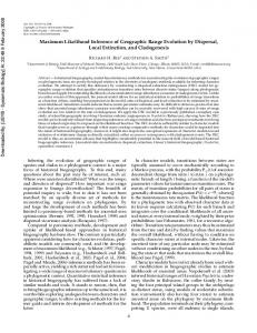
Figure 1: Evolution of state dynamics of a multiresolution process on a lattice. where the subscript i in the vector xi(m) is the translation index at the m-th scale. The superscript T denotes block transposition, and the symbol \*" denotes the adjoint of an operator. Hm is a vector version of the \coarsening" operator [2], which can be viewed as a low-pass ltering operation followed by decimation by a factor of two. A(m); C (m) are block matrices, with blocks corresponding to the vectors xi (m). Hence, the state of the process at each scale m and translation index i is a linear transformation of the state components at the coarser level, corrupted by additive Gaussian noise, as depicted in Figure 1. Given a particular wavelet and its corresponding Hm , a process in this class is characterized by
A(m) E fw(i)w(j)g Q(m) C (m) E fv(i)v(j)g R(m)
= = = = = =
diag(: : :; A(m); : : :; A(m); : : :); Q(i)�ij ; diag(: : :; Q(m); : : :; Q(m); : : :); diag(: : :; C(m); : : :; C(m); : : :); R(i)�ij ; diag(: : :; R(m); : : :; R(m); : : :);
where A(m); Q(m); C(m); R(m) are nite-dimensional matrices. Since the state xi(m) is a vector, rather than a scalar, we allow for higher-order models (in scale). This class of processes is very rich: it includes, for example, the 1=f processes [6], and it approximates other well-studied processes [1].
3. PARAMETER ESTIMATION ALGORITHM
In this section, we solve the problem of estimating the free parameters in A(m); Q(m); C(m); R(m) using observations from either multiple scales or a single scale (e.g. the nest). For measurements exclusively at
the nest scale we can view the parameter estimation problem as tting the parameters of a multiscale model to a time-series. The parameter estimation algorithm that we present consists of two basic steps. The scale state-space model is rst transformed into a set of nite-dimensional state-space models using the wavelet transform; then the parameters are estimated using the EM algorithm. As it is shown in [1], the Karhunen-Loeve expansion for the covariance function of the processes that we examine can be achieved using the wavelet transform. In particular, the model described in eq. (1) can be transformed, by taking its projection onto the wavelet functions vkj (m) at scale j and time k, into a collection of nite dimensional state-space models xj;k(m + 1) = A(m + 1)xj;k (m) + wj;k (m + 1) yj;k (m) = C(m)xj;k (m) + vj;k (m + 1) (2) where the transformed quantities above are xj;k (m) wj;k (m) yj;k (m) vj;k (m)
= = = =
(x(m))T vkj (m) (w(m))T vkj (m) (y(m))T vkj (m) (v(m))T vkj (m)
where (x(m))T ; (w(m))T are dx � 2m matrices, (y(m))T ; (v(m))T are dy � 2m , and dx ; dy are the dimensions of the state and observation vectors respectively. The wavelet function vkj (m) is a 2m � 1 vector, de ned as mY ?1 Hi� )G�j �k vkj (m) = ( i=j +1
where �k is an indicator vector with a 1 in the k-th position, Hi is the coarsening and Gi the di�erencing operator. Thus, the parameter estimation problem now becomes equivalent to that of estimating the parameters of a standard dynamical system from multiple \runs" (e.g., sequences of observations). The sequences of observations yj;k (m) for di�erent wavelet functions vkj (m) have the same dynamics, although the lengths of the observations di�er, and are independent of each other: for (j; k) 6= (j 0 ; k0) the driving terms wj;k (m); wj 0;k0 (m0 ) are independent of each other for all m; m0 because of the orthogonality of the wavelet functions. This problem can be solved using classical parameter estimation methods, where the likelihood function is rst expressed in terms of the prediction error with the aid of a time-varying Kalman predictor and then maximized with respect to the parameters using iterative optimization methods. These methods, however, become too complex in the time-varying case or, in our case, \scale" varying (i.e. when the system parameters
are a function of the scale m). In addition, these methods are not applicable when we have observations only at the nest scale. An alternative method for the maximum likelihood identi cation of a stochastic linear system is based on the observation that the computation of the ML estimates would be simple if the state of the system were observable. The EM algorithm provides an approach for estimating parameters for processes having unobserved components, in this case the state vectors, and therefore can be used for ML identi cation of dynamical systems. Since the noise process is assumed to be Gaussian, the EM algorithm simply involves iteratively computing the expected rst- and second-order su�cient statistics of the state and observation vectors given the current parameter estimates. For the dynamical system case, the two steps of the EM algorithm are derived in [4]. The expectation step is based on a variation of the xed-interval Kalman smoother, and is summarized in Table 1. The recursions are applied independently on each \run" (e.g. projection of the original observations onto a particular wavelet function); in Table 1 we have dropped the subscripts characterizing the wavelet function for simplicity. The expected rstand second-order su�cient statistics that are accumulated during the E-step are summarized below, E fx(m)jYg = x^(m; L) E fx(m)x0 (m)jYg = �(m; L) + x^(m; L)^x0(m; L) E fx(m)x0 (m ? 1)jYg = �(m; m ? 1; L) + x^(m; L)^x0 (m ? 1; L) � y(m); if observed; E fy(m)jYg = C (m)E fx(m)jYg; if missing. 8 y(m)y0 (m); >
E fy(m)y0 (m)jYg =
: R(m) + C (m)E fx(m)x0 (m)j
if missing. ( y(m)E fx0 (m)j g; if observed; E fy(m)x0 (m)j g = C (m)E fx(m)x0 (m)j g; if missing,
Y
Y
Y
where Y denotes the collection of observations at all scales, and x0 is the transpose of x. During the maximization step, estimates of the system parameters are obtained from these statistics using multivariate regression methods. As shown in [4], the EM-based estimation method can also be used to estimate the parameters from sequences of \incomplete" observations, which is very convenient for our case: the problem of estimating the parameters of a multiscale system from observations at a single (the nest) scale can be solved by treating the observations at the coarser scales as missing, e.g. the quantity Y above would consist of the nest-scale observations only.
Forward recursions x^(m; m) x^(m + 1; m) e(m) K (m)
�em �(m; m) �(m; m ? 1; m) �(m + 1; m)
= = = = = = = =
x^(m; m ? 1) + K (m)e(m) A(m)^x(m; m) y(m) ? C (m)^x(m; m ? 1) �(m; m ? 1)C 0(m)[�em ]?1 C (m)�(m; m ? 1)C 0 (m) + R(m) �(m; m ? 1) ? K (m)�em K 0 (m) (I ? K (m)C (m))A(m ? 1)�(m ? 1; m ? 1) A(m)�(m; m)A0 (m) + Q(m)
Backward Recursions x^(m ? 1; L) = x^(m ? 1; m ? 1) +B(m)[^x (m; L) ? x^(m; m ? 1)] �(m ? 1; L) = �(m ? 1; m ? 1) +B(m)[�(m; L) ? �(m; m ? 1)]B0 (m) B(m) = �(m ? 1; m ? 1)A0 (m ? 1)�(m; m ? 1)?1 �(m; m ? 1; L) = �(m; m ? 1; m) + [�(m; L) ? �(m; m)] �?1 (m; m)�(m; m ? 1; m)
Table 1: Summary of E-step recursions
4. NUMERICAL EXAMPLES
In this section we provide numerical examples of applying our identi cation algorithm to synthesized data. We synthesize data using our multiscale state-space models and apply our algorithm to this data to demonstrate the accuracy of the algorithm. In all the examples in this paper we used the Haar wavelet in eq. (1). We apply our algorithm to data given at multiple scales as well as to data at a single (the nest) scale.
Convergence
In Table 2, we present a one-dimensional (dx = dy = 1) example that demonstrates the convergence of the algorithm. In this example the system parameters were A(m) = 0:9; Q(m) = 1; R(m) = 0:1 for all m. The observation matrix was constrained to be C(m) = 1, and the observations from all scales were used for identi cation. We used 11 scales, with L = 0 the coarsest and M = 10 the nest.
E�ects of Data Length
In Table 3 we compare the estimation results for di�erent numbers of scales and di�erent numbers of observations at the nest scale. The estimation error decreases when the number of scales and the number of observations at the nest scale increase from 9 and 256 to 11 and 1024 respectively.
Multiscale Data Versus Single Scale Data
In this subsection we demonstrate that our algorithm can also be used to identify systems that evolve in scale
and for which only observations of the nest scale are available. In particular, we synthesized data for a system with a 2-D state, with the state-transition matrix �
1:0 A(m) = ?0:0 0:7 0:5
�
and unit driving and measurement noise variances. The �observation� matrix was constrained to be C(m) = 0:0 1:0 . The number of scales was again 11 in this example, with scale M = 10 the nest. In Table 4 we summarize the estimation results using observations from all scales, two scales (5 and 10) and only the nest one. We can see that the estimation error increases when data from fewer scales are used. Nevertheless, even in the single-scale case we can get an estimate of the eigenvalues of the state transition matrix, although the observed sequences consist of a single point.
REFERENCES
[1] K. C. Chou, S. Golden and A. S. Willsky, \Modeling and Estimation of Multiscale Stochastic Processes," in IEEE Int. Conf. Acoust., Speech, Signal Processing, pp. 1709{1712, Toronto, Canada, May 1991 (journal paper version accepted for publication in Signal Processing). [2] I.Daubechies, \Orthonormal Bases of Compactly Supported Wavelets," in Commun. Pure Appl. Math.,, Vol. 41, pp. 909{996, November 1988. [3] A. P. Dempster, N. M. Laird and D. B. Rubin, \Maximum Likelihood Estimation from Incomplete Data," Journal of the Royal Statistical Society (B), Vol. 39, No. 1, pp. 1{38, 1977. [4] V. Digalakis, J. R. Rohlicek and M. Ostendorf, \ML Estimation of a Stochastic Linear System with the EM Algorithm and its Application to Speech Recognition," accepted for publication in the IEEE Trans. Signal Processing. A shorter version also appeared in IEEE Int. Conf. Acoust., Speech, Signal Processing, pp. 289{292, Toronto, Canada, May 1991. [5] S. G. Mallat, \A Theory for Multiresolution Signal Decomposition: the Wavelet Representation," in IEEE Trans. Pattern Anal. Mach. Intel., Vol. PAMI-11(7), pp. 674{693, July 1989. [6] G. W. Wornell, \A Karhunen-Loeve-like Expansion for 1=f Processes via Wavelets," in IEEE Trans. Information Theory, Vol. 36, No. 4, pp. 859{861, July 1990.
Actual Iter. 1 Iter. 5 Iter. 10 Iter. 20 Iter. 50 Iter.100 Iter.200
A
Q
R
0.9 0.726 0.981 0.992 0.962 0.925 0.905 0.890
1.0 1.066 0.699 0.718 0.804 0.909 0.969 1.012
0.1 0.918 0.460 0.364 0.287 0.197 0.149 0.114
Table 2: Estimation of A, Q and R as a function of the number of iterations.
A Actual 9x256 11x1024
Q
R
0.9 1.0 0.1 0.937 1.215 0.074 0.890 1.012 0.114
Table 3: Estimation of A, Q and R for di�erent lattice sizes.
Eigenvalues Actual All scales Scales 5, 10 Scale 10
Q
R
0:250 � j0:798 1.0 1.0 0:279 � j0:820 0.929 1.203 0:299 � j0:782 1.128 0.943 0:334 � j0:661 1.077 1.009
Table 4: Estimation of system parameters from subsets of scales.