Maximum Likelihood Sound Source Localization and ... - CiteSeerX

JOURNAL OF LATEX CLASS FILES, VOL. 6, NO. 1, JANUARY 2007

1

Maximum Likelihood Sound Source Localization and Beamforming for Directional Microphone Arrays in Distributed Meetings Cha Zhang, Member, IEEE, Dinei Florêncio, Senior Member, IEEE, Demba E. Ba and Zhengyou Zhang, Fellow, IEEE,

Abstract—In distributed meeting applications, microphone arrays have been widely used to capture superior speech sound and perform speaker localization through sound source localization (SSL) and beamforming. This paper presents a unified maximum likelihood framework of these two techniques, and demonstrates how such a framework can be adapted to create efficient SSL and beamforming algorithms for reverberant rooms and unknown directional patterns of microphones. The proposed method is closely related to steered response power-based algorithms, which are known to work extremely well in real-world environments. We demonstrate the effectiveness of the proposed method on challenging synthetic and real-world datasets, including over 6 hours of recorded meetings.

(a)

Index Terms—Microphone array, sound source localization, beamforming, directional mics

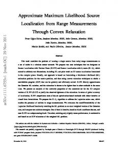
I. I NTRODUCTION Electronically steerable arrays of microphones have recently found a variety of new applications, such as human-computer interaction [1], [2] and intelligent rooms [3]–[5]. A microphone array based system has a number of advantages over a single microphone system. For instance, it may be electronically aimed to capture an audio signal from a desired source location and simultaneously attenuate environmental noises. It can also be used to localize an active speaker nearby, allowing computer controlled devices to provide a nice speaker location aware user interface. To give a more concrete example, a distributed meeting device called RoundTable [6] is shown in Figure 1(a). It has a six-element circular microphone array at the base, and five video cameras at the top. The captured videos are stitched into a 360 degree panorama, which gives a global view of the meeting room (but at low resolution due to bandwidth constraints). The microphone array is there not only to capture superior sounds, but also to detect the sound source location and generate a high-resolution video of the speaker for a better viewing experience. The device enables remote group members to hear and view meetings live online. In addition, the meetings can be recorded and archived, allowing people to browse them afterwards. The key technologies involved in microphone arrays are sound source localization (SSL) and beamforming, both havCha Zhang, Dinei Florêncio and Zhengyou Zhang are with Microsoft Research, Redmond, WA, 98052 USA email: {chazhang,dinei,zhang}@microsoft.com. Demba E. Ba is with Dept. of Electrical Eng. and Computer Science, Massachusetts Institute of Technology, Cambridge, MA 02139 USA Manuscript received Feb. 2007; revised June 2007.

(b)

Fig. 1. RoundTable and its captured images. (a) The RoundTable device. (b) Two images captured by the device.

ing been active research topics since the 1970’s [7]–[9]. A large number of SSL and beamforming algorithms have been proposed in the literature, with varying degrees of accuracy and computational complexity. In this paper, we limit our attention to algorithms that are applicable in distributed meeting scenarios, such as the set of microphones in the RoundTable device. These microphone arrays often bear the following set of characteristics: •

•

•

•

•

The number of microphones in a single device is often limited, e.g., four, six or eight. Linear arrays and circular arrays are the most popular ones. Both omnidirectional and directional microphones are popular. In the case of the circular array in RoundTable, directional microphones are preferred due to their superior sound capture capability. Microphones in distributed meeting devices tend to be spaced at distances around 10 centimeters. The difference in source energy at the microphone locations is not significant. Meeting rooms can receive special sound-treatment, or not. In the latter case, reverberation could be significant due to common reflective objects such as whiteboards or displays. Many distributed meeting devices need to function prop-


erly without a linked computer. The available computational resources are thus very limited. Given these characteristics, the choices for SSL and beamforming algorithms are very limited. For instance, SSL algorithms that rely on sensing the difference in source energy among different microphones cannot be applied due to the close distance between microphones. If the distributed meeting device is to be mass produced, measuring the microphones’ directional response patterns for each device would be extremely difficult if not impossible, hence the algorithm must adapt to microphones with unknown gains. The algorithm also has to be very robust to reverberation, which could change significantly from room to room in the real world. Lastly, any algorithm used in such devices has to be computationally very efficient. In this paper, we present a maximum likelihood (ML) framework for microphone array sound source localization and beamforming. While this is not the first time ML estimation is applied for SSL or beamforming [10]–[13], this paper builds a much stronger connection between the proposed ML-based SSL (ML-SSL) and the popular steered response power (SRP) based algorithms, which are known to work extremely well in practical environments [3], [14], [15] and have very low computational cost. We demonstrate within the ML framework how reverberation can be dealt with by introducing an additional term during noise modeling, and how the unknown directional patterns of microphone gains can be compensated for from the received signal and the noise model. The result is a new and efficient SSL algorithm that can be applied to various kinds of microphone arrays, even for challenging cases such as circular directional arrays with unknown directional patterns (e.g., the array in RoundTable). The effectiveness of the proposed method is shown on both synthetic and real-world data. The synthetic data allows a more precise study of the influence of noise level and reverberation in the algorithm performance. The extensive real-world data corroborates the improvement in relevant scenarios. This data consists of 99 sequences, totaling over 6 hours of meetings, recorded in over a dozen different meeting rooms. Additionally, our ML derivation demonstrates that the traditional minimum variance distortionless response (MVDR) beamforming technique is equivalent to the ML-SSL. In other words, we show that the result of ML-SSL is the same as if one uses multiple MVDR beamformers to perform beamforming along multiple hypothesis directions and picks the output direction which results in the highest signal to noise ratio. The technique proposed above to handle unknown directional patterns of microphone gains can thus be extended to MVDR. We call the revised algorithm enhanced MVDR (eMVDR), and show that it outperforms the traditional method for circular directional microphone arrays. The rest of the paper is organized as follows. We review a number of related SSL and beamforming approaches in Section II. The ML framework is derived in Section III. Using the proposed framework, we derive an efficient SSL algorithm and compare it with various existing approaches in Section IV. eMVDR is discussed in Section V. Experimental results and conclusions are given in Section VI and VII, respectively.

2

II. R EVIEW OF E XISTING A PPROACHES We now review some existing SSL and beamforming approaches that are closely related to the proposed algorithm. A. SSL For broadband acoustic source localization applications, such as teleconferencing, a number of SSL techniques are popular, including those based on steered-beamformer (SB), high-resolution spectral estimation, time delay of arrival (TDOA) [9], and learning [16]. Among them, the TDOA-based approaches have received extensive investigation [3], [9], [17]– [20]. Consider an array of P microphones. Given a source signal s(t), the signals received at these microphones can be modeled as [7], [9], [18], [20]: xi (t) = αi s(t − τi ) + ni (t),

(1)

where i = 1, · · · , P is the index of the microphones; τi is the time of propagation from the source location to the ith microphone location; αi is a gain factor (including the effects of the propagation energy decay, the gain of the corresponding microphone, the directionality of the source and the microphone, etc.), and ni (t) is the noise sensed by the ith microphone. Depending on the application, this noise term could include a room reverberation term to increase the robustness of the derived algorithm [15], [19], which will be discussed in detail in Section IV. It is usually more efficient to work in the frequency domain, where we can rewrite the above model as: Xi (ω) = αi (ω)S(ω)e−jωτi + Ni (ω).

(2)

We can rewrite the above equation into a vector form as: X(ω) = S(ω)G(ω) + N(ω),

(3)

where X(ω) G(ω) N(ω)

= = =

[X1 (ω), · · · , XP (ω)]T , [α1 (ω)e−jωτ1 , · · · , αP (ω)e−jωτP ]T , [N1 (ω), · · · , NP (ω)]T .

Among the variables, X(ω) represents the received signals, hence it is known. G(ω) can be estimated or hypothesized during the computation process, which will be detailed later. The most straightforward SSL algorithm, is to take a pair of microphones, and estimate the difference in time of arrival by finding the peak of the cross-correlation (the direction of arrival is obtained by a geometric transformation from the time of arrival difference and the distance of the mics). For instance, the correlation between the signals received at microphone i and k is: Z Rik (τ ) = xi (t)xk (t − τ )dt. (4) The τ that maximizes the above correlation is the estimated time delay between the two signals. In practice, the above cross-correlation function can be computed more efficiently in the frequency domain as: Z Rik (τ ) = Xi (ω)Xk∗ (ω)ejωτ dω, (5)


3

where ∗ represents complex conjugate. If we substitute (2) into (5), and assuming noise and source signal are independent, the τ that maximizes the above correlation is τi − τk , which is the actual delay between the two microphones. To find the τ that maximizes (5), one simple and extendable solution is through hypothesis testing. That is, hypothesize the source at certain location s, which can be used to compute τi and τk . The hypothesis that achieves the highest crosscorrelation is the resultant source location. When more than two microphones are considered, we sum over all possible pairs of microphones (including self pairs) and have: R(s)

= = =

P X P X

i=1 k=1 Z hX P

Z =

Rik (τi − τk )

i=1 k=1 P X P Z X

i=1 P ¯X

¯ ¯

Xi (ω)Xk∗ (ω)ejω(τi −τk ) dω

Xi (ω)ejωτi

P ih X

Xk (ω)ejωτk

(6) i∗

dω

k=1

¯2 ¯ Xi (ω)ejωτi ¯ dω.

(7)

i=1

Again we can solve the maximization problem through hypothesis testing on potential source locations s. Equation (7) is also known as the steered response power (SRP) of the microphone array. To address the reverberation and noise that may affect SSL accuracy, researchers found that adding a weighting function in front of the correlation can greatly help. Equation (6) is thus rewritten as: P X P Z X R(s) = Ψik (ω)Xi (ω)Xk∗ (ω)ejω(τi −τk ) dω, (8) i=1 k=1

where Ψik (ω) is a weighting function. A number of weighting functions have been investigated in the literature [7]. Among them, the heuristic-based PHAT weighting is defined as: 1 1 Ψik (ω) = = . (9) |Xi (ω)Xk∗ (ω)| |Xi (ω)||Xk (ω)| PHAT has been found to perform very well under realistic acoustic conditions [3], [15]. Inserting (9) into (8), we get: Z ¯X P Xi (ω)ejωτi ¯¯2 ¯ R(s) = ¯ (10) ¯ dω. |Xi (ω)| i=1 This algorithm is called SRP-PHAT [14]. Note that SRP-PHAT is very efficient to compute, because the time complexity drops from P 2 in (8) to P . A more theoretically-sound weighting function is the maximum likelihood (ML) formulation derived by Brandstein et al [9] under an assumption of high signal-to-noise ratio and no reverberation. The weighting function of a microphone pair is defined as: |Xi (ω)||Xj (ω)| . (11) Ψij (ω) = |Ni (ω)|2 |Xj (ω)|2 + |Nj (ω)|2 |Xi (ω)|2 Equation (11) can be inserted into (8) to obtain an ML-based algorithm. This algorithm is known to be robust to noises,

but its performance in real-world applications is relatively poor, because reverberation is not modeled in its derivation. In [15], Rui and Florêncio developed an improved version by considering the reverberation explicitly in the noise term. In a manner similar to the formulation in [3], the reverberation is treated in [15] as another type of noise, i.e.: |Nic (ω)|2 = γ|Xi (ω)|2 + (1 − γ)|Ni (ω)|2 ,

(12)

where Nic (ω) is now the combined noise or total noise. The first term on the right side of (12) is based on the assumption that the reverberation noise energy is proportional to the source signal energy. Equation (12) is then substituted into (11) (replacing Ni (ω) with Nic (ω)) to obtain the new weighting function. Follow-up work [21] proposed a further approximation to yield: Z ¯X P ¯2 Xi (ω)ejωτi ¯ ¯ R(s) = ¯ (13) ¯ dω, γ|X (ω)| + (1 − γ)|N (ω)| i i i=1 whose computational efficiency is close to that of SRP-PHAT. Note, however, that algorithms derived from (11) are not true ML algorithms for multiple microphones. This is because the optimal weight in (11) was derived only for two microphones. When more than 2 microphones are used, the adoption of (8) assumes that pairs of microphones are independent and hence that their likelihoods can be multiplied together, which is questionable. In this paper, a true ML algorithm will be developed for the case of multiple microphones. We will show the connection between the new algorithm and the existing algorithms in Section IV. B. Beamforming Beamforming refers to the technique that aims at improving captured sound quality by exploiting the diversity in the received signals of the microphone array. Depending on the location of the source and the interference, beamforming sets different gains to each mic to achieve its goal of noise suppression. Early designs were generally “fixed” beamformers (e.g., delay-and-sum), adapting only to the location of the desired source. More recent designs are based on “null-steering”, and adapt to characteristics of the interference as well. The minimum variance distortionless response (MVDR) beamformer and its associated adaptive algorithm, the generalized sidelobe canceler (GSC) [22], [23], are probably the most widely studied and used beamforming algorithms, and form the basis of some commercially available arrays [24]. Assuming the direction of arrival (DOA) of the desired signal is known, we would like to determine a set of weights w(ω), such that wH (ω)X(ω) is a good estimate of S(ω). Note X(ω) and S(ω) were defined in (3); superscript H represents Hermitian transpose. The beamformer that results from minimizing the variance of the noise component of w(ω)H X(ω), subject to a constraint of unity gain in the DOA direction, is known as the MVDR beamformer. The corresponding weight vector w(ω) is the solution to the following optimization problem: min w(ω)H Q(ω)w(ω), s.t. w(ω)H G(ω) = 1,

w(ω)

(14)


4

where Q(ω) is the covariance matrix of the noise component: H

Q(ω) = E[N(ω)N (ω)].

(15)

In general, Q(ω) is estimated from the data and therefore inherently contains information about the location of the sources of interference, as well as the effect of the sensors on those sources. The optimization problem in (14) has an elegant closedform solution [25] given by: Q(ω)−1 G(ω) w(ω) = . G(ω)H Q(ω)−1 G(ω)

hypothesis testing. That is, hypotheses are made about the source location, which gives G(ω). The likelihood is then evaluated. The hypothesis that results in the highest likelihood is determined to be the output of the SSL algorithm. Instead of maximizing the likelihood in (18), we minimize the following negative log-likelihood: J

=

(16)

Note that the denominator of (16) is merely a normalization factor which enforces the unity gain constraint in the look direction. In practice, the DOA of the desired signal is not known exactly, which significantly degrades the performance of the MVDR beamformer [26]. Significant effort has gone into a class of algorithms known as robust MVDR [25], [27]. As a general rule, these algorithms work by specifying a region instead of a single look direction where the source has near unity gain. Little attention has been paid to the gain term G(ω) in (16), and most existing work assumes that it is either known or that the α(ω) term can be ignored. This works well for linear arrays, where all microphones point in the same direction ( and hence have similar gains across the mics). However, for the circular geometry such as that of RoundTable, this directionality is accentuated: each microphone will have a significantly different direction of arrival in relation to the desired source. In this paper, we will address this issue by estimating the α(ω) term explicitly during the beamforming process.

=

=

− log p(X|S, G, Q) Z £ J(ω) ¤ − log ρω − dω 2 Zω 1 J(ω)dω − Θ. 2 ω

(21)

R Where Θ = ω log ρω dω is a constant. Since we assume the probabilities over the frequencies are independent of each other, we may minimize each J(ω) separately by varying the unknown variable S(ω). Given that Q−1 (ω) is a Hermitian symmetric matrix, Q−1 (ω) = Q−H (ω), if we take the derivative of J(ω) with respect to S(ω), and set it to zero, we have: ∂J(ω) = −G(ω)T Q−T (ω)[X(ω) − S(ω)G(ω)]∗ = 0. (22) ∂S(ω) Therefore, S(ω) =

GH (ω)Q−1 (ω)X(ω) . GH (ω)Q−1 (ω)G(ω)

(23)

Interestingly, Equation (23) is identical to the MVDR filter by (16). This relationship between the MVDR beamformer and the ML estimator was discovered earlier in [11]. Substituting the above S(ω) into (20), we can write: J(ω) = J1 (ω) − J2 (ω),

(24)

where III. T HE M AXIMUM L IKELIHOOD F RAMEWORK To assure a mathematically trackable solution, we assume the noise of the microphones follows a zero-mean, independent between frequencies, joint Gaussian distribution, i.e., n 1 o pω (N(ω)) = ρω exp − [N(ω)]H Q−1 (ω)N(ω) , (17) 2 where ρω is a normalization constant. When the covariance matrix Q(ω) can be calculated/estimated from known signals, the likelihood of the received signals can be written as: Y p(X|S, G, Q) = pω (X(ω)|S(ω), G(ω), Q(ω)), (18) ω

where pω (X(ω)|S(ω), G(ω), Q(ω)) = ρω exp

n −

J(ω) o , 2

(19)

and J(ω) = [X(ω) − S(ω)G(ω)]H Q−1 (ω)[X(ω) − S(ω)G(ω)]. (20) The goal of the proposed framework is thus to maximize the above likelihood, given the observations X(ω), gain matrix G(ω) and noise covariance matrix Q(ω). Note that the gain matrix G(ω) requires information about the location of the source. Hence, the optimization is usually solved through

= XH (ω)Q−1 (ω)X(ω) (25) H −1 H H −1 [G (ω)Q (ω)X(ω)] G (ω)Q (ω)X(ω) J2 (ω) = . GH (ω)Q−1 (ω)G(ω) (26)

J1 (ω)

Note that J1 (ω) is not related to the hypothesized locations during hypothesis testing. Therefore, the ML-based SSL algorithm shall maximize: Z J2 = J2 (ω)dω ω Z [GH (ω)Q−1 (ω)X(ω)]H GH (ω)Q−1 (ω)X(ω) dω. = GH (ω)Q−1 (ω)G(ω) ω (27) Due to (23), we can rewrite J2 as: Z |S(ω)|2 J2 = dω. H −1 (ω)G(ω)]−1 ω [G (ω)Q

(28)

The denominator [GH (ω)Q−1 (ω)G(ω)]−1 can be shown to be the residue noise power after MVDR beamforming [25]. Hence the ML-based SSL algorithm is equivalent to forming multiple MVDR beamformers along multiple hypothesis directions and picking the output direction as that it results in the highest signal-to-noise ratio.


5

IV. A N E FFICIENT SSL A LGORITHM FOR D ISTRIBUTED M EETING A PPLICATIONS The above derived ML framework is very general. For instance, a similar ML SSL framework was presented in [12]. There, the goal was not only to estimate the location of the sound source, but also its directionality. A model similar to (3) was used, but the noise covariance matrix was assumed to be diagonal, Q(ω) = σI, where σ is independent of the microphone index and frequency. This led to a simplified objective function: Z X ¯2 ¯ P ∗ ¯ (29) α (ω)Xi (ω)ejωτi ¯ dω. J2 = ω

i=1

It is not difficult to verify that under these assumptions, Equation (29) can be easily obtained from (27). On the other hand, Equation (27) cannot be directly applied to perform SSL in our current distributed meeting applications. In particular: • The algorithm is too complex. If a full covariance matrix Q(ω) is used, a P × P matrix inversion has to be conducted for each frequency bin, and the associated matrix multiplication (e.g., GH (ω)Q−1 (ω)G(ω)) has to be conducted for each frequency bin and for each hypothesis source location. • Reverberation is not modeled in (27). • For directional microphone arrays, the gain vector G(ω) remains undetermined. In the following, we will revise the noise model so that it can take reverberation into consideration. The Q(ω) matrix will be diagonalized for fast computation. The gain vector will be explicitly estimated from the received signals and the noise model. A. Reverberation The reverberation of the room environment can be modeled as follows: Nr (ω) = S(ω)H(ω), (30) where H(ω) = [H1 (ω), · · · , HP (ω)]T is the room response function. We define the combined total noise as: Nc (ω) = Nr (ω) + N(ω),

(31)

and we assume the combined noise still follows a zero-mean, independent between frequencies, joint Gaussian distribution. The covariance matrix is: Qc (ω) = =

E{Nc (ω)[Nc (ω)]H } E{N(ω)NH (ω)} + |S(ω)|2 E{H(ω)HH (ω)}, (32)

where E{·} stands for expectation. Here we assume the noise and the reverberation are uncorrelated. It should be noted that combining the reverberation term and the noise term to form a combined noise is not the only method to handle reverberation. In [28], Warsitz and Haeb-Umbarch included the room reflection function in the gain term G(ω), and performed beamforming through an

optimization algorithm that can obtain the combined G(ω) directly. Nevertheless, their algorithm only computes the G(ω) to optimize the beamformer’s output SNR, which cannot be directly used to derive the actual sound source location s in (6). The first term in (32) can be directly estimated from the silence periods of the acoustic signals: K 1 X ∗ Nik (ω)Njk (ω), K→∞ K

E(Ni (ω)Nj∗ (ω)) = lim

(33)

k=1

where k is the index of audio frames that are silent. Note that the background noises received at different microphones may be correlated, such as the ones generated by computer fans in the room. If we believe the noises are reasonably independent at different microphones, we can simplify the first term of (32) further as a diagonal matrix: E{N(ω)NH (ω)} = diag(E{|N1 (ω)|2 }, · · · , E{|NP (ω)|2 }). (34) The second term in (32) is related to reverberation. It is generally unknown. For efficient computation, we assume it is also a diagonal matrix: |S(ω)|2 E{H(ω)HH (ω)} ≈ diag(λ1 (ω), · · · , λP (ω)), (35) with the ith diagonal element equal to: λi (ω)

= E{|Hi (ω)|2 |S(ω)|2 } ≈ γ(|Xi (ω)|2 − E{|Ni (ω)|2 }),

(36)

where 0 < γ < 1 is an empirically determined parameter. Equation (36) assumes that the reverberation energy is a fraction of the difference between the total received signal energy and the environmental noise energy; the same assumption was used in [3], [15], and in (12). Note again that (35) is an approximation; reverberation signals received at different microphones are usually correlated, and the matrix should have non-zero off-diagonal elements. Unfortunately, it is generally difficult to estimate the actual reverberation signals or these off-diagonal elements. In addition, a non-diagonal noise covariance matrix would be very expensive to compute in practice. The covariance matrix of the combined noise thus remains a diagonal matrix: Qc (ω) = diag(κ1 (ω), · · · , κP (ω)),

(37)

with the ith diagonal element as: κi (ω)

= λi (ω) + E{|Ni (ω)|2 } = γ|Xi (ω)|2 + (1 − γ)E{|Ni (ω)|2 }.

(38)

(27) can thus be written as: Z J2 = ω

PP i=1

P ¯2 ¯X αi∗ (ω) ¯ jωτi ¯ X (ω)e ¯ dω. ¯ i 2 |αi (ω)| κ (ω) i=1 i

1

κi (ω)

(39)


6

Ignore frequency Dependent weighting

B. Estimating the Gain Factors The gain factor αi (ω) can be accurately measured in some applications. For applications where it is unknown, we may assume it is a positive real number and estimate it as follows: 2

|αi (ω)| |S(ω)|

2

2

≈ |Xi (ω)| − κi (ω) = (1 − γ)(|Xi (ω)|2 − E{|Ni (ω)|2 }), (40)

where both sides represent the power of the signal received at microphone i without the combined noise (noise and reverberation). Therefore, p (1 − γ)(|Xi (ω)|2 − E{|Ni (ω)|2 }) . (41) αi (ω) = |S(ω)|

ML-SSL (this paper) (42) Zero noise

Consider reverberation 2 Mic ML- as part of noise SRP-RUI SSL [9] in [21] (11) (13)

Zero noise

SRP-PHAT in [14] (10)

Diagonal noise covariance matrix ML-SSL in [12] (29)

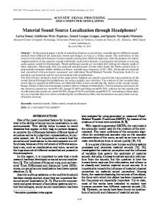
Fig. 2. The relationship graph of the SSL algorithms mentioned in this paper.

by (44). Hence, the previous ML algorithm is conceptually similar to the proposed algorithm. On the other hand, the proposed ML-SSL algorithm differs from the previous method by the presence of the additional frequency-dependent weighting Inserting (41) into (39), we get: ¯2 (denominator in (45)). Furthermore, it has a more rigorous ¯ p 1 jωτi ¯ Z ¯¯ PP 2 2 |Xi (ω)| − E{|Ni (ω)| }Xi (ω)e ¯ derivation, which demonstrates that it is a true ML algorithm i=1 κi (ω) for multiple microphones. J2 = dω. PP 1 2 2 ω To summarize, Fig. 2 shows a relationship graph of the SSL i=1 κi (ω) (|Xi (ω)| − E{|Ni (ω)| }) (42) algorithms mentioned in this paper. Note we use SRP-RUI to The computational cost of the above SSL algorithm is represent the algorithm proposed in [21] (13). The annotations slightly higher than that of SRP-PHAT, but still manageable. on the links between algorithms indicate the conditions to In Section VI, we will demonstrate the superior performance simplify or convert one algorithm to the other. Note the of (42) under various noisy conditions. proposed ML-SSL algorithm is the only one in this graph that is optimal in ML sense for multiple microphones. C. Discussion V. E NHANCED MVDR B EAMFORMING ( E MVDR) The ML-SSL algorithm proposed in (42) is closely related As presented in Section III, the MVDR algorithm, although to existing SRP SSL algorithms in the literature. For instance, when the signal-to-noise ratio (SNR) is very high, we have derived from a very different perspective, is indeed identical |Xi (ω)|2 À E{|Ni (ω)|2 }. Subsequently, κi (ω) = γ|Xi (ω)|2 , to an intermediate step (23) during the derivation of the MLSSL algorithm. Recent MVDR research has mostly focused Equation (42) thus becomes: on how to make MVDR robust to source location errors ¯P ¯2 |Xi (ω)| jωτi ¯ Z ¯¯ P (such errors are usually caused by SSL). In this section, we X (ω)e ¯ 2 i i=1 γ|Xi (ω)| J2 = dω propose an eMVDR approach that tries to address the problem PP |Xi (ω)|2 ω i=1 γ|Xi (ω)|2 of unknown directional patterns of microphones. It should Z ¯X P be noted that existing robust MVDR algorithms can be still jωτi ¯2 1 Xi (ω)e ¯ ¯ = (43) applied on top of our method to further improve performance. ¯ dω ¯ γP |Xi (ω)| i=1 Unlike in SSL, where reverberation can cause errors in which is equivalent to SRP-PHAT (10). Note that since the the output source location, reverberation in beamforming is reverberation parameter γ is a constant factor of J2 , it does usually less of a concern in distributed meetings, because not affect the optimality of SRP-PHAT as long as the noise is the reflected signal can still contain intelligible information. Therefore, in the following discussion, we ignore the reververy low. The connection between the proposed ML-SSL algorithm beration term introduced during SSL (30), and use a noise and the ML algorithm in (11) is not straightforward. Recall covariance matrix directly estimated from the silence period that in their original derivation, Brandstein et al. [9] estimated of the meeting the variance of the phase for a particular frequency as: Q(ω) = E{N(ω)NH (ω)}. (46) V ar[θi (ω)] =

E{|Ni (ω)|2 } . |Xi (ω)|2

(44)

If we ignore reverberation by setting γ = 0, and assume noise is relatively small compared with the signal (the same assumptions were made in [9]), then (42) can be written as: ¯2 ¯ ¯ eθi (ω) ejωτi Z ¯¯ PP i=1 E{|Ni (ω)|2 }/|Xi (ω)|2 ¯ dω. (45) J2 = PP 2 2 ω i=1 |Xi (ω)| /E{|Ni (ω)| } Therefore, the phase term of each microphone eθi (ω) ejωτi is indeed weighted by the inverse of the phase variance, as given

We start our discussion with (23) and (41). From (41), it can be seen that αi (ω) can be estimated from the received signal and the noise model, though it is also related to the actual source energy. Fortunately, in MVDR it is the relative gains among the sensors that really matter in terms of beam shaping. Therefore, we define: α ˆ i (ω)

= =

αi (ω) j=1,...,P αj (ω) p (|Xi (ω)|2 − |Ni (ω)|2 ) p P (|Xi (ω)|2 − |Ni (ω)|2 ) j=1,...,P P

(47) (48)


7

7

3 Ceiling fan 3.5

6

1.5 3.5 6-mic array 1.5 Fig. 3.

Speaker

θ Computer

Top-down view of the virtual room for synthetic experiments.

A new gain vector: ˆ G(ω) = [ˆ α1 (ω)e−jωτ1 , · · · , α ˆ P (ω)e−jωτP ]T

(49)

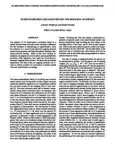
is then inserted in (23) to perform MVDR. It should be noted that by replacing actual gains with relative gains, we no longer compensate for the frequency response of the microphones. For example, if the microphones’ average gain in a certain frequency is high, this will not be compensated for, and the final output signal will be stronger at that frequency. We believe this is not generally a problem, as most microphones have reasonably flat frequency responses. Furthermore, any equalization method used with a single mic could be similarly applied here, after beamforming. VI. E XPERIMENTAL R ESULTS We now present the results of our SSL and beamforming experiments. We run simulations on both synthetic signals and with extensive natural data. A. SSL We test the performance of the ML-SSL algorithm embodied in (42), on both synthetic and real-world datasets. The two benchmark algorithms we use to compare with the MLSSL method are SRP-PHAT (10) and its improved version from [21] (13). Note that SRP-PHAT is a special case of SRPRUI when γ = 1.0, while SRP-RUI is a special case of the ML-SSL algorithm when αi (ω) ≡ α(ω), i = 1, · · · , P , and the frequency weightings are ignored. 1) Experiments on synthetic data: A virtual room with size 7 × 6 × 2.5 meters is created, as shown in Fig. 3. A circular 6-microphone array is placed near the center of the room, at (3.5, 1.5, 1). The radius of the microphone array is 0.135 m. A speaker is talking at a distance of 1.5 m from the center of the microphone array, at an angle θ. We introduce two noise sources in the scene. A ceiling fan is mounted in the middle of the room, at (3.5, 3, 2.5), and a computer is located in the corner, at (7, 0, 0.5). The wave signals from the speaker, the fan and the computer are all recordings from the real world. The reverberation effect of the room is added to all signals according to the image model [29]. The SSL algorithm performs hypothesis testing at 4◦ intervals in azimuth. The reported results are averaged over 10

speaker locations uniformly distributed around the microphone array (θ = 0, 36◦ , ..., 324◦ ). At each location the signal length is 30 seconds. The analysis window of SSL is 40 ms, overlapping by 20 ms. We sample 100 speech frames from each location and perform SSL on them. Table I reports the average accuracy, in terms of what portion of the SSL estimates (totally 1000 frames) is within 2◦ and 10◦ of the ground truth angle. To assess the impact of reverberation on SSL performance, we synthesize rooms with 100 ms and 500 ms reverberation times, as seen in the upper and lower parts of Table I respectively. It can be observed from Table I that SRP-PHAT usually performs as good as ML-SSL when the input SNR is high (20 dB or above), but its performance drops significantly when the SNR becomes low. In most indoor (e.g., offices and meeting rooms) environments, the signal to noise ratio is above 15 dB, which explains SRP-PHAT’s satisfactory performance in practice. SRP-RUI is a very decent and practical SSL algorithm too. In low reverberation environment (top table), SRP-RUI has slightly worse performance than ML-SSL, and both algorithms significantly outperform SRP-PHAT in noisy cases. In high reverberation environment (bottom table), all three algorithms have a significant performance drop. MLSSL still outperforms both SRP-PHAT and SRP-RUI, though by a small margin. For the ML-SSL algorithm, the tunable parameter γ does seem to impact the final performance. This is particularly true when the reverberation is low. For instance, in the top table, when the reverberation is low (100 ms), when the input SNR is 0 dB, choosing γ = 0.1 results in a much better performance than γ = 0.5. This gap is however not significant when reverberation is high (bottom table, 500 ms). Therefore, for practical applications, using a fixed γ ranging from 0.1 to 0.3 can usually result in satisfactory performance. 2) Experiments on real-world data: We next test the MLSSL algorithm on 99 real-world meetings captured by the RoundTable device (Fig. 1). SSL is used in RoundTable to determine for which speaker the high-resolution video is to be provided. One difficulty of SSL for the RoundTable device is that directional microphones are used to capture better audio. For microphones pointing away from the speaker, the estimated phase may be unreliable. In [21], the authors attempt to address the issue by selecting a subset of the microphones for SSL. In this paper, we use all the microphones, since MLbased SSL weights microphones differently based on their SNR automatically. We will compare our results with [21]. The meetings are 4 minutes long each, captured in about 50 different meeting rooms in order to test the robustness of the SSL algorithms in different environments. The noise levels of the rooms and the distances from the speakers to the devices vary significantly, causing the input SNR to range from 5 dB to 25 dB. The speaker locations of 6706 audio frames are labeled manually based on the corresponding face locations in the panoramic image. We report the results on the percentage of frames that are within 6◦ and 14◦ of the ground truth azimuth angle. This is slightly relaxed from the synthetic experiment but good enough for detecting speaker orientation in RoundTable.


8

TABLE I E XPERIMENTAL RESULTS OF SSL ACCURACY ON THE SYNTHETIC DATASET. C ELLS WITH BOLD FONTS INDICATE BEST PERFORMANCE IN THE GROUP. Reverberation = 100 ms = 0.1 Input SNR 25 dB

SRP-RUI

SRP-PHAT

= 0.3 ML-SSL

= 0.5

SRP-RUI

ML-SSL

SRP-RUI

ML-SSL