arrayed in free space, where three or more microphones are essential to localize ..... through a microphone amplifier (AT-MA2; audio-technica). C. Experimental ...
Sound Source Localization by Asymmetrically Arrayed 2ch Microphones on a Sphere Nobutaka Ono∗, Soichiro Fukamachi∗ , Takuya Nishimoto ∗ and Shigeki Sagayama∗ ∗
Graduate School of Information Science and Technology, The University of Tokyo 7-3-1 Hongo Bunkyo-ku, Tokyo, 113-8656 Email: {onono, s-fukamachi, nishi, sagayama}@hil.t.u-tokyo.ac.jp
Abstract— In this paper, we propose a novel system to localize a sound source in any 2D directions using only two microphones. In our system, the two microphones are asymmetrically placed on a sphere, thus, 1) the diffraction by the sphere and the asymmetrical arrangement of the microphones yield the localization cue including the front-back judgment, and 2) unlike the dummy head system, no previous measurements are necessary due to the analytical representation of the sphere diffraction. To deal with reverberation or ambient noises, we consider the maximum likelihood estimation of the direction of arrival with a diffused noise model on a sphere. We present a real system that we built through the investigation of the optimal microphone arrangement for speech, and give experimental results in real environment.
sound signal
。
0
Left microphone
Right microphone
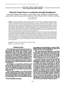
Sphere Fig. 1.
Arrangement of the microphones
I. I NTRODUCTION Localization of sound source is very useful in various acoustic applications such as target tracking, environment monitoring, speaker indexing, and so on. Most of man-made systems are omni-directional pressure-sensitive microphones arrayed in free space, where three or more microphones are essential to localize the 2D direction since a pair of microphones placed in free space has an intrinsic axial symmetry, which brings a front-back ambiguity to the 2D localization. On the other hand, many animals including human have the capability of localizing a sound source from any directions with only two ears [1]. The key is to exploit the frequency characteristic of reflection or diffraction by the pinna or the head. By mimicking the auditory systems, several previous works aim at realizing such abilities as monaural sound source localization [2], [3], [4], DOA estimation of elevation and azimuth using asymmetric reflectors like the ones found in barn owls [5], or human-like localization based on a dummy head system [7], [8]. Especially, the development of sound source localization by 2ch array should enrich PC applications since it can be easily installed on a PC through the standard audio input. It would also facilitate the sound source separation based on a stereo signal [9], [10]. In this paper, inspired from the human auditory mechanism, we propose a novel system to localize a sound source in any 2D directions using only two microphones. In our system, two microphones are asymmetrically arrayed on a sphere, where, instead of the pinna, the diffraction by the sphere and the asymmetrical arrangements of the microphones yield the localization cue including the front-back judgment. Unlike the dummy head, our system doesn’t require consuming HRTF measurements due to the analytical representation of the
diffraction by a sphere. A pilot work has been done by Handzel et al., where they examined through numerical simulations the asymmetric arrangement of two microphones on a sphere and a localization algorithm based on the metric of the interaural level and phase difference [11]. In this paper, to deal with speech sources and real environment including reverberation or ambient noises, we consider the maximum likelihood estimation of the direction of arrival with a diffused noise model on a sphere. Through the investigation of the optimal microphone arrangement for speech, we built a prototype system using a wooden ball with a 30mm radius. We describe the system and give experimental results obtained with it in real environment. II. I NVESTIGATION OF L OCALIZATION P OSSIBILITIES Suppose that two microphones are placed at angles of ±φ on a sphere shown in Fig. 1. When a plane wave arrives from a direction θ, the observed signals M (ω) = (ML (ω), MR (ω))T can be written as M (ω) = S(ω)H (ω, θ) + N (ω),
(1)
where S(ω) is the arriving source signal and N (ω) the observation noise. The frequency characteristics H(ω, θ) depending on the direction of arrival can be written H (ω, θ)
T
=
(HL(ω, θ) HR (ω, θ))
=
(D(ω, θ − φ) D(ω, θ + φ)) .
T
(2)
D in eq. (2) is called the diffraction coefficient, which can be expressed analytically as [12] D(ω, ψ)
=
∞ 1 � j (n+1) (2n + 1)Pn (cos ψ) , ka n=0 ka h(2) (ka) − nh(2) n (ka) n+1
(3)
ITF (φ=90, 1kHz)
ITF (φ=90, 2kHz) 4
4
2
2
2
−2
−4 −4
−2
0 Re
2
−4 −4
4
0
Im
0
Im
−2 −2
0 Re
2
4
−4 −4
ITF (φ=50, 2kHz)
ITF (φ=50, 1kHz)
4
2
2
2
0
0
0
Im
4
−2
−2
−4 −4
−4 −4
−2
0 Re
2
4
−2
0 Re
2
4
ITF (φ=50, 3kHz)
4
Im
Im
0 −2
Im
ITF (φ=90, 3kHz)
4
−2 −2
0 Re
2
4
−4 −4
−2
0 Re
2
4
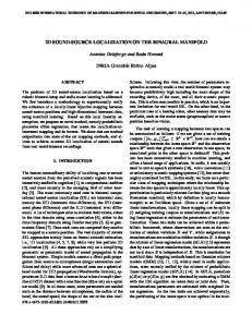
Fig. 3. Loci of ITF for 360 ◦ sound direction in the complex plane for the symmetric arrangement (φ = 90◦ ) (upper) and an asymmetric arrangement (φ = 50◦ ) (lower)
Fig. 2. Interchannel intensity ratio in [dB] (upper) and phase difference in [rad] (lower) for an asymmetrical arrangement (φ = 50◦ ) on a sphere of radius 85mm
(2)
where Pn (x) is the Legendre function, hn (x) is the spherical Hankel function of the second kind, a is the radius of the sphere,ψ the direction of arrival, and k = ω/c where c is the sound velocity. Even if N (ω) = 0 in eq. (1), HL(ω, θ),HR (ω, θ) cannot be directly observed due to the unknown source term S(ω). Thus, in sound source localization, the Inter-channel Transfer Function (ITF) defined by their ratio as ITF(ω, θ) =
HL(ω, θ) D(ω, θ − φ) = HR (ω, θ) D(ω, θ + φ)
(4)
is the significant quantity, which is theoretically independent from S(ω). The pair of interchannel intensity and phase differences, which is often used as a cue of localization in a 2ch array, is equivalent to the ITF. For a localization without ambiguity, a one-to-one correspondence between the ITF and the source directions is necessary. First, we show in Fig. 2 the amplitude and the phase of the ITF for a sphere of radius 85mm and an arrangement corresponding to φ = 50◦ . Despite the absence of pinnalike structures there, we can see that the significant amplitude difference between both channels is introduced only by the diffraction of the sphere. To explore the relationship between the ITF and the source direction, we show several loci of the ITF in the complex plane for the symmetric arrangement (φ = 90◦) and an asymmetric arrangement (φ = 50◦ ) at 1kHz, 2kHz, and 3kHz in Fig. 3.
In the symmetric case, the loci are curves with two endpoints, which means that the ITF is completely overlapped between the front and back directions and these cannot be distinguished (the two endpoints correspond to θ = 90◦ and θ = 270◦ ). While in the asymmetric case, they depict closed loops with a few cross-points, which means that most directions can be localized. The ambiguity of the directions corresponding to the cross-points will be solved by integration of the localization results over frequencies. Note that all loci have a common cross-point at ITF= 1, which corresponds to θ = 0◦ and θ = 180◦. Our system thus cannot distinguish only these two directions because of the intrinsic left-right symmetry. III. L OCALIZATION A LGORITHM B ASED ON ML E STIMATION AND D IFFUSED S OUND F IELD M ODEL Because actual observations include noise, the ITF obtained from an observation M (ω) does not coincide with the theoretical values shown in Fig. 3. Furthermore, the reliability of each frequency band should be different depending on each SN ratio. One reasonable way to perform localization in such a case is to apply maximum likelihood estimation based on some stochastic model of the observation noise [13]. Assuming that N (ω) follows a complex-valued Gauss distribution with mean 0 and covariance matrix V (ω), the logarithmic likelihood is given by 1 log p(M (ω); S(ω), θ) = − log(2π| det V (ω)|) (5) 2 1 − E(ω)h V (ω)−1 E(ω), 2 E(ω) = M (ω) − S(ω)H(ω, θ). (6) Since the unknown source term S(ω) is present in the expression, we replace it by the ML estimation: SM L (ω) =
H(ω, θ)h V (ω)−1 M (ω) , H(ω, θ)h V (ω)−1 H(ω, θ)
(7)
where ωH is the upper limit frequency of the observation and some terms which do not depend on the observation are omitted for simplicity. In the ML estimation described above, the determination of the shape of V (ω) is important. When the noise powers of the left and right observation are equivalent, the covariance matrix V (ω) can be written � � 1 η(ω) 2 V (ω) = σ (ω) , (9) 1 η(ω)∗ where σ(ω)2 is the noise power and η(ω) represents the noise correlation. In a reverberant or ambient-noisy environment, the correlation is indeed not negligible especially when the microphone distance is small. Under the diffused noise field assumption [14], [15] where plane waves of noise arrive randomly from any spherical direction, we here evaluate the correlation statistically as � 2π� π 1 ηD (ω) = D(ω, ψL (ψ1 , ψ2 )) 4π 0 0 ×D(ω, ψR (ψ1 , ψ2 ))∗ sin ψ1 dψ1 dψ2 , (10) (11) ψL (ψ1 , ψ2 ) = cos−1 (sin ψ1 cos(φ − ψ2 )), (12) ψR (ψ1 , ψ2 ) = cos−1 (sin ψ1 cos(φ + ψ2 )). In the case of 3D free space, D(ω, ψ) = e−jωL sin ψ/c , where L is the distance between the two microphones, analytically yields ηD (ω) = sin(ωL/c)/(ωL/c), that is, a sinc function [14]. In the case of the sphere diffraction, we can calculate it numerically using the analytical representation of D in eq. (3). According to our calculation, it is similar to a sinc function. Actually, the real environment is not a perfect diffuse field. Thus, we set η(ω) = α · ηD (ω), (13) where 0 ≤ α ≤ 1, and determine α experimentally. IV. L OCALIZATION E XPERIMENTS IN R EAL E NVIRONMENTS A. Optimization of the Microphone Arrangement In order to obtain the optimum arrangement, we examined the relationship between the position of the microphones and the localization accuracy through simulation. In this experiment, the radius of the sphere was 30mm, the source signal was speech, and Gaussian white noises with 10dB or 0dB SN ratio (two conditions were used) were added into left and right observation signals. The source direction θ changed from 0◦ to 360◦ . The localization accuracy was evaluated by the ratio of estimations inside ±5◦ from the source direction. The result is shown in Fig. 4.
0.8
accuracy rate
and integrate the log-likelihood over frequencies to obtain the total log-likelihood function as � 1 ωH � LL(θ) = (8) −M (ω)h V (ω)−1 M (ω) 2 0 � |H(ω, θ)h V (ω)−1 M (ω)|2 dω, + H(ω, θ)h V (ω)−1 H(ω, θ)
0.6 0.4 0.2 0 0
20
40
60
80
mic configuration (degree) Fig. 4.
Localization accuracy depending on microphone position
For φ > 70◦ and φ < 30◦, the localization accuracy is low. The reason of the former is the difficulty of the front-back judgment due to the arrangement near symmetry, while that of the latter is the smaller difference between the observation signals. Although the accuracy is almost flat between them, we adopted φ = 46◦ which achieves the best accuracy in this experiment. B. Fabrication of the Real System To build the system, for small-size realization, we used two electret type microphones (AT805F; audio-technica) and a wooden ball with a 30mm radius. Microphone-size holes were carved in the ball at ±46◦ in the equator, and the microphones were fixed there. An internal screw was attached at the south pole position and the ball was fixed to a small tripod. A photograph of the constructed system is shown in Fig. 5. The observed signals are readable from the standard audio input through a microphone amplifier (AT-MA2; audio-technica). C. Experimental Conditions and Results The speech signal generated by a speaker was recorded by the system. The distance between them was kept equal to 1m and angles every 30◦ from 0◦ to 180◦ were chosen as the source direction. In the environment, several ambient noises, from fan or HDD, and reverberation are present. The sampling frequency of the recorded signals was 16kHz. The frame length of STFT was 512 samples (32ms), and a Hamming window was used. In the noise covariance of eq. (9), σ 2 (ω) = C was used as a simple white noise model. As for the noise correlation model, both η(ω) = 0 (independent noise model) and η(ω) = 0.5·ηD (ω) (partially diffused noise model) were examined. For a stable localization, the log-likelihood function eq. (8) was accumulated over 10 frames and the source direction was estimated from the maximum every 10 frames (one estimation per 320ms interval). The estimations from the nearly silent intervals are removed by thresholding. The results using the independent noise model (η(ω) = 0) are shown in Fig. 6. The front and back judgment was rather correctly performed but there are about 20% errors. Furthermore, we can see a tendency of the estimations for
180
estimated direction
150 120 90 60 30 0 0
30
60
90
120 150 180
source direction Fig. 6.
Fig. 5.
Photograph of the constructed system
Localization results using the independent noise model
180
◦
front sources (0 < θ < 90 ) to be biased to the front, and similarly for back sources. A reason for this bias is that the correlated component included in the noise is interpreted as the target signal from the direction to yield the highest correlation, that is, the front (θ = 0◦ ) or the back (θ = 180◦) since the noise model doesn’t include any correlation components. Whereas the results using the partially diffused noise model (η(ω) = 0.5 · ηD (ω)) show that the biased estimations were compensated and the errors of front-back judgment were less than 10%, which means that our approach works well. The localization accuracy could be improved by increasing the number of accumulation frames. Thus, a trade-off between localization accuracy and temporal resolution should be determined in every application. V. C ONCLUSIONS In this paper, we discussed a novel localization system for any 2D directions using two microphones asymmetrically placed on a sphere. Using a ML estimation based on the diffused noise model, we showed that the constructed system is able to localize any 2D direction almost correctly in real environment. 2ch BSS based on this system is an interesting future work which we plan to investigate. R EFERENCES [1] J. Blauert, Spatial Hearing, MIT Press, Cambridge, MA, 1983. [2] J. G. Harris, C. J. Pu, and J. C. Principe, “A monaural cue sound localizer,” in Analog Integrated Circuits and Signal Processing, vol. 23, pp. 163–172. 2000. [3] N. Ono, Y. Zaitsu, T. Nomiyama, A. Kimachi, and S. Ando, ”Biomimicry sound source localization with Fishbone,” Trans. Inst. Electrical Engineers of Japan, vol. 121-E, no. 6, pp. 313–319 ,2001. [4] H. Nakashima ,N. Ohnishi, and T. Mukai, “A learning system for estimating the elevation angle of a sound source by using a feature map of sperctrum,” Trans. IEICE D-II, vol. J87-D-II, no. 11, pp. 2034–2044, 2004. (in Japanese) [5] N. Ono and S. Ando, ”Sound Source Localization Sensor with Mimicking Barn Owls,” Proc. Transducers’01, vol.2, pp.1654-1657, Munich, 2001.
estimated direction
150 ◦
120 90 60 30 0 0
Fig. 7.
30
60 90 120 150 180 source direction
Localization results using the partially diffused noise model
[6] N. Ono, A. Saito, and S. Ando, ”Bio-mimicry Sound Source Localization with Gimbal Diaphragm,” Trans. Inst. Electrical Engineers of Japan, vol. 123-E,no. 3, pp. 92-97 ,2003. [7] R. E. Irie, “Multimodal sensory integration for localization in a humanoid robot,” Proc. the Second IJCAI Workshop on Computational Auditory Scene Analysis (CASA ’97), pp 54–58, 1997. [8] H. Nakashima, Y. Chisaki, T. Usagawa and M. Ebata, “Frequency domain binaural model based on interaural phase and level differences,” Acoust. Science & Technology, vol. 24, no. 4, pp. 172–178, 2003. [9] O. Yilmaz and S. Rickard: “Blind Separation of Speech Mixtures via Time-Frequency Masking,” IEEE Trans. Signal Processing, vol. 52, no. 7, pp 1830-1847, 2004. [10] Y. Izumi, N. Ono, and S. Sagayama, “Sparseness-based 2ch BSS Using the EM Algorithm in Reverberant Environment,” Proc. WASPAA2007, 2007. (submitting) [11] A. A. Handzel and P. S. Krishnaprasad, “Biomimetic Sound-Source Localization,” IEEE Sensors Journal, vol. 2, no. 6, pp. 607–616, Dec. 2002. [12] T. Hayasaka and S. Yoshikawa, Onkyo Shindoron (Theory of Acoustic Vibration), Maruzen, Tokyo, 1974. (in Japanese) [13] M. Brandstein and D. Ward, Microphone Arrays, Springer, 2001. [14] R. K. Cook, R. V. Waterhouse, R. D. Berendt, S. Edelmann and M. C. Thompson, “Measurement of correlation coefficients in reverberant sound fields,” JASA, vol. 27, no. 6, pp. 1072-1077, 1955. [15] I. A. McCowan, H. Bourlard, “Microphone Array Post-Filter Based on Noise Field Coherence,” IEEE Trans. on Speech and Audio Processing, vol. 11, no. 6, pp. 709-716, 2003.