IEEE TRANSACTIONS ON MAGNETICS, VOL. 36, NO. 4, JULY 2000
1645
Maxwell Equations and Finite Element Software Systems: Object-Oriented Coding Needs Well Defined Objects Jari Kangas, Timo Tarhasaari, and Lauri Kettunen
Abstract—In this paper we examine the structure of Maxwell equations in order to find clear signposts how to implement finite element software systems. The aim is to recognize the abstractions involved in Maxwell equations and to exploit concepts of modern programming techniques, such as object-oriented design, to imitate the abstractions in numerical computing. As mathematics is the machinery to model physical phenomena, it is worth to imitate the same machinery in a software system. If a software system is constructed this way, it is partitioned into distinct components whose function is evident. And that is a basis for a software system that is modifiable and understandable, which are the main goals in software design. Index Terms—Finite element methods, object-oriented programming.
I. INTRODUCTION
T
HE quality of a software system to solve numerically Maxwell equations is not only defined by its “external” qualifiers such as efficiency and the ease of use, but by its “internal” properties as well, i.e. how new requirements and ideas can be incorporated into the system. Ideally extending the software should be easy and one should be able to benefit from the exponential growth factor: The same amount of work should multiply the power of the product, not only add to it, if the system is well established and designed. Any experience of practice does, however, suggest that meeting such goals is challenging. In fact, a rather common observation is that after the software reaches a certain critical size, the development team has to increase their amount of efforts for every new extension instead of gaining from the previous work. There are, of course, various reasons for the idealism not working in practice, and the restrictions set by the programming languages are not the least of them. Still, the practical experience does also suggest that the many and various numerical approaches for electromagnetism do have, in fact, a lot in common. Hence the question whether a software system for electromagnetics could be designed that enables to reuse—not only readapt—it for new numerical approaches with reasonable effort.
Manuscript received October 25, 1999. The authors are with the Tampere University of Technology, Laboratory of Electromagnetics, P.O. Box 692, FIN-33101 Tampere, Finland (e-mail:
[email protected]). Publisher Item Identifier S 0018-9464(00)04961-X.
Fig. 1. The structure of Maxwell equations shown with the “Maxwell’s house.”
Reusing and extending software to new applications is a serious problem and not only specific to computational electromagnetics. Therefore software specialists have sought for new programming techniques to overcome the apparent difficulties. Object-oriented design [1] is one of these modern tools (among others, see e.g. [2], [3]) intended for better software architecture. The structure of a software system is most clearly defined by using abstractions. Modularity and abstract data types are the key points in implementing abstractions and object-oriented languages provide the tools needed. This is the motivation to examine the structure of Maxwell equations and the mathematical machinery involved in them.
II. MAXWELL EQUATIONS Maxwell equations involve a strong mathematical structure repeating itself from one level to another, see e.g. [4], [5]. This underlying structure can be illustrated with a so called Maxwell’s house [5], Fig. 1. Maxwell’s house provides us with a good starting point: the frame of the software system should imitate on the discrete level the construction of Maxwell equations. The first step is to recognize the abstractions involved in Maxwell equations. This amounts asking what kind of data is vital for the operators, and what the operators do to that data. In other words, we have to peel out all the excessive layers of data an operator does not need, and then detect the new object (i.e. data-structure) the operator creates. As it is an extensive work to formally define all the data types and operations needed in a finite element system for electromagnetics, in this paper we shall focus only on the main aspects and principles.
0018–9464/00$10.00 © 2000 IEEE
1646
IEEE TRANSACTIONS ON MAGNETICS, VOL. 36, NO. 4, JULY 2000
III. METRIC AND NON-METRIC DATA One of the most important tasks in seeking for the data structures for software systems solving Maxwell equations is to distinguish between the metric and nonmetric (or topological) concepts. In Fig. 1 the vertical arrows of the Maxwell house represent nonmetric information—Maxwell equations, indeed, do not depend on metric—whereas the metric data is included in the horizontal arrows (i.e. in the constitutive laws) connecting the left and right hand sides. As vector analysis is built above metric structures, it is not a language powerful enough to make the distinction between metric and nonmetric data. Thus, more powerful tools, such as differential geometry and algebraic topology (which is a branch of mathematics studying properties of geometrical objects and their continuous mappings into each other) have to be considered. The name “algebraic topology” itself already suggests why it is such a useful tool in this context: The very idea is to use algebraic notions and methods—i.e., those which can easily be transferred into pieces of software—in solving topological problems. Notice that nonmetric data can be expressed with pointers and integers, whereas metric data requires real numbers. As computers do execute integer arithmetics exactly, topological data can be handled without any loss of precision. IV. COMPLEX The Maxwell house reflects the basic structure of Ampère’s, Faraday’s, and Gauss’ laws expressing the integrals of fields over cells as integrals of another fields over the boundaries of the same cells. (Of course, only up to time differentiation, which is why we have the front and back sides of the Maxwell house.) The “pointwise” expressions of the integral forms of Maxwell equations are obtained by applying the generalized Stokes theorem (1) This very structure of Maxwell equations is why the exterior derivative and the boundary operator are so strongly related to Maxwell theory. Furthermore, according to Stokes theorem operators and dual to each other, which would be easier to . see, if instead of (1) one wrote Let us now denote by and the sets on which operis ators and act, respectively. (In more precise terms, is the group the space of differential forms of degree and and with , of -chains.) Equipping operators with and called comtwo new compound objects plexes are formed. A complex is one of the most important objects of algebraic topology, and highly useful in computational electromagnetism. On the discrete level, what is usually called a finite ele, where the , ment mesh is a (cellular) complex are the groups generated by sets of nodes, edges, faces, and volumes. The 1-to-1 counterpart of the (primal) finite element mesh, i.e. the so called dual mesh, is obviously also a complex. If the corresponding groups of dual cells are denoted
Fig. 2. Left: The primal and dual meshes are complexes and in one-to-one correspondence to each other. Right: The spaces of DoFs equipped with matrices d and d representing the exterior derivative and its adjoint on the discrete level, respectively, form complexes which are isomorphic to each other.
by , then these complexes can be illustrated graphically as shown in Fig. 2. On the discrete level fields (i.e., differential forms) correspond with arrays (or vectors) of degrees of freedom (DoFs), , the spaces they span, and we shall denote by , where is the dimension. The arrays of the DoFs associated . Spaces with the cells of the dual mesh span spaces and represent spaces in which the two “sides” of a field and live. For instance, in case of magnetic field spaces are the spaces of fluxes across facets and of magnetomotive forces along (dual) edges, respectively. According to the conand are isomorphic to each other stitutive laws spaces and we shall denote by the operator—the matrix—mapping onto and vice versa. (In other words, the is from the discrete counterpart of the Hodge operator [6], [7]). For inand the array stance, in 3D the array of fluxes belongs to of magnetomotive forces along the edges of the dual mesh . In this case there is a square matrix such that is part of representing the constitutive law on the discrete level. The discrete counterpart of the exterior operator is also a matrix and it is commonly denoted by . (This is a so called , incidence matrix.) Equipping with spaces a complex can be formed. As the adjoint operator of is its transpose , for the dual side DoFs we have another , and these two complexes are isomorphic to complex each other via the -operator, see Fig. 2. Notice, that the metric data of the system is implied by the horizontal arrows of the diagram on right in Fig. 2. All the other arrows in Fig. 2 represent nonmetric relations. V. SEQUENCES AND DECOMPOSITIONS One of the basic properties of operators
and
is that
and (The former is a metric independent counterpart of curl grad 0 and div curl 0, and the latter says “the boundary of a boundary has to always vanish.”) This implies that the codomain has to be a subset of the kernel of (or range) of (of (of , resp.), i.e. cod
ker
and
cod
ker
Those fields which belong to cod( ) are called exact (forms) and those which belong to ker( ) are said to be closed (forms).
KANGAS et al.: MAXWELL EQUATIONS AND FINITE ELEMENT SOFTWARE SYSTEMS
Correspondingly, a set of chains which is a subset of ker( ) is called a cycle, and those chains which are part of cod( ) are bounding cycles. (For instance, a set of edges forming a “loop” is a cycle. If it is also a boundary of some surface, then it is also a bounding cycle.) Let us denote the spaces of closed and and , exact DoF-arrays of degree in domain by and denote the respectively. Correspondingly, let sets of -cycles and bounding -cycles in . and (and and do not coinSets are cide (except in the special case when and its boundary simply connected) as the generalized Stokes theorem (1) imply only that “Integrals of closed -forms are null over bounding -cycles and exact -forms have null integrals on -cycles.” the so called quotient group (by Let us denote by “making the distinction” between and (between and , resp.). The relationship between these sets can be expressed with the following sequences [8]: (2) and (3) where is an inclusion, and takes exact DoF-arrays and and , respecbounding cycles into the cosets of be an exact DoF-array. tively. For instance, let (all exact DoF-arrays are also Then just embeds into and closed ones, but not vice versa), and takes a . maps it into , , and In the same manner as in (2) and (3), for , and for , , and we have another two sequences: [8] (4)
Fig. 3.
1647
A diagram combining three short exact sequences.
Fig. 4. A diagram combining three short exact sequences on the dual side.
VI. CONSISTENCY CHECK One of the difficulties of electromagnetic problems lies in the fact that the sequences of the complexes shown in Fig. 2 are not exact. However, by exploiting the decomposition given in (6) one is able to break down a boundary value problem into smaller pieces and work out systematically what type of data is needed to find a unique solution for a field problem. Since the question is of data types, we shall name this process as a consistency check. Let us now assume we want to solve numerically a boundary value problem in domain whose boundary is . We shall furand of we have ther assume that on parts Dirichlet and Neumann kind of boundary conditions, respectively. Now, to find a consistency check, we first denote the arand rays of DoFs associated with the (primal) cells in by and , respectively, and write folon lowing short exact sequence
and (7) (5) where is again an inclusion. Sequences (2), , (5) are special in the sense that cod ker and cod ker . In general, a sequence
(8)
between groups , , and with the property that cod ker is known as an short exact sequence. A short exact sequence has the property that group can be uniquely decomposed into two subsets such that (6) is a subgroup of and identities. [9] where
where is again an inclusion and is the trace which takes from only those DoFs which are related to a DoF-array . In the same spirit as in (2) and (4) we may also write
for which one can find a map such that are
(9) and by combining sequences (7)–(9) we get the diagram shown in Fig. 3. Correspondingly, a same kind of diagram can also be found on the dual side, and this is shown in Fig. 4. Now, solving a a boundary value problem on the discrete and level corresponds with finding the vectors such that holds. These spaces are located in the middle of the middle rows of Figs. 3 and 4, and now, we may make a good use of the decompositions of short exact sequences
1648
IEEE TRANSACTIONS ON MAGNETICS, VOL. 36, NO. 4, JULY 2000
to check whether the data is consistent. All what we have to do is to insert enough data needed to fix as many ends of the sequences as needed to guarantee uniqueness and the consistency of the data. To see the idea, let us consider an example and say we want to solve a magnetostatic problem, i.e. to find DoF-arrays and such that . To find a unique and we have to fix all the ends of the sequences of the diagrams, or in other words, to insert enough constraints for the and , they are easy: problem. What comes to The boundary conditions for (Dirichlet type) and for (Neumann type) fix them. If we don’t know the boundary conditions, then integral operators have to be employed to “close” the ends on the right hand side of the middle sequences. or On the left hand side, we don’t know , but we can fix the bottom ends of the vertical sequences as and Ampère’s law we know that Gauss’ law have to hold. (The requirement of knowing currents a priori pops up as a result of a systematic approach as it should.) What remains are the upper most sequences in Figs. 3 and 4. correspond with “magnetic The representatives of charges,” and they have to be obviously ruled out. So, what is . But left on the primal side is the component of in now, there is no need to go any further, as due to orthogonality, and the inner product between any has to vanish. VII. TOPOLOGICAL AND METRIC PROCESSORS Due to the structure of Maxwell equations, a finite element software system should include a “topological” and “metric processor” to handle different types of data. As an input the topological processor takes the nonmetric information of the finite element mesh, and the problem type equipped with the constraints. The type of the problem means whether the question is e.g. of a or -oriented approach, and whether decompositions or potentials are used. The constraints consist of (i) the governing equations (such as Gauss’ and Ampère’s law) (ii) type of boundary and symmetry conditions, (iii) type of global topological data (related to a possible existence of “loops,” “holes,” and “cavities”), and (iv) connections to external circuits. After checking consistency, the topological processor yields (i) the cells on which one has to assign equations, (ii) the type of equations one has assign on these cells, (iii) (minimal) repneeded in imposing resentatives of the cohomology groups the constraints due to the global topological properties of the domain and in connecting external circuits to the problem, Fig. 5. The metric processor takes the output of the topological processor. In addition, it needs the (i) inner product routines imposing the constitutive laws and implying the numeric data of the finite element mesh (lengths, areas, volumes etc.), and (ii) the numeric data of the constraints, such as boundary conditions, sources terms (e.g., currents across facets, charges within volumes and so on), and the numeric data related to the global topological properties (e.g. the charge within a “cavity,” or the current across a “loop”), Fig. 6.
Fig. 5. Input of the topological processor. The processor checks that the output data is topologically consistent.
Fig. 6. The input of the metric processor is the output of the topological one. Given the inner product and other numeric data enables to form a system of equations.
VIII. CONCLUSION The idea of object-oriented coding shifts the emphasis from thinking what a program does into examining the data structures of the underlying system. Maxwell equations involve a strong structure, which can be effectively exploited in designing software systems solving numerically field and wave problems. In literature, not much is written about coding software systems simulating the natural structure of Maxwell equations. But all information that leads toward better software design should be exploited. As it is extensive work to go through all the details of the design, we have dealt only with some of the most important aspects that are relevant to software design. REFERENCES [1] B. Meyer, Object-Oriented Software Construction. Hertfordshire, UK: Prentice Hall, 1988. [2] P. Henderson, Functional Programming Application and Implementation. London: Prentice Hall, 1980. [3] C. Szyperski, Component Software: Beyond Object-Oriented Programming: Addison-Wesley, 1998. [4] A. Bossavit, “Magnetostatic problems in multiply connected regions: Some properties of the curl operator,” IEE Proc, vol. 135, Part A, no. 3, pp. 179–187, 1988. [5] , Computational Electromagnetism, Variational Formulations, Edge Elements, Complementarity. Boston: Academic Press, 1998. [6] H. Flanders, Differential Forms with Applications to the Physical Sciences: Dover Publications, 1989. [7] A. Bossavit, “On the geometry of electromagnetism. (4): Maxwell’s house,” J. Japan Soc. Appl. Electromagn. & Mech., vol. 6, pp. 318–326, 1998. [8] P. R. Kotiuga, “Hodge decompositions and computational electromagnetics,” Ph.D. thesis, McGill University, Montreal, Canada, 1984. [9] P. J. Hilton and S. Wylie, Homology Theory, An Introduction to Algebraic Topology. Cambridge: Cambridge University Press, 1965.