Byunggu Yu2. 1 Department of Computer Science, University of Denver, USA ... vanced models tracking the positions of Moving Objects (MOs) like vehicles. .... Funnel Model of Degree 1 (FMD1) While CM provides a simple and fast estimation ...
MBR Models for Uncertainty Regions of Moving Objects Shayma Alkobaisi1 ,Wan D. Bae1 , Seon Ho Kim1 , Byunggu Yu2 1
2
Department of Computer Science, University of Denver, USA {salkobai,wbae, seonkim}@cs.du.edu, Department of Computer Science, University of the District of Columbia, USA {byu}@udc.edu
Abstract. The increase in the advanced location based services such as traffic coordination and management necessitates the need for advanced models tracking the positions of Moving Objects (M Os) like vehicles. Computers cannot continuously update locations of M Os because of computational overhead, which limits the accuracy of evaluating M Os’ positions. Due to the uncertain nature of such positions, efficiently managing and quantifying the uncertainty regions of M Os are needed in order to improve query response time. These regions can be rather irregular which makes them unsuitable for indexing. This paper presents M inimum Bounding Rectangles (M BR) approximations for three uncertainty region models, namely, the Cylinder M odel (CM ), the F unnel M odel of Degree 1 (F M D1 ) and the F unnel M odel of Degree 2 (F M D2 ). We also propose an estimation of the MBR of F M D2 that achieves a good balance between computation time and selectivity (falsehits). Extensive experiments on both synthetic and real spatio-temporal datasets showed an order of magnitude improvement of the estimated model over the other modeling methods in terms of the number of MBRs retrieved during query process, which directly corresponds to the number of physical page accesses.
1
Introduction
Applications based on large sets of Moving Objects (M Os) continue to grow, and so does the demand for efficient data management and query processing systems supporting M Os. Although there are many different types of M Os, this paper focuses on physical M Os such as vehicles, that can continuously move in geographic space. Application examples include traffic control, transportation management and mobile networks, which require an efficient on-line database management system that is able to store, update, and query a large number of continuously moving data objects. Many major challenges for developing such a system are due to the following fact: the actual data object has one or more properties (e.g., geographic location and velocity) that can continuously change over time, however, it is
only possible to discretely record the properties. All the missing or non-recorded states collectively form the uncertainty of the object’s history [7, 8, 11, 10]. This challenging aspect of M O management is much more pronounced in practice, especially when infrequent updates, message transmission delays (e.g., SMS or SMTP), more dynamic object movements (e.g., unmanned airplanes), and the scalability to larger data sets are considered. As technology advances, more sophisticated location reporting devices are able to report not only locations but also some higher order derivatives, such as velocity and acceleration at the device level, that can be used to more accurately model the movement of objects [11]. To be practically viable though, each uncertainty model must be paired with an appropriate approximation that can be used for indexing. This is due to the modern two-phase query processing system consisting of the refinement phase and the filtering phase. The refinement phase requires an uncertainty model that minimally covers all possible missing states (minimally conservative). The filtering step is represented by an access method whose index is built on an approximation of the refinement phase’s uncertainty model. For example, minimum bounding rectangles or parametric boundary polynomials [2] that cover more detailed uncertainty regions of the underlying uncertainty model can be indexed for efficient filtering. The minimality (or selectivity) of the approximation determines the false-hit ratio of the filtering phase, which translates into the cost of the refinement step; the minimality of the uncertainty model determines the final false-hit ratio of the query. This paper considers the following three uncertainty models for continuously moving objects: the Cylinder M odel (CM ) [7, 8], the F unnel M odel of Degree 1 (F M D1 ) [10], and the F unnel M odel of Degree 2 (F M D2 , a.k.a. the tornado model [11]). To quantify an uncertainty region, CM takes only the recorded positions (e.g., 2D location) at a given time as input and considers the maximum possible displacement at all times. F M D1 takes the positions as CM does, however, F M D1 considers the maximum displacement as a linear function of time. F M D2 takes velocities as additional input and considers acceleration of moving objects. It calculates the maximum possible displacement using non-linear functions of time. The derived regions of these models can be rather irregular which makes them unsuitable for indexing. This paper proposes an MBR approximation for each of these three uncertainty models. Moreover, this paper proposes a simplified F M D2 , called the Estimated F unnel M odel of Degree 2 (EF M D2 ). Then the paper shows how EF M D2 achieves a balance between selectivity (false hits) and computational cost. The selectivity aspects of CM , F M D1 and EF M D2 are compared in the MBR space [3]. To the best of our knowledge, no previous work has attempted to approximate the uncertainty regions discussed above by providing corresponding MBR calculations.
2
Related Work
To accommodate the uncertainty issue, several application-specific trajectory models have been proposed. One model is that, at any point in time, the location
of an object is within a certain distance d, of its last reported location. Given a point in time, the uncertainty region is a circle centered at a reported point with a radius d, bounding all possible locations of the object [9]. Another model assumes that an object always moves along straight lines (linear routes). The location of the object at any point in time is within a certain interval along the line of movement [9]. Some other models assume that the object travels with a known velocity along a straight line, but can deviate from this path by a certain distance [8, 5]. These models presented in [7, 8] as a spatio-temporal uncertainty model (referred to in this paper as the Cylinder M odel) produce 3-dimensional cylindrical uncertainty regions representing the past uncertainties of trajectories. The parametric polynomial trajectory model [2] is not for representing unknown states but for approximating known locations of a trajectory to make the index size smaller, assuming that all points of the trajectory are given. Another study in [4] proved that when the maximum velocity of an object is known, all possible locations of the object during the time interval between two consecutive observations (reported states) lie on an error ellipse. A complete trajectory of any object is obtained by using linear interpolation between two adjacent states. By using the error ellipse, the authors demonstrate how to process uncertainty range queries for trajectories. The error ellipse defined and proved in [4] is the projection of a three-dimensional spatio-temporal uncertainty region onto the two-dimensional data space. Similarly, [1] represents the set of all possible locations based on the intersection of two half cones that constrain the maximum deviation from two known locations. It also introduces multiple granularities to provide multiple views of a moving object. A recent uncertainty model reported in [10] formally defines both past and future spatio-temporal uncertainties of trajectories of any dimensionality. In this model, the uncertainty of the object between two consecutive reported points is defined to be the overlap between the two funnels. In this paper, we call this model the F unnel M odel of Degree 1 (F M D1 ). A non-linear extension of the funnel model, F unnel M odel of Degree 2 (F M D2 ), also known as the T ornado U ncertainty M odel (T U M ), was proposed in [11]. This higher degree model reduces the size of the uncertainty region by taking into account the temporallyvarying higher order derivatives, such as velocity and acceleration.
3
MBR Models
This section quantifies the MBR approximation of the uncertainty regions generated by four models: CM , F M D1 , F M D2 and EF M D2 . The notations of Table 1 will be used for the rest of this paper. We will use the notations CM , F M D1 , F M D2 and EF M D2 to refer to both, the uncertainty models and the corresponding MBR models throughout this paper. 3.1
Linear MBR Models
Cylinder Model (CM ) The Cylinder M odel is a simple uncertainty model that represents the uncertainty region as a cylindrical body [8]. Any two adjacent
Notation Meaning P1i reported position of point 1 in the ith dimension P2i reported position of point 2 in the ith dimension t1 time instance when P1 was reported t2 time instance when P2 was reported t any time instance between t1 and t2 inclusively T time interval between t2 and t1 , T = t2 − t1 V1i velocity vector at P1 V2i velocity vector at P2 d space dimensionality (time dimension is not included) e instrument and measurement error Mv maximum velocity of an object Ma maximum acceleration of an object MD maximum displacement of an object M BRCM MBR of CM M BRF M D1 MBR of F M D1 M BRF M D2 MBR of F M D2 M BREF M D2 MBR of EF M D2 lowi lower bound of an MBR in the ith dimension highi upper bound of an MBR in the ith dimension Table 1. Notations
t2
t1
time (i.e.,dimension d+1)
reported points, P1 and P2 of a trajectory segment, are associated with a circle that has a radius equal to an uncertainty threshold r (see Figure 1). The value of r represents the maximum possible displacement (M D) from the reported point including the instrument and measurement error, e.
r
ee
r
P2 e
P1
ee e
MBR CM
r r dimension i
Fig. 1. MBR estimation of the Cylinder Model (M BRCM )
CM quantifies the maximum displacement using the maximum velocity Mv of the object and the time interval between P1 and P2 such that M D = Mv ·(t2 − t1 ). CM has the following properties: The two cross-sections at t1 and at t2 are
hyper-circles that are perpendicular to dimension d+1 (i.e., the time dimension) and centered at, respectively, P1 and P2 , with their radius: r = e + M D. Then, the two points that define M BRCM in the ith dimension can be determined as follows: lowi (M BRCM ) = min{P1i , P2i } − r highi (M BRCM ) = max{P1i , P2i } + r
(1)
Note that the calculation of the MBR of the CM is simple and straightforward with little computational overhead.
t2
t1
time (i.e.,dimension d+1)
Funnel Model of Degree 1 (F M D1 ) While CM provides a simple and fast estimation of MBRs, its MBR includes large areas (volumes in 3D) that cannot be reached by the moving objects even in the worst case. This section introduces the F unnel M odel of Degree 1 (F M D1 ) which effectively excludes some areas of M BRCM . F M D1 uses the maximum velocity Mv of the moving object to calculate the maximum displacement. However, as displayed in Figure 2, the maximum displacement, M D, is a function of time t in F M D1 . Moreover, the maximum displacement from both directions are considered in the calculation of an MBR. Each direction defines a funnel (similar to the cone in [1]) that has its top as a circle with radius equal to e centered at one of the reported points and its base as a circle that is perpendicular to the time dimension at the other reported point. The overlapping region of the two funnels generated between two adjacent reported positions defines the uncertainty region of F M D1 (see Figure 2). The boundary of the uncertainty region is the maximum possible deviation of an object travelling between P1 and P2 during T. The maximum displacement at a given time t is disp(t) = Mv · t, and the maximum displacement M D is defined as M D = Mv · (t2 − t1 ).
ee P2
f 1min (t) p1min(t)
P1
f 1max(t) p1max(t) MBRFMD1 M
ee dimension i
Fig. 2. MBR estimation of the Funnel Model of Degree 1 (M BRF M D1 )
To calculate M BRF M D1 , we define the minimum and maximum future and past locations of the moving object at a given time t along dimension i as follows: The minimum, maximum possible future positions, respectively: 1 fmin (t) = (P1i − e) − disp(t), 1 fmax (t) = (P1i + e) + disp(t)
The minimum, maximum possible past positions, respectively: p1min (t) = (P2i − e − M D) + disp(t), p1max (t) = (P2i + e + M D) − disp(t) The “f ” stands for future position starting from P1 while the “p” stands for 1 past position starting from P2 . Then, the cross point between fmin (t) and p1min (t) defines the theoretical lower bound of the MBR in the negative direction between 1 P1 and P2 . Similarly, the cross point between fmax (t) and p1max (t) defines the theoretical upper bound of the MBR in the positive direction. To find the two 1 1 (t) = p1max (t) for t to cross points, one can solve fmin (t) = p1min (t) and fmax obtain: P1i − P2i + M D 2 P2i − P1i + M D highi (M BRF M D1 ) = P1i + e + 2 lowi (M BRF M D1 ) = P1i − e −
(2)
Note that the calculation of M BRF M D1 is also simple and straightforward with little computational overhead. 3.2
Non Linear MBR Models
Funnel Model of Degree 2 (F M D2 ) In defining their MBRs, both CM and F M D1 , assume that a moving object can instantly reach the maximum velocity from the current velocity. However, moving objects in reality move with momentum, i.e., they need some time to change their velocities. Thus, many moving objects in a lot of cases (e.g. vehicles) move with a certain acceleration that is bounded by a maximum value. This provides the idea of a 2nd degree uncertainty model called the F unnel M odel of Degree 2 (F M D2 ). F M D2 uses both the maximum velocity Mv and the maximum acceleration Ma of the moving object to calculate the maximum displacement, taking into consideration both directions: from P1 to P2 using V1 as an initial velocity and from P2 to P1 using V2 as an initial velocity (see Figure 3). Let displ1 and displ2 be, respectively, the first-degree and second-degree displacement functions defined as follows: displ1 (V, t) = V · t Z t displ2 (V, a, t) = (V + a · x)dx ≈ V · t + (a/2) · t2 0
where v is velocity, a is acceleration and t is time. In addition, let tM v be the amount of time required to reach the maximum velocity Mv , given an initial velocity Iv and a maximum acceleration Ma , then we have: tM v = (Mv − Iv )/Ma , when Mv > Iv (where Iv = V1 for P1 and Iv = V2 for P2 ) In defining M BRF M D2 , we model the movement of an object as follows: an object accelerates its speed with the maximum acceleration until it reaches Mv (i.e., displ2 ). Once it reaches Mv , it travels at M v (i.e., displ1 ). This is a realistic approximation of most moving objects. Then, given a location-time < P, V, t > (i.e., a d ≥ 1 dimensional location), where position P is associated with a time t and a velocity V , an object is changing its velocity towards Mv at a rate of Ma along dimension i when D1 = displ1 (Mv , t − tM v ) and D2 = displ2 (V, Ma , tM v ). The position of the object along dimension i after some time, t, from the start time ts (i.e., t1 ) is defined by the following function: ½ P1i + D2 + D1 if tM v < t f pos(P1i , V1i , Mv , Ma , t, i) = P1i + D2 otherwise Similarly, the position of the object before some time, t, from the start time ts (i.e., t2 ) is defined as follows: ½ P2i − D2 − D1 if tM v < t p pos(P2i , V2i , Mv , Ma , t, i) = P2i − D2 otherwise The first case (i.e., tM v < t) in the above functions is the case when the object reaches the maximum velocity Mv in a time period that is less than t. Hence, the position of the object is evaluated by a curve from ts to tM v applying the maximum acceleration and by a linear function from tM v to t. However, the second case is the case when the object cannot reach Mv between ts and t, thus the position of the object is only calculated using a non-linear function that uses the maximum acceleration Ma . When the range of velocity and acceleration of the object is [−M v, +M v] and [−M a, +M a], respectively, F M D2 defines the future and past maximum displacements of the object along dimension i as follows: The minimum, maximum possible future positions, respectively: 2 fmin (t) = f pos(P1i , V1i , −M v, −M a, t, i), 2 (t) = f pos(P1i , V1i , +M v, +M a, t, i) fmax
The minimum, maximum possible past positions, respectively: p2min (t) = p pos(P2i , V2i , +M v, +M a, t, i), p2max (t) = p pos(P2i , V2i , −M v, −M a, t, i) Figure 3 shows the output of the above functions between P1 and P2 . The 2 2 funnel formed between fmin (t) and fmax (t) corresponds to all possible displacements from P1 during T and the funnel formed between p2min (t) and p2max (t) corresponds to all possible displacements from P2 during T . The area formed by
Fig. 3. MBR estimation of the Funnel Model of Degree 2 (M BRF M D2 )
the overlapping regions of the two funnels is the uncertainty region generated by F M D2 . To calculate M BRF M D2 , one needs to determine the lower and upper bounds of the uncertainty region in every space dimension. In most cases, the 2 (t) and p2min (t). The upper bound lower bound can be the intersection of fmin 2 2 can be the intersection of fmax (t) and pmax (t). Hence, the following set of equa2 tions need to be solved for t to find the two cross points: fmin (t) = p2min (t) for 2 2 lowi and fmax (t) = pmax (t) for highi . However, in some cases, lowi can be still greater than P1i − e or P2i − e (similarly, highi can be smaller than P1i + e or P2i + e). Thus, M BRF M D2 is defined as: lowi (M BRF M D2 ) = min{P1i − e, P2i − e, lowi } highi (M BRF M D2 ) = max{P1i + e, P2i + e, highi }
(3)
To calculate the two cross points, one needs to solve a set of quadratic equations. The number of equations that need to be solved for each dimension is 2 (t) and p2min eight. There are four possible cases of intersections between fmin for one dimension: a non-linear (curve) part intersecting a non-linear part, a non-linear part intersecting a linear part, a linear part intersecting a non-linear part and finally a linear part intersecting a linear part. Due to the number of equations involved, the computation time of M BRF M D2 is significantly high (as demonstrated in Section 4.2). Estimated Funnel Model of Degree 2 (EF M D2 ) F M D2 more accurately estimates the uncertainty region of a moving object so that M BRF M D2 is expected to be smaller than both M BRCM and M BRF M D1 . However, unlike the other models, the calculation of M BRF M D2 is rather CPU time intensive, which may restrict the use of F M D2 . Practical database management systems need a fast MBR quantification to support large amount of updates. In order to take advantage of the small size of M BRF M D2 and to satisfy the low computation overhead requirement, we propose an estimated model of F M D2 , which
provides a balance between modeling power and computational efficiency. We refer to this estimated MBR model as the Estimated F unnel M odel of Degree 2 (EF M D2 ). The main idea of EF M D2 is to avoid the calculation of the exact cross points while keeping the 2nd degree model that presents the smallest uncertainty region. EF M D2 is based on the idea that the maximum displacement from P1 to P2 most likely happens around the mid point between t1 and t2 . Based 2 2 on that observation, EF M D2 evaluates equations of fmin (t), fmax (t), p2min (t) t1 +t2 T 2 and pmax (t) at tmid = 2 , setting t in the functions to 2 , where T is the time interval between t1 and t2 . Then, by slightly overestimating the size of M BRF M D2 , we define M BREF M D2 as follows: T T 2 lowi (M BREF M D2 ) = min{P1i − e, P2i − e, fmin ( ), p2min ( )} 2 2 T T 2 2 highi (M BREF M D2 ) = max{P1i + e, P2i + e, fmax ( ), pmax ( )} 2 2
T
P2i
t2 lowi(MBREFMD2)
tcross tmid
(t2+t1)/2
lowi(MBREFMD2)
tmid tcross
(t2+t1)/2
lowi(MBRFMD2)
lowi(MBRFMD2)
f2min(t)
p2min(t)
t1
T
P2i
t2
(4)
t1
P1i Case 1.a: tcross > tmid
pi
f2min(t)
p2min(t) P1i
Case 1.b: tcross < tmid
pi
Fig. 4. Case2 a, b: calculating lowi (M BREF M D2 )
Theorem 1: M BREF M D2 guarantees to contain M BRF M D2 . Proof: We will show the proof for lowi (M BREF M D2 ) and it is clear that the 2 argument is similar for highi (M BREF M D2 ). Note that the functions fmin and 2 pmin consist of at most two parts; a monotonically increasing part and a mono2 tonically decreasing part. Let tcross be the time instant when fmin = p2min and Pcross be the intersection point of the two functions. Based on that observation we have two cases: Case 1: Pcross is at the increasing part of any of the two functions. Then, Pcross is greater than or equal to either P1i − e or P2i − e. Hence, lowi (M BREF M D2 ) ≤ Pcross . Case 2: Pcross is the intersection of the decreasing parts of both functions. Then, 2 Pcross is in between fmin ( T2 ) and p2min ( T2 ) as follows:
2 Case 2 (a): If tcross > tmid , then p2min ( T2 ) < p2min (t2 − tcross ) and fmin (tcross − T 2 2 2 t1 ) < fmin ( 2 ). We know that pmin (t2 − tcross ) = fmin (tcross − t1 ). 2 2 Therefore, p2min ( T2 ) < fmin (tcross − t1 ) < fmin ( T2 ). Hence, T 2 lowi (M BREF M D2 ) = pmin ( 2 ) which covers lowi (M BRF M D2 ) (Figure 4). 2 (tcross − Case 2 (b): If tcross < tmid , then p2min ( T2 ) > p2min (t2 − tcross ) and fmin T 2 2 2 t1 ) > fmin ( 2 ). Similarly, we know that pmin (t2 − tcross ) = fmin (tcross − t1 ). 2 2 ( T2 ) < fmin Therefore, fmin (tcross − t1 ) < p2min ( T2 ). Hence, 2 lowi (M BREF M D2 ) = fmin ( T2 ) which covers lowi (M BRF M D2 ) (Figure 4). Case 2 (c): If tcross = tmid , then lowi (M BREF M D2 ) = lowi (M BRF M D2 ).
4
Experimental Evaluation
In this section, we evaluate the proposed MBR models for CM , F M D1 , F M D2 and EF M D2 for both synthetic and real data sets. All velocities in this section are in meters/second (m/s), all accelerations are in meters/scond2 (m/s2 ) and all volumes are in cubic meters. We performed all our experiments on an Intel based computer running MS XP operating system, 1.66 GHz CPU, 1GB main memory space, using Cygwin/Java tools. 4.1
Datasets and Experimental Methodology
In all experiments, we assumed vehicles as moving objects. However, the proposed MBR calculation models can be applied to any moving objects. Our synthetic datasets were generated using the “Generate Spatio Temporal Data” (GST D) algorithm [6] with various parameter sets such as varied velocities and different directional movements (see Table 2). On top of GST D, we added a module to calculate the velocity values at each location. Each group consisted of five independent datasets (datasets 1 − 5 in group 1 and datasets 6 − 10 in group 2). Each dataset in group 1 was generated by 200 objects moving towards Northeast with a rather high average velocity. Each dataset in group 2 was generated by 200 objects moving towards East with a lower average velocity than the datasets in group 1. For the datasets in group 1, we varied the average velocity between 17.69 m/s and 45.99 m/s, and between 12.52 m/s and 32.51 m/s for the datasets in group 2. As a specific example, dataset 11 was generated by 200 objects moving with the velocity in the x direction greater than the velocity in the y direction with an average velocity of 17.76 m/s. Each object in the eleven synthetic datasets reported its position and velocity every second for an hour. The real data set was collected using a GPS device while driving a car in the city of San Diego in California, U.S.A. The actual position and velocity were reported every one second and the average velocity was 11.44 m/s. Table 2 shows the average velocity of the moving objects, the maximum recorded velocity and the maximum acceleration of the moving object. The last two columns show the maximum velocity and maximum acceleration values that were used in the calculation of the MBRs for each model.
datasets synthetic Group 1 Group 2 Dataset 11 real San Diego
reported records AVG Vel. MAX Vel. MAX Acc. 17.69 - 45.99 21.21 - 49.49 7.09 - 7.13 12.52 - 32.51 15.00 - 35.00 5.02 - 5.04 17.76 20.61 6.41 11.44 36.25 6.09
parameters Mv Ma 55 8 55 8 55 8 38.89 6.5
Table 2. Synthetic and real data sets and system parameters
Datasets
# MBRs/second F M D2 EF M D2 synthetic Dataset 11 777.73 77822.18 real San Diego 132.77 46920.12
AVG MBR volume AVG No. Intersections F M D2 EF M D2 F M D2 EF M D2 179516.71 213190.98 2351.75 2616.25 111147.29 144018.71 33.5 42.25
Table 3. F M D2 and EF M D2 comparison using synthetic and real datasets
Our evaluation of the models are based on two measurements. First, we quantified the volume of MBRs using each model. Then we calculated the average percentage reduction in the volume of MBRs. This indicates how effectively the MBR can be defined in each model. Second, given a range query, we measured the number of overlapping MBRs. This indicates how efficiently a range query can be evaluated using each model. While varying the query size, range queries were generated randomly by choosing a random point in the universe, then appropriate x, y extents (query area) and t extent (query time) were added to that point to create a random query region (volume) in the MBR universe. The MBRs of each model for both the synthetic and real datasets were calculated using time interval TI (time interval of MBRs) equal to 5, 10, 15 and 20 seconds. 4.2
F M D2 and EF M D2 Comparison
We analyze the performance of F M D2 and EF M D2 and show the tradeoff between the average computation time (CPU time) required to compute an MBR and the query performance as the number of intersections resulted by random range queries. Table 3 shows the number of MBRs that can be calculated in one second by F M D2 and EF M D2 , the average MBR volumes and the average number of intersections with 1000 random range queries with area equal to 0.004% of the universe area. The time extent of the queries was 8 minutes. The average represents the overall average that was taken over different time intervals (T.I = 5, 10, 15, 25). The average time to calculate a single M BRF M D2 for the real dataset was 7.532 milliseconds, while 0.022 milliseconds was the time needed to compute M BREF M D2 . Using the synthetic dataset, 1.285 milliseconds and 0.013 milliseconds were needed to calculate M BRF M D2 and M BREF M D2 , respectively. The average reduction in the CPU time to calculate M BREF M D2 over M BRF M D2 was around 99% for both datasets. The third and forth columns
of Table 3 show the average number of MBRs that can be calculated per second using F M D2 and EF M D2 respectively. The next comparison was the average MBR volume of each of the two models using different time intervals. The values in columns five and six show the overall average of the MBR volume of M BRF M D2 and M BREF M D2 , respectively. The last two columns show the average number of intersections resulted by the random queries. Based on our experimental results, varying the query size, F M D2 provided average percentage reduction of 10% − 25% in the number of intersections over EF M D2 . To be able to compare the two models, the applications that will make use of the models need to be addressed. In cases where the applications are retrieval query intensive and responding time is a critical issue, then F M D2 would result in faster query answers than EF M D2 by reducing the number of false-hits. On the other hand, when dealing with update intensive applications where very large number of moving objects change their locations very frequently, EF M D2 can be a better choice, since it can handel more than two orders of magnitude larger number of moving objects. 4.3
MBR Model Evaluation
As shown in the previous section, it is more applicable to use EF M D2 since it can handel much larger number of MBRs for the same amount of time compared to F M D2 with out having to compensate for the 2nd degree model efficiency (i.e., average MBR volume). For this reason, we decide to compare EF M D2 rather than F M D2 with the other two proposed models in this section.
100000000
EFMD2
AVG MBR Volume (cubic meters)
AVG MBR Volume (cubic meters)
100000000
FMD1 CM 10000000
1000000
100000
EFMD2 FMD1 CM 10000000
1000000
100000
10000
10000 T.I. = 5
T.I. = 10
T.I. = 15
T.I. = 20
Time interval of MBRs
(a) Synthetic dataset 11
T.I. = 5
T.I. = 10
T.I. = 15
T.I. = 20
Time interval of MBRs
(b) San Diego dataset
Fig. 5. Average MBR volume of each model
Synthetic Data Results Figure 5 (a) shows the average volume of the MBRs generated by each model for synthetic dataset 11. The x-axis represents the time interval (TI) used to calculate the MBRs. The y-axis (logarithmic scale) represents the average volume of the MBRs. Regardless of the TI value, F M D1 resulted in much smaller MBRs than CM . EF M D2 resulted in even much smaller
MBRs compared to F M D1 . The larger the TI value is, the less advantage we gain from EF M D2 compared to F M D1 . When T I is large, all calculated MBRs are very large because the maximum velocity is assumed during most of the time interval (T ) between any two reported points, regardless of the model. Next, we generated and evaluated 4000 random queries to synthetic dataset 11. We varied the query area between 0.004% and 0.05% of the area of the universe and varied the time extent of the query between 2 minutes and 8 minutes. Figure 6 (a) shows the average number of intersecting MBRs per 1000 queries that each model resulted in while varying TI.
70000
50000
800
TI = 10
2min 4min 8min
700 Intersections
Intersections
60000
40000 30000 20000 10000
CM EFMD2 FMD1
0.00004Q
CM EFMD2 FMD1
300 200
0.00025Q
EFMD2 FMD1
CM
Intersections
2min 4min 8min
40000 30000 20000 10000 0
EFMD2 FMD1
CM EFMD2 FMD1
0.00004Q
CM EFMD2 FMD1
0.00025Q
0.0005Q
(a) Synthetic dataset 11
CM EFMD2 FMD1
0.00004Q
0.0005Q
TI = 20
70000
Intersections
400
0 EFMD2 FMD1
50000
500
TI = 10 2min 4min 8min
100
0
60000
600
CM
1000 900 800 700 600 500 400 300 200 100 0
CM EFMD2 FMD1
0.00025Q
CM
0.0005Q
TI = 20 2min 4min 8min
EFMD2 FMD1
CM EFMD2 FMD1
0.00004Q
CM EFMD2 FMD1
0.00025Q
CM
0.0005Q
(b) San Diego dataset
Fig. 6. Average nuber of intersections per 1000 query
In all cases, EF M D2 resulted in an order of magnitude less number of intersections than F M D1 . This is because EF M D2 produced much smaller MBRs than F M D1 . Notice that EF M D2 has more advantage over F M D1 for smaller values of TI as explained in the previous result. For the same reason, F M D1 outperformed CM resulting in much less number of intersections. In the next experiment we tested how different settings affect the performance of F M D1 and EF M D2 . We calculated the MBRs of the datasets in group 1 and 2 using EF M D2 and F M D1 with time interval (TI) equal to 5 seconds. Then, range queries were conducted on the calculated MBRs. 4000 random range queries were generated each with an area of 0.01% of the total area of the universe, and the time extent of the query was 2 minutes. Figure 7 (a) and (b) show the average percentage reductions in the MBR volumes and in the number of intersecting MBRs after evaluating 4000 queries
Reduction in volume
80% 60% 40% 20% 0% 10
15
20
25
30
Average Velocity (m/s)
(a) Synthetic datasets in group 1
Reduction in volume
120%
Reduction in intersections 100%
35
Reduction of EFMD2 to FMD1
Reduction of EFMD2 to FMD1
120%
Reduction in intersections
100%
80%
60% 10
15
20
25
30
35
Average Velocity (m/s)
(b) Synthetic datasets in group 2
Fig. 7. Average reduction in MBR volume and number of intersections
on group 1 and group 2, respectively. The x-axis represents the average velocity of the moving objects and the y-axis represents the reduction rate (EF M D2 to F M D1 ). The top curves show the percentage reduction in the average MBR volume, and the bottom curves show the percentage reduction in the number of intersections with the range queries. This confirms that EF M D2 greatly outperforms F M D1 and shows that the reduction in the average volume of the MBRs directly resulted in the reduction of the number of intersecting MBRs. Another observation is that the performance gain of EF M D2 decreased when the average velocity increased. This was more obvious when objects were moving faster as shown in Figure 7 (a) since the objects reach the maximum velocity in a short time. Thus, the difference in MBR sizes between the two models becomes less. Real Data Results All observations on the synthetic dataset results hold with the real dataset. Figure 5 (b) shows the average volumes of the MBRs generated by each model for the San Diego dataset. Regardless of the TI value, F M D1 resulted in much smaller MBRs than CM . Also, EF M D2 resulted in even much smaller MBRs compared to F M D1 . In Figure 6 (b), we generated 4000 random queries. We varied the query area between 0.004% and 0.05% of the area of the universe and varied the time extent of the query between 2 minutes and 8 minutes. Figure 6 (b) shows the average number of intersections per 1000 query that each model resulted in when varying TI.
5
Conclusions
Due to the uncertain nature of locations between reported positions of moving objects, it is important to efficiently manage the uncertainty regions in order to improve query response time. Because it is not efficient to accommodate irregular uncertainty regions in indexing, we proposed M inimum Bounding Rectangles approximations for recently proposed uncertainty models, CM , F M D1 and F M D2 . We also presented EF M D2 , an estimation of the MBR of F M D2 . MBR approximations of CM and F M D1 are based on linear equations so that their
computation requires minimal CPU overhead. However, the size of their MBRs were significantly larger than those of F M D2 which are based on non-linear equations. To remedy the problem of the high computation time of F M D2 , while maintaining the advantage of smaller MBR size, we proposed an estimated model, EF M D2 , that achieves a good balance between accuracy and computation overhead. Experiments on synthetic and real datasets showed that EF M D2 significantly outperformed MBR approximations of CM and F M D1 . The trade-off between F M D2 and EF M D2 was also demonstrated.
6
Acknowledgments
The authors thank Dr. Petr Vojtˇechovsk´ y, Dr. Sada Narayanappa and Brandon Haenlein for their helpful suggestions during early stages of this paper.
References 1. K. Hornsby and M. J. Egenhofer. Modeling moving objects over multiple granularities. Annals of Mathematics and Artificial Intelligence, Vol. 36(No. 1-2):177–194, 2002. 2. J. Ni and C. V. Ravishankar. Pa-tree: A parametric indexing scheme for spatiotemporal trajectories. In Proceedings of Int. Symposium on Spatial and Temporal Databases, LNCS 3633, pages 254–272, 2005. 3. D. Papadias, Y. Theodoridis, T. Sellis, and M. Egenhofer. Topological relations in the world of minimum bounding rectangles: A study with r-trees. In Proc. ACM SIGMOD Int. Conf. on Management of Data, pages 92–103, 1995. 4. D. Pfoser and C. S. Jensen. Capturing the uncertainty of moving-objects representations. In Proceedings of Int. Conf. on Scientific and Statistical Database Management, pages 123–132, 1999. 5. P. A. Sistla, O. Wolfson, S. Chanberlain, and S. Dao. Querying the uncertain position of moving objects. Temporal Databases: Research and Practice, LNCS 1399, pages 310–337, 1997. 6. Y. Theodoridis, J. R. O. Silva, and M. A. Nascimento. On the generation of spatiotemporal datasets. In Proceedings of Int. Symposium on Advances in Spatial Databases, pages 147–164, 1999. 7. G. Trajcevski, O. Wolfson, K. Hinrichs, and S. Chamberlain. Managing uncertainty of moving objects databases. ACM Trans. on Databases Systems, Vol. 29(No. 3):463–507, 2004. 8. G. Trajcevski, O. Wolfson, F. Zhang, and S. Chamberlain. The geometry of uncertainty in moving object databases. In Proceedings of Int. Conf. on Extending Database Technology, LNCS 2287, pages 233–250, 2002. 9. O. Wolfson, P. A. Sistla, S. Chamberlain, and Y. Yesha. Updating and querying databases that track mobile units. Distributed and Parallel Databases, Vol. 7(No. 3):257–387, 1999. 10. B. Yu. A spatiotemporal uncertainty model of degree 1.5 for continuously changing data objects. In Proceedings of ACM Int. Symposium on Applied Computing, Mobile Computing and Applications, pages 1150–1155, 2006. 11. B. Yu, S. H. Kim, S. Alkobaisi, W. D. Bae, and T. Bailey. The tornado model: Uncertainty model for continuously changing data. In Int. Conf. on Database Systems for Advanced Applications, LNCS 4443, pages 624–636, 2007.