Mean Power Output Estimation of WECs in Simulated Sea J.-B. Saulnier1, P. Ricci2, A. H. Clément1 and A. F. de O. Falcão3 1
Laboratoire de Mécanique des Fluides, Ecole Centrale de Nantes, 1 rue de la Noë, BP 92101, 44321 Nantes, France E-mail:
[email protected],
[email protected] 2
TECNALIA ENERGÍA, Sede de ROBOTIKER-TECNALIA, Parque tecnológico, Edificio 202, E-48170, Zamudio (Vizcaya), Spain E-mail:
[email protected] 3
IDMEC, Instituto Superior Técnico, Av. Rovisco Pais, 1, 1049-001, Lisbon, Portugal E-mail:
[email protected]
Abstract R(τ) t T z η
Based on linear wave theory, two ways of simulating wave records from target spectral densities are implemented in order to assess their impact on the estimation of the mean power extracted from waves by a resonant Wave Energy Converter (WEC). The first one directly comes from the random Gaussian wave representation, while the second – widely used – derives from this latter by abusively neglecting the random nature of the individual wave amplitudes in the frequency-domain. This study investigates the consequences of such an abuse upon the device’s response estimation through the consideration of various – linear and non-linear – numerical models, and the possible improvements of the simulation time/precision compromise for further WEC design projects.
ϕ σ
∆f ∆t Λ
= = = = = = = = = =
auto-correlation function time time-simulation length heave motion sea-surface elevation wave phase standard deviation frequency bin simulation time-step equivalent spectral bandwidth
Subscripts i T
= frequency harmonic i = time-simulation over [0;T]
Superscripts − , < > = mean value (time, ensemble) ^ = parameter estimator i = time-series discrete point or ensemble element i . = time first derivative
Keywords: Wave signal simulation, Gaussian signals, WaveEnergy Converter, Mean power estimation.
Nomenclature ai,bi,ui CPTO E f,ω fNyq Hm0 m0 Nt PPTO
= = = = = = = = =
Fourier series frequency amplitudes PTO damping coefficient variance spectral density wave frequency Nyquist frequency significant wave height (= 4m01/2) 0th-order spectral moment, variance number of time-simulation points absorbed power by PTO
1 Introduction Full-scale devices or prototypes monitoring data are still rare to obtain although new near-shore projects arose in the last few years installed some small pilot units at sea (OEBuoy off the Galway Bay, Pelamis at Aguçadoura…). Numerical simulation models still are – and will be – necessary to predict and/or complement the field data, namely prior to any in situ deployment. In most of these models, linear theory is invoked to represent the undisturbed wave-field from which energy is absorbed by the device. From spectral densities (omnidirectional or directional) random time-
© Proceedings of the 8th European Wave and Tidal Energy Conference, Uppsala, Sweden, 2009
891 1
Let us last add that some preliminary results of this work can be found in Ricci et al [5]. Here, the dispersion of the mean power estimator from timedomain simulations of the same linear and non-linear WEC models as in that paper is observed, with only one simulation method though (the theoretically correct one).
series of the elevation η(t) are generated and used to derive the excitation force exerted on the body (by convolution product), allowing to solve the dynamic integro-differential equations system and to figure out its instantaneous motions along any parameterised degree of freedom (see Falnes, [1]). In the following section (Section 2), two methods of generating discrete random wave signals ηT(t) of finite duration T from discrete spectral estimates E(fi) are successively presented. The first one is the one that should commonly be used in offshore engineering, that is, the one described by linear theory for Gaussian random wave signals [2]. The second one refers to the widely – and abusively – applied one in numerical simulations of offshore structures’ dynamics, which is only correct if the number of frequency components tends to infinity. Such a method has been inherited from the last decades of the Ocean Engineering, throughout which the concerns of computing costs were more justified than nowadays (see Olagnon et al [3]) The related mistake that is committed and its effect on wave group statistics has been already addressed in Tucker et al [4] but in the authors’ opinion, it is necessary to remind researchers and developers that such an abuse in wave modelling has some consequences on the parameters’ statistics (extreme values, groupiness). Indeed, according to Tucker et al, this method “incorrectly reproduces the distribution of the lengths of wave groups” when the groupiness of the waves “can have a profound effect on ships, moored structures” and accordingly, on floating wave energy devices. In Section 3, the time-domain numerical models used to assess the WEC performance are successively presented. In particular, the heaving bodies are designed so that wave directionality may be disregarded (axisymmetric shapes in the waterplane), while linear and non-linear power take-off devices respectively equip the converters (linear damper and hydraulic circuit with gas accumulator respectively). In Section 4, wave statistics related to the estimation of the variance m0 (through the squared significant wave height Hm02) are drawn from the Gaussian wave theory and compared to numerical values calculated on various ensembles of fixed simulation time-length. The same work is carried out for the mean power estimator (related to the heave velocity variance) of the linearly damped buoy, for which the discrepancies in the values resulting from both the wave signal modelling methods are observed. In turn, the particular case of the nonlinear WEC model is investigated in the same way. In Section 5, based on the behaviour of the hydraulic model in some “target” sea-states, conclusions and recommendations are formulated about the legitimacy and relevance of going on modelling input waves “abusively” – and so getting quicker estimations –, or if it is sometimes necessary to resort to the theoretically correct wave modelling that may extend the calculation time but surely leads to physically more consistent results.
2 Wave signal simulations Gaussian random signal generation (method a) A Gaussian stationary (or steady-state) ergodic process is generally assumed to describe the elevation of the sea-surface in time η(t) at a given off-shore seapoint. The property of ergodicity permits to consider that, for instance, the mean value calculated on a realisation ηT(t) of the process over the interval [0;T] is an unbiased estimation of its theoretical mean (zero), to which it should tend as T → +∞. This also holds when considering instead N discrete realisations of finite (and possibly short) duration, as N → +∞. Let us consider a centred Gaussian process u(t) with variance σu2 and let us denote by Eu(f) its corresponding variance spectral density. If one wants to generate a finite realisation uT(t) of u(t) as a sample made of a sequence of Nt simulation points of length T (T = (Nt-1)∆t ~ Nt ∆t for Nt >> 1), the theory states that the signal should be constructed as the linear superposition of a large number Nf (half of Nt, up to the Nyquist frequency) of independent monochromatic components fi (regularly spaced by ∆f = 1/T, as fi = i∆f) as the Fourier series Nf
uT (t ) = ∑ ai cos(2πf i t ) + bi sin (2πf i t )
(1)
i =1
where ai and bi are the real amplitudes of the Fourier decomposition, which should be selected as normally zero-mean distributed random variables with variance Eu(fi)*∆f. A well-known alternative formulation, using random modulus ui and phases φi, is Nf
uT (t ) = ∑ u i cos(2πf i t + ϕ i )
(2)
i =1
where ui2 = ai2 + bi2, and tan φi = – bi/ai. It is shown [4] that modulus ui can be selected as Rayleigh-distributed random values with variance Eu(fi)*∆f, and φi as uniformly distributed over [0;2π]. The more the frequencies fi are densely packed, the more the modulus ui will converge to the mean 2Eu(fi)*∆f. In the following, and for the sake of simplicity, this first method – the theoretically correct one – is referred to as method a. The common practice (method b) Instead of randomly selecting the modulus ui following a Rayleigh law (or a centred Gaussian if one considers the amplitudes ai and bi), a very common
892 2
PPTO = C PTO ⋅ σ z&2 = C PTO ⋅ mz& 0
simplification is made by systematically taking the deterministic value: ui = √ 2 Eu(fi)*∆f, while φi is still uniformly distributed over [0;2π]. Then, the simulated process may not exactly reproduce the natural variability of a Gaussian one. Indeed, every single realisation iuT(t) will have the same spectral shape and variance as the target process u(t), resulting in a very particular ensemble in which, for instance, all the spectral moments are equal (Parseval’s theorem). If one considers the elevation process u(t) = η(t), this means that all the time-series of the ensemble would theoretically have a similar m0, and therefore a similar significant wave height Hm0. In reality, a relevant sample containing realisations of a random process u(t) should be made of signals whose spectral shape and variance vary significantly from that of the targetprocess, which still match on average though (i.e. = m0 for u(t) = η(t)). Then, as the ensemble increases (higher number of realisations and/or longer simulation duration T), these variations are expected to decrease. In the following, for the sake of simplicity, this second method – the simplified one – is referred to as method b.
∞
= C PTO ⋅ ∫ H z&η (ω ) Eη (ω )dω = C PTO ⋅ ∫ H z&η ( f ) Eη ( f )df 2
0
The omnidirectional spectrum Eη(f) (Eη(ω)) is sufficient here since the system is axi-symmetrical : its heave motions are not influenced by wave directionality. The fundamentals of such a model (stochastic) in the frequency-domain can be found in Falnes [1] or Falcão [6,7]. Time-series simulated from the frequency-domain representation (Fourier series) can be compared to time-domain simulations obtained as the solution of an integro-differential equation – the Cummins equation [8] t
(m + A∞ )&z&(t ) + ∫ K (t − τ )z&(τ )dτ −∞
(6)
+ ρgSz (t ) + Fext ( z&, z , t ) = Fe (t )
The time-domain solution is based on a numerical integration method, since the Cummins equation – which is usually applied to these cases – cannot be solved analytically in general. A previous study ([5]) has compared and validated different numerical methods for this solution and proved that convolution replacement methods guarantee good accuracy. The method applied to the solution of the timedomain equations within the present paper is based on the approximation of the convolution integral through a sum of exponentials with complex coefficients and exponents (see [9]). The resulting state-space model is then described by an additional number of states equal to the number of exponentials required to represent the memory function. The solution of the ODEs is obtained with the Matlab routine ODE45 that perform integration with a 5th order Runge-Kutta method defined by Dormand and Price.
The mechanical systems modelled in the following are basically the same as those considered in Ricci et al [5] and are briefly presented here below. For more details, the authors therefore refer to [5]. Linear WEC model The first numerical model used in the present study is a one degree-of-freedom heaving axi-symmetrical buoy (Point Absorber) of radius r = 5m and draft h = 5m. The Power Take-Off (PTO) device is simulated as a simple vertical linear damper (CPTO = 2.105 kg/s) that links the buoy to the sea-bed. Thanks to the floater's cylindrical shape, the waterplane area should not vary while the buoy is heaving. The hydrodynamic coefficients of the floater (linear excitation and radiation forces) are computed in the frequency-domain thanks to a B.E.M. code under deep water assumptions, which then enable to form a complex transfer – impedance – function linking the heave velocity Ŝ(ω) to the wave excitation η(ω), as
Non-linear WEC (Hydraulic PTO) model A frequently adopted configuration of PTO for floating WECs is the one composed by a hydraulic circuit that converts the motion of the device into pressurized oil flow. There are several designs for this system. Such kind of mechanism has been introduced, for example, in the Pelamis machine (see [10]). Figure 2 shows the scheme we have considered for our device. The circuit includes a hydraulic cylinder, a high-pressure (HP) gas accumulator, a low-pressure (LP) gas reservoir and a hydraulic motor. A controlled rectifying valve prevents the liquid from flowing out from the HP accumulator and flowing into the LP reservoir. This simple PTO system has been extensively studied by Falcão [11], including the numerical application of a phase control algorithm. The dynamics can be described by a system of four ODEs:
(3)
where ω is the frequency in rad.s-1. Hence, the heave velocity spectrum is simply obtained by E z& (ω ) = H z&η (ω ) ⋅ Eη (ω )
(5)
0 ∞
3 WEC numerical simulations: linear and non-linear modelling
z& (ω ) = H z&η (ω ) ⋅ η (ω )
2
2
(4)
and finally, as PPTO(t) = CPTO*Ŝ2(t), the mean extracted power in a given sea-state Eη(ω) is calculated as
893 3
Since this model of hydraulic Power Take-Off is practically non-linear, the application of frequencydomain methods is not possible. Therefore results presented for this configuration are merely generated through time-domain simulations performed by using the same numerical method as mentioned before.
z& = z& t
&z& =
− ∫ K (t − τ ) z& (τ )dτ − ρgSz − max(( p HP − p LP ),0) S pist + Fe (t ) −∞
m + A∞ 2 & V HP = C mot S pist max(( p HP − p LP ),0) − S pist z& 2 V&LP = S pist z& − C mot S pist max(( p HP − p LP ),0)
4 Effects upon Wave and WEC Performance
(7) where Spist is the cross-sectional area of the piston inside the hydraulic cylinder, Cmot is a control parameter that regulates the flow to the motor (see [7]) and p and V stand for pressure and volume with the subscript “HP” and “LP” identifying the related reservoir. Assuming the gas compression/expansion process inside the accumulators to be isentropic, pHP and pLP are given by:
p HP =
p HP , 0VHP , 0 VHP
1. 4
and p LP =
1.4
p LP , 0VLP , 0 VLP
Theoretical statistics about Hm02 and PPTO and numerical simulations In the following, we still consider a zero-mean Gaussian process u(t) with energy spectral density Eu(f) and draw some theoretical results about the statistics that can be obtained from an ensemble of realisations of the same process. It is shown (see Papoulis [12]) that, u(t) being centred and Gaussian, the variance of the value at the time-lag τ of the auto-correlation function Ruu(τ) may be calculated as
1. 4
(8)
1.4
where the subscripts 0 stands for initial condition. In this case we can distinguish between two different definitions of power. The instantaneous power absorbed by the buoy is expressed by the relation: Pb (t ) = max(( pHP − pLP ),0) S pist z&(t )
uu (τ )
(9)
while the instantaneous power available to the hydraulic motor is given by:
σ R2
uu (0 )
Pmot (t ) = ( p HP − pLP )Cmot S pist 2 max(( p HP − pLP ), 0)
[
]
∞
∞
2 1 Ruu2 (θ )dθ = ∫ Eu2 ( f )df T −∫∞ T 0
= =
(10) The averages over a sufficiently long time interval of these two measures of the power should be approximately equal. This is more likely to happen if proper initial values for the pressures are chosen. To find these right values it is sufficient to perform few cycles of iteration of the numerical integration using at every step the mean values of the pressures given by the previous iteration.
(12)
2 u0
1 m ⋅ T Λu
where Λu denotes the equivalent spectral bandwidth (Blackman & Tuckey, [13]) expressed in Hz, as
Λu =
mu20 ∞
∫ E ( f )df 2 u
Buoy
0
∞ ∫ Eu ( f )df = 0
2
(13)
∞
∫ E ( f )df 2 u
0
x
pHP
It then becomes clear that the estimation error on the variance mu0 is directly proportional to its theoretical value and conversely proportional to the square root of the simulation length T(s) times the equivalent spectral bandwidth Λu (Hz) [i.e. a number of frequency bins]. Now, let us replace u(t) with either u1(t) = 4η(t) and u2(t) = CPTO1/2Ŝ(t) respectively, which are both zeromean Gaussian processes. In the first case, we notice that
hb
pLP Low-Pressure Reservoir
rb
Hydraulic Motor Controlled Valve
∞
= var[Ruu (τ )] =
1 Ruu2 (θ ) + Ruu (θ + τ )Ruu (θ − τ ) dθ T −∫∞ (11) Then, as Ruu(0) = u 2 (t ) and using Parseval’s theorem (Eu(f) and Ruu(τ) constitute a Fourier pair), Eq.(11) may be expressed for τ = 0 as
σ R2
High-Pressure Accumulator
Hydraulic cylinder
Ru1u1 (0) = u12 (t ) = 16 ⋅η 2 (t ) = 16 ⋅ Rηη (0 ) = 16 ⋅ σ η2 = 16 ⋅ mη 0 = H
Figure 2. Simplified representation of a WEC with hydraulic PTO
In the second,
894 4
2 m0
(14)
Ru2u2 (0) = u (t ) = C PTO ⋅ z& (t ) = C PTO ⋅ Rz&z& (0) = C PTO ⋅ σ 2 2
2
equal to the equivalent spectral bandwidth ΛŜ. In that very particular case the estimator’s statistical parameters match those of a χ2-distribution and therefore may be close to follow a χ2-distribution. On the other hand, selecting such a value for the sample rate would not be convenient because the Nyquist frequency then would never exceed a few hundreds of mHz (expectable range of ΛŜ), which is far too low to study the dynamic behaviour of a floating offshore structure in time. Thus, it is not clarified which law is exactly followed by the estimator PˆPTO – neither the squared
2 z&
= C PTO ⋅ m z& 0 = PPTO (t ) = PPTO
(15) Thus, the estimator variance of both the squared significant wave height Hm02 and mean absorbed power from waves PPTO are theoretically known from the energy spectral density of η(t) and Ŝ(t) (Eq. (4)) as respectively
σH = 2 m0
16m0 H m2 0 = TΛ TΛ
(16)
significant wave height estimator –, except in the limit where the number of elements of each ensemble is infinite (say, large enough) and for which it is likely to tend to a normal distribution.
and
σP
PTO
=
C PTO m z& 0 TΛ z&
=
PPTO
(17)
TΛ z&
Statistics of Hm02 from simulations
where the parameters Λ and ΛŜ are calculated as in Eq. (13). Accordingly, provided the wave elevation signals are correctly simulated, the distributions of both the Hm02 and PPTO estimators found within an ensemble of a
Both methods a and b exposed in Section 2 are applied to simulate wave signals following Eq. (1). Six ensembles of 300 realisations of η(t) of duration T = 100, 300, 600, 1200, 1800 and 3600s in each are formed following both simulations methods (with timestep ∆t = 0.1s) for the Bretschneider target sea-state (Hm0 ~ 2m, Tp = 10s) depicted in Figure 2 below.
sufficiently large number of simulations of length T should fairly agree with the theoretical mean values and standard deviations respectively given throughout Eq. (14), (15), (16) and (17). In case the signals are simulated according to method b, (almost) no dispersion should be found around the target mean value. Let us now have a few words about the power estimator's distribution patterns obtained using method a for the linear WEC model. As the simulated process Ŝ(t) is Gaussian, one could think that since this mean extracted power estimator is computed by 1 PˆPTO = Nt
Nt
∑ i =1
i
PPTO _ T =
C PTO Nt
Nt
∑ i =1
i
(18)
z&T2
(iŜT) being a discrete sequence of centred Gaussian random variables (of time-length T), this latter should be χ2-distributed with Nt degrees of freedom. This is only correct though if the assumption of statistical independency of the variables (iŜT) can be invoked. Yet such an assumption is not of major evidence here. Indeed, if PPTO were χ2-distributed as described in
Figure 2: Bretschneider sea-state: target spectrum (black line) with Hm0 ~ 2m and Tp = 10s and example of simulated spectrum after smoothing (red line).
Eq. (18), then its mean and variance would be 2 respectively equal to PPTO and 2 PPTO /Nt. On the other 2 hand, by denoting this latter by σ P − si , one can show PTO
from Eq. (17) that it is related to σ P2
through the
PTO
straightforward relation
σ P2
PTO
= σ P2PTO − si ⋅
f Nyq Λ z&
(19) Figure 3: Distribution of the Hm02 estimator among a 300 simulations ensemble with T = 100s for the target sea-state depicted in Fig. 2 and simulated with method a.
where fNyq denotes the Nyquist frequency (= 1/(2∆t), with T ~ Nt*∆t). Accordingly, both variances are equal to each other only if the Nyquist frequency is taken
895 5
power estimator will not result in distributions with negligible spreading. Let us therefore observe how the estimator of PPTO is distributed within large ensembles of realisations (after having removed the initial dynamic transient part, 200s, so that the system is simulated over Tsimu = T+200s) with method a as input wave signal generation method. Here, the target seastate still is Bretschneider with Hm0 ~ 2m but with mean energy period T-10 = m-1/m0 = 7s, i.e. Tp ~ 8.17s.
Figure 4: Same as Fig. 3 for T= 1800s.
Figure 6: Distributions of the PPTO estimator among a 300 simulations ensemble with T = 600s for the linear model and target sea-state Bretschneider (Hm0 = 2m, T-10 = 7s) simulated with method a; normal-law fitting from mean value and standard deviation. Figure 5: Absolute mean (left axis) and standard deviation (right axis) values of the Hm02 estimator against T (method a).
The distributions of the Hm02 estimator for each duration and method are plotted in Figures 3&4 for T = 100s and 1800s respectively, and the corresponding statistics (mean and standard deviation) are summarised in Figure 5. In this last figure, the absolute value of the means (left axis) and standard deviations (right axis) is added to the plot, where a nice agreement is found between theory and the simulation results using method a. If one considers the results obtained with method b, no dispersion is expected according to the Parseval’s equality. Numerically however, some small dispersion and bias may be found due to the – possibly truncated – numerical summation in Eq. (1). This dispersion and bias are very negligible though when using an Inverse Fast Fourier Transform algorithm for calculating η(t).
Figure 7: Same as Fig. 6 with T = 600s using method b.
Figures 6&7 show the distributions of the PPTO estimator in simulation ensembles such as T = 600s with method a and b respectively and containing 300 elements each. In Figure 8, the expected statistics from theory (Eq. (17)) computed from the frequency-domain analysis are confirmed by the time-domain simulations. The expected power seems unbiased by using method b, and the related dispersion is significantly lower than the theoretical one. Moreover, the ratio of both standard deviations σPPTO_b/σPPTO_a decreases as T increases. It is tempting to fit the method b standard deviation with a power trend curve against T: the best fit (R2~0.996) is found for T-0.93 (≈ 1/T). It then does not seem impossible to derive a simple empirical formula to account for the power estimator standard deviation
Statistics of PPTO from simulations: Linear heaving WEC The same study is led on the mean power PPTO estimated from simulations of a linear heaving waveenergy device in time-domain by solving the Cummins equation (Eq. (6)), as described in Section 3. First of all, let us stress that, unlike the case of the Hm02 estimator obtained from frequency-domain wave modelling, the application of method b for simulating the sea-surface elevation and computing the mean
896 6
reduction using method b. Yet, this is beyond the scope of the present paper and not addressed in the following.
showed that the results were unbiased when using method b for modelling the wave signal (Fig. 8). According to Figure 10, the mean values seem to be still unbiased with method b. Furthermore, as previously, the standard deviation found with method b is substantially lower than that found with method a. For both, the decreasing trend is still noticeable and seems to follow a 1/T-1/2 law again with method a (see next section) while the relative reduction again is amplified against T with method b. The look of the power estimator distributions for a given simulation duration T is not depicted here for it is found to be very similar to those in Figures 6&7.
5 Power estimation in real sea-states Real sea-states are simulated as input to the hydraulic wave energy device in order to observe the estimation results obtained in more realistic sea conditions, i.e. for wave spectra exhibiting different energy levels and spectral bandwidths (with possibly several peaks). Three spectral densities are thus selected from a set of thirty-six representative seastates estimated by buoy measurements at Figueira da Foz (Portugal) which were proposed in the frame of the E.C. WAVETRAIN Research Training Network (Deliverable n°5, [14], public domain). The spectral characteristics of these sea-states are listed in Table 1 below (the value of spectral bandwidth Λ has been added to the data) while the corresponding estimated densities are plotted in Figures 10, 12, and 14. The respective mean power values and standard deviations obtained for each simulation ensemble (300 realisations in each again) and both wave simulation methods are jointly depicted in Fig. 11, 13, and 15.
Figure 8: Absolute mean (left axis) and standard deviation (right axis) values of the PPTO estimator against T for the linear heaving model (methods a [circles] & b [stars]); theoretical values (red curves).
Statistics of
PPTO from simulations:
Non-linear heaving WEC For the case of a more realistic WEC – i.e. whose mechanical description is refined by accounting for non-linearities – it is interesting to see the influence on the mean power estimation of modelling waves with method b instead of method a. To this aim, the nonlinear numerical model described in Section 3 is run as the previous linear model with both simulation methods, for a Bretschneider target sea-state with Hm0 ~ 2m and T-10 = 7s for the same ensembles and transient part removal (200s).
Table 1: Data of simulated target buoy spectra ([14]). Ref. Hm0(m) T-10(s) Tp(s)
ε0
κ Λ (Hz) Pw(kW/m)
198310261200 0.93 9.22 9.41 0.286 0.615 0.081 4.0
198912070000 1.86 10.77 13.33 0.342 0.492 0.087 19.6
199404240900 2.35 8.48 8.70 0.368 0.354 0.137 23.8
Figure 9: Absolute mean (left axis) and standard deviation (right axis) values of the PPTO estimator against T for the non-linear model in Bretschneider target sea-state (methods a [circles] & b [stars]).
The power estimator’s results found with both are thus compared to each other (Fig. 9). The stake here is major indeed because if method b is found to result in unbiased mean power figures also, then it may be – abusively but knowingly – used by developers to obtain quicker power estimations. So far, the linear model
Figure 10: Spectral density of sea-surface elevation estimated at Figueira da Foz (Portugal) from in situ buoy measurements on the 26th of October 1983, 12.AM.
897 7
1 P (T ) Λ v (T ) = ⋅ PTO T σ PPTO (T )
2
(20)
– related to the motion spectral contents of an equivalent linear device, see Eq. (17) – is plotted against simulation duration T in the case of spectrum FF 199404240900 (Fig. 14&15).
Figure 11: Absolute mean (left axis) and standard deviation (right axis) values of the PPTO estimator against T for the non-linear model in target sea-state FF 198310261200 (methods a [circles] & b [stars]).
Figure 14: Same as Fig. 10 on the 24th of April 1994, 9.AM.
Figure 12: Same as Fig. 10 on the 7th of December 1989, midnight.
Figure 15: Same as Fig. 11 for target sea-state FF 199404240900.
Figure 13: Same as Fig. 11 for target sea-state FF 198912070000.
From the observation of these figures, it may be concluded that the mean power estimation is unbiased by using method b. Moreover, as for the linear model, the dispersion is significantly reduced, while the decreasing slope is still abrupt for small values or duration T. In Figure 16, the numerical equivalent spectral bandwidth
Figure 16: Equivalent spectral bandwidth Λv against simulation duration T obtained for the hydraulic model in sea-state FF 199404240900 (methods a&b).
Method a results in Figure 16 exhibit quite a constant value over time for Λv – around 0.081Hz –
898 8
reduction against T is known by choosing this method instead of method b.
while it seems to increase with duration when using method b for simulating input waves. This means that the theoretical trend obtained for a linear PTO device may still be valid for the non-linear hydraulic PTO model as soon as method a is adopted. The same is observed for the two other estimated spectra (Fig. 10&12) as well as the Bretschneider spectrum (Hm0 ~ 2m, T-10 = 7s), for which the equivalent spectral bandwidth is respectively equal to 0.0535Hz (1983), 0.069Hz (1989), and 0.068Hz (Bret.).
4/ in most cases, the distribution of the ensemble mean power values is undefined, though converging asymptotically to a normal law as the size of the ensembles increases. 5/ when exclusively working on Gaussian processes properties, method b does not allow to reproduce the whole probability space and may distort all further experimental wave parameter statistics and distributions (extremes, wave groupiness, … ), as stressed in the past by Tucker et al [4]. The same holds for assessing extreme values related to the dynamics of an offshore WEC. In such cases, resorting to method a seems unavoidable.
6 Conclusions and recommendations It is for sure impossible to derive a clear analytical expression of the power standard deviation (and mean) obtained through both wave signal simulation methods for a non-linear wave-energy device such as the one considered in the last sections. Accordingly, the authors assume that on a few given numerical examples such as the previous linear and non-linear WEC models (theoretical and realistic target sea-states, axisymmetric point absorber, given structure designs and PTO devices) a precious first-guess about the impact of the wave signal simulation on the extracted power estimation – somehow related to that of the square of the response’s 0th-order moment – is provided and may be valid for any other resonant WEC in given sea conditions. The final conclusions and recommendations to which the authors are lead through this work are:
6/ the assumption of statistical independency of discrete successive simulation points allowing to model integrated random variables – such as the 0th-order moment of the signal – as χ2-distributed is wrong. Simulation points are always correlated somehow, except in the limit Nf → +∞ (T → +∞) which is never reached in practice. Let us remind that these conclusions are valid only when considering Gaussian linear waves as input process. In any case, the inherent inconsistency of method b is not to be forgotten by offshore – and a fortiori wave-energy – engineers and researchers.
1/ the precision of estimation of the mean power extracted by a WEC in a given sea-state appear to be sensitive to three main characteristics (Eq. (17)) : (1) the absolute level of extracted power (kW), (2) the duration of the simulation and (3) the spectral bandwidth of the motions (somehow related to the own sea-state’s bandwidth in some circumstances).
Acknowledgements This work has been realised from previous works carried out within the EC WAVETRAIN Research Training Network Towards Competitive Ocean Energy, contract No. MRTN-CT-2004-50166. PR acknowledges the Basque Government that has partially funded this work.
2/ the mean extracted power estimation PPTO does not seem to be appreciably influenced by the inherent inconsistency of the wave signal simulation method b, widely implemented in many offshore numerical applications. This suggests that this method can be used to estimate the mean power extracted in a given target sea-state provided the size of the realisations is significant in terms of simulating duration, number of samples or number of simulated waves. Prior to this however, a comparison between both methods is still lively encouraged to justify the systematic use of method b later on.
References [1] J. Falnes. Ocean waves and oscillating systems. Cambridge University Press, UK, Cambridge, 2002. [2] S.O. Rice. Mathematical analysis of random noise. Bell Syst. Techn. Jour., vol. 23, pp. 282-332, 1944 / vol. 24, pp. 46-156, 1945. [3] M. Olagnon, A. Robin, J.I. Legras, B. Chaloin. Numerical simulation of actual irregular wave properties. Proc. of 9th Int. Conf. on OMAE, vol. 1A, pp. 9-16, Houston, U.S.A., 1990.
3/ the error on the mean power estimation is always reduced when using method b instead of method a for simulating the input wave signal, whatever the model. Moreover, this reduction is amplified with simulation duration T. It is therefore advantageous for developers to use method b when the length and number of simulations has to be limited. Let us emphasize though that the estimator’s standard deviation in non-linear simulations seems to follow a 1/T-1/2 law still when using method a, so that the power estimator dispersion
[4] M.J. Tucker, P.G. Challenor, D.J.T. Carter. Numerical simulation of a random sea: a common error and its effect upon wave group statistics. Applied Ocean Research, vol. 6, pp. 118-122. [5] P. Ricci, J.-B. Saulnier, A. F. de O. Falcão, M.T. Pontes. Time-domain models and wave energy converters performance assessment. Proc of 27th Int. Conf. on OMAE, Estoril, Portugal, 2008.
899 9
[6] A. F. de O. Falcão. Stochastic Modelling in Wave Power-Equipment Optimization: Maximum Energy Production Versus Maximum Profit. Ocean Engineering, vol. 31, pp. 1407-1421, 2004.
[10] R. Henderson. Design, Simulation, and Testing of a Novel Hydraulic Power Take-Off System for the Pelamis Wave Energy Converter. Renewable Energy, 31, pp. 271-283, 2006.
[7] A. F. de O. Falcão. Modelling and control of oscillatingbody wave energy converters with hydraulic power takeoff and gas accumulator. Ocean Engineering, vol. 34, n° 14-15, pp. 2021-2032, 2007.
[11] A. F. de O. Falcão. Phase control through load control of oscillating-body wave energy converters with hydraulic PTO system. Ocean Engineering, vol. 35, pp. 358-366, 2008.
[8] W.E. Cummins. The Impulse Response Function and Ship Motions. Schiffstechnik 9 (1661), pp. 101-109, 1962.
[12] A. Papoulis. Probability, random variables and stochastic processes. McGraw-Hill Series in Electrical Engineering, 1991.
[9] A. Babarit, G. Duclos, A. H. Clément. Comparison of latching control strategies for a heaving wave energy device in random sea. Applied Ocean Research, 26, pp. 227-238, 2004.
[13] R.B. Blackman, J.M. Tukey. The measurement of power spectra. Dover Publ., U.S.A., New-York, 1959. [14] J.-B. Saulnier, M.T. Pontes. Representative Sea States. WAVETRAIN RTN Deliverable nº5, contract nº MRTNCT-2004-505167, 89pp, 2006.
900 10