Proceedings of the 17th World Congress The International Federation of Automatic Control Seoul, Korea, July 6-11, 2008
Measurement Delay Estimation for Kalman Filter in Networked Control Systems Mikael Pohjola and Heikki Koivo Control Engineering Laboratory, Helsinki University of Technology, Espoo, Finland, (e-mail
[email protected],
[email protected]) Abstract: This work presents a method to estimate an unknown varying delay of measurements and subsequent Kalman filtering in the networked control system (NCS) framework. The delay estimation algorithm is based on the Gaussian error model and a network delay model, either a probability distribution or a Markov-chain. This method is used to tackle the problem with varying delays in a NCS. The undelayed output of the plant is estimated with a Kalman filter and used for control. The probability of a wrong delay estimate is derived. The estimation and control performance is evaluated with simulations. From the control perspective, it has comparable performance to the case with known delays. 1. INTRODUCTION In low-cost networked control systems (NCS) with commercial-off-the-shelf hardware or wireless sensor networks, the network induces a varying delay, because hard real-time requirements are not incorporated into Ethernet or wireless communication standards. The delay can be known or unknown, depending on time-stamping and clock synchronization of the nodes. In any case, the varying nature of the delay poses some problems to the control loop. Control theory has few tools to handle stochastically varying delay. The research has focused on optimal control (Lincoln and Bernhardsson, 2000) and stability (Zhang et al., 2001). There are two practical ways to tackle the varying delay control problem. The first is to keep the traditional control loop and tune the controller to be robust to the varying delay. Good results have been achieved with PID controller optimization (Pohjola, 2006), (Eriksson, 2007) and there are some theoretical bounds on stability (Cervin et al., 2004). The other approach is to add an observer, which estimates the current output of the process based on the varying delayed measurements. A suitable observer is e.g. the Kalman filter. In estimation with varying delayed measurements the Kalman filter (KF) has been applied in many situations where the delay is known. The convergence is proved with LMIs (Linear Matrix Inequalities) (Hespanha and Naghshtabrizi, 2006). Optimal Kalman filtering with varying measurement delay is treated in (Schenato, 2006), where the previous measurements, the state and the covariance estimates are stored in buffers and the filtering is done up to the current time every time a new measurement arrives. This is computationally heavy and the delay must be known. The paper also presents estimation with constant gain. In (Xu and Henspanha, 2005) and (Schenato, 2006) a "smart sensor" is used. The filtering is done at the sensor and the state estimate is sent over the network. This ensures that the 978-1-1234-7890-2/08/$20.00 © 2008 IFAC
estimation is optimal, since no measurements are lost, and the current state can be calculated by prediction. It has the downside that the control input to the plant has to be transmitted to the sensor without delay and loss, which is not practically achievable. Few have studied the case with unknown varying measurement delay, which we will do here. In an NCS the measurement from a sensor is sent over a network (wired or wireless) which has a varying delay, Fig. 1. The varying delay can e.g. stem from other control loops communicating over the same network, but the delay is not known at the controller; it has to be estimated. The delay can change every time-step, so delay tracking is not possible. It has to be reestimated for every received measurement packet. The measurement fusion block resides at the controller. It estimates the delay of the received measurement and performs Kalman filtering to fuse it with the state estimate. It also gives the current estimated plant output to the controller. The proposed delay estimation algorithm is based on a Gaussian error model and a network delay model, either a probability distribution or a Markov-chain. The delay estimates are of maximum likelihood type and therefore optimal. The filtering is suboptimal, because it assumes correct delay estimates before the fusion. The output estimation with varying delayed measurement has Setpoint, r(t)
Delay Estimation and Fusion
yˆ k
Noise
Noise
Controller Actuator
u(t )
z ?k
Process
y (t )
Sensor
yk
zk
Network, Varying delay
Fig. 1. NCS with delay estimation and fusion.
4192
10.3182/20080706-5-KR-1001.1165
17th IFAC World Congress (IFAC'08) Seoul, Korea, July 6-11, 2008
been treated in (Sanchis et al., 2007), but there the delay is assumed to be known. There are also other Kalman filter based algorithms for varying delayed measurements, e.g. in (Goodwin et al., 2002) the authors treat the delay estimation as errors in variables problem. This paper summarizes the use of a Kalman filter with varying delayed measurements in the next section. It proposes a maximum likelihood algorithm in Section 3 for estimating the delay at every time-step of an unknown, variably delayed measurement. The probability of wrong delay estimation is also derived. Simulation results are presented in Section 4 and finally conclusions are drawn. 2. KALMAN FILTERING WITH VARYING DELAY In this section Kalman filtering with variable delayed measurements is summarized. The expansion of the KF to accommodate measurement delay is similar to (Goodwin et al., 2002). The assumed state-space process model with possible multiple inputs and multiple outputs is of the form ⎧x k +1 = Ax k + Bu k + w k , (1) ⎨ ⎩z k = Cx k + v k where wk and vk are Gaussian white-noises with covariances Q and R. In the constant delay case the delay is usually incorporated into the state-space model, as a process delay. Some modifications must be done to (1) to add the varying network delay to the model. The model used in the Kalman filter is augmented with delayed process output values such that the state-vector is of the form x 'k = ⎡⎣ x k
T
" y k −dmax ⎤⎦ ,
yk
The modified A' and B' matrices become
% IN
nC ×nC
0⎤ ⎥ ⎡B ⎤ ⎥ ⎢ ⎥ ⎥ and B′ = ⎢ 0 ⎥ . ⎥ ⎢#⎥ ⎥ ⎢ ⎥ ⎣⎢ 0 ⎦⎥ 0⎥ ⎥⎦
(3)
And nC is the number of measurements. The measurement is not corrupted by noise as it is delayed in the network, therefore the process noise covariance is accordingly padded with zeros ⎡Q Q '= ⎢ 0 ⎢ ⎣
⎤ ⎥. 0N ⎥ nC d max ×nC d max ⎦
⎡ Ckf (d k ) = ⎢ 0N ⎣ nC ×n
0
(4)
0N "0
nC ×( d k −1) nC
IN
nC ×nC
⎤ 0" 0 ⎥ , ⎦
(5)
when the delay is dk. The dimensions of the blocks in Cf are indicated. Here f refers to filter and k to the current time-step. It is assumed that the network induces a delay of at least one time-step. This is natural, since any small transmission delay will be rounded up to the next computation cycle of the timedriven Kalman filter. The Kalman filtering is done with matrixes A', B' and Ckf (d k ) , according to the equations (prediction and update) found in Kalman filtering literature, such as (Maybeck, 1979). If no measurement is received on the current timestep, only the update part of the Kalman filter is done. When the estimated output is calculated a constant Ce matrix can be used such that
⎡ Ce (d e ) = ⎢ 0N ⎣⎢ nC ×n
0N "0
nC ×( d e −1) nC
IN
nC ×nC
⎤ 0" 0 ⎥ , ⎦⎥
(6)
if a de delayed output estimate is desired. After the prediction step of the KF, the measurement is fused with the measurement matrix Ckf (d k ) . If the measurement delay d k is unknown, it can be estimated with the algorithm presented in the next chapter.
3. UNKNOWN DELAY ESTIMATION
(2)
where yd, d = [k, …, k-dmax] are the delayed true (without noise) outputs, and dmax is the maximum expected or allowed delay. If measurements are delayed more than this, they may be dropped, as they may not bring significant information to the current process state. A measurement zk-d received at time k and delayed d time-steps on transmission, is denoted z dk = z k −d .
⎡A 0 ⎢C 0 ⎢ I 0 A ′ = ⎢⎢ % ⎢ ⎢0 ⎢⎣
When the Kalman filter update step is performed, a measurement matrix Cf is used. The matrix changes depending on the delay of the received measurement, such that
In case of no time-stamping, or if the clocks of the sender and the receiver are not synchronized, the delay cannot be measured, e.g. dk is unknown for the received measurements. The goal is to estimate the delay before the KF update step to fuse the measurement correctly. By using the measurement z, the true output y, and the known or estimated delay distribution of the network, the likelihood of the delay can be estimated. When the delay is unknown, the maximum a posteriori delay, at step k, can be estimated by maximizing the conditional probability pk ( d | y ) =
pk ( y | d ) pk ( d ) pk ( y )
.
(7)
The right part is obtained by the Bayes' Theorem. The numerator is a scaling factor and can be left out in the maximization. If Gaussian noise is assumed, the error y k −d − z dk , where z dk is a measurement taken at time k and delayed d steps, is Normally distributed. The probability pk (y | d ) is then proportional to T ⎛ 1 ⎞ pk (y | d ) ∝ exp ⎜ − ( y k −d − z dk ) R −1 ( y k −d − z dk ) ⎟ , ⎝ 2 ⎠
(8)
where R is the measurement covariance. The difference of
4193
17th IFAC World Congress (IFAC'08) Seoul, Korea, July 6-11, 2008
the true output and the measurement is assigned to the noise. If the difference of the true output delayed by some particular d and the measured output is large, the probability that the measurement is delayed d steps is small. Since d is not known the received measurement z dk is denoted z ?k . Instead of the true output y k −d , which is not available at the fusion block, the estimated delayed output yˆ dk can be used. Then the measurement covariance matrix is replaced with the T residual covariance S k ( d ) = Cek ( d ) Pk k −1 ( Cek ( d ) ) + R k ( d ) and T −1 ⎛ 1 ⎞ pk (y | d ) ∝ exp ⎜ − ( yˆ dk − z ?k ) S k (d ) ( yˆ dk − z ?k ) ⎟ . ⎠ ⎝ 2
The stability proofs for the case with known varying delay are already tedious. Proofs for the unknown delay case are left for future research. Next a derivation of the probability of a wrong delay estimate is presented.
(9)
In case of a stationary delay distribution, the probability pk(d) is constant as a function of k and obtained from the known delay probability density function, f(d) or cumulative distribution function F(d) d
pk (d ) = p (d ) =
use relaxed dynamic programming to re-estimate the delay when new information is obtained (Alriksson and Rantzer, 2006). It is however computationally heavier and increases memory requirements. Instead of using a Kalman filter, an output predictor, such as the one described in (Sanchis et al., 2007) could be used, since the state estimate produced by the Kalman filter is not needed in the delay estimation algorithm.
∫ f(τ )dτ = F ( d ) − F ( d −1) .
(10)
3.1 Probability of wrong delay estimate To assess the delay estimation reliability, the probability of a wrong estimate is calculated. We consider yˆ dk − z ?k as a random variable in (12) and calculate the probability of
(
d −1
This is because the probability that the delay is d time-steps, is equal to the probability mass that the measurement is delayed in the interval ]d-1…d]. The values of p(d) can be calculated in advance. The maximum a posteriori delay estimate, d* is then ⎛ 1 d = arg max exp ⎜ − ( yˆ dk − z d =d min ,..., d max ⎝ 2 * k
)
? T k
⎞ Sk (d ) ( yˆ − z ) ⎟ pk (d ) . (11) ⎠ −1
d k
? k
Note that only delay values from dmin to dmax need to be considered. This can be simplified for online calculations by taking the logarithm and manipulating. The resulting equivalent optimization problem is d k* = arg min J k ( d ) d =d min ,..., d max
J k ( d ) = E ( d ) + L ( d ) = yˆ dk − z ?k
2 −1 Sk ( d )
− 2 ln ( pk ( d ) )
.
(12)
)
p J ( d ? ) ≥ min? J ( d ) , d ≠d
(13)
which is the probability that the cost function J has its minimum for a delay other than the true delay, d ? . We assume that the Kalman filter has reached steady-state, i.e. the constant state covariance matrix Pss is the solution of the discrete-time algebraic Riccati equation ⎛ P = A' ⎜ P − P ( C f ⎝
)
T
(C P (C ) f
f
T
+R
)
−1
⎞ C f P ⎟ A'T + Q' . ⎠
(14)
Also the steady-state value of S is obtained as S ss = C f Pss ( C f
)
T
+R.
(15)
The next task is to find the probability distribution of J ( d ) . yˆ d − z ? is Normally distributed with mean y Δ ( d Δ ) and covariance S ss , where y Δ ( d Δ ) is the change of y compared to the measurement z as a function of difference of delay. Naturally y Δ ( 0 ) = 0 , since the expectation E {yˆ d − z d } = 0 .
The first term is the S k (d ) -weighted 2-norm of the difference yˆ dk − z ?k and L(d) can be seen as a regularization term, stemming from the delay distribution. L(d) can be calculated in advance. If the residual covariance is small, the estimation trusts the measurements and the delay that gives the smallest error is chosen. If the residual covariance is large the delay distribution has more weight and the most probable delay is chosen. The algorithm has thus the advantage to naturally incorporate the confidence of the estimator in the delay estimation.
The quadratic form xT Wx , where x is a Normally distributed random vector with mean m and covariance Σ, and W is a positive definite matrix, follows a noncentral chi-square distribution χ 2 ( t ν , c ) if and only if (Tziritas, 1987)
The output of the process needs to change for the optimization to differentiate between the possible delays, otherwise the E(d) term is constant. Note that the matrix inversion in (12) has the dimensions of the measurement vector, not the augmented state-vector.
c = tr ( ΣW ) tr ( ΣW ) mT Wm .
−1
This method is suboptimal, since it does not re-filter the measurements when more information arrives and a better delay estimate could be obtained. An approach would be to
(
( (
)
tr ( ΣW ) tr ( ΣW ) = tr ( ΣW ) 3
2
))
2
(16)
where tr is the trace. The parameters of χ 2 are ν degrees of freedom and noncentrality coefficient c:
(
ν = ( tr ( ΣW ) ) tr ( ΣW ) 2
(
2
2
)
(17)
)
2
(18)
The quadratic form yˆ d − z ? −1 satisfies the condition (16), S (d ) since Σ = S ss and W = S −ss1 , ΣW = I nC and the traces reduces to nC. The probability distribution pJ ( t d ) of J is thus the shifted (because of the regularization term L(d)) noncentral chi-square distribution
4194
17th IFAC World Congress (IFAC'08) Seoul, Korea, July 6-11, 2008
(
)
pJ ( t d ) = χ 2 t + 2 ln ( pk ( d ) ) nC , y Δ ( d Δ ) S −ss1y Δ ( d Δ ) . (19) T
The probability that J ( d ? ) ≥ J ( d ) is computed with
(
∞
) ∫ p (t d ) p ( d < t d ) dt .
p J (d? ) ≥ J (d ) =
?
J
J
(20)
−∞
pJ ( d < t d ) is the cumulative distribution function of (19). 3.2 Markov delay model
Instead of using a static delay distribution as a model for the network, a Markov-chain can be used to model correlated network delay. One suitable Markov-chain model is here briefly presented. It has N = dmax - dmin states, each corresponding to a delay value. The delay is assumed to change at most by one time-step at a time. The Markov chain state-transition matrix is then of the death-birth form ⎡ p11 ⎢p 21 Pdelay = ⎢ ⎢ 0 ⎢ ⎢⎣ 0
p12
0
0
p22
p32
0
%
%
%
0
0
pN , N −1
0 ⎤ 0 ⎥⎥ . 0 ⎥ ⎥ pNN ⎥⎦
(21)
There are 3N-2 unknowns. The total transition probabilities of the Markov-chain and the desired average state probability distribution Π = ⎡⎣π dmin " π dmax ⎤⎦ give 2N equations ij
= 1 and
∑p π ij
i
=πj.
(22)
i
j
π j is calculated by integrating the gamma probability density function over the intervals ]d-1…d], d ∈[d min ,..., d max ] d
∫
d
pgamma ( x)dx =
d −1
∫
α
d −1 Γ ( n)
(α x) n −1 e −α x dx ,
(23)
where Pgamma((x) is the incomplete gamma function and Γ is the gamma function ∞
Γ(n) = ∫ x n −1e − x dx .
(24)
0
The average of the gamma distribution is d = n / α . Due to the truncation of the gamma distribution, the integration limits of the first and the last integrals (d = dmin and d = dmax) are exchanged to 0 and infinity, respectively. The last N-2 equations are obtained by specifying a probability of the delay to change: ⎧ p21 + p23 = c ⎪ , ⎨# ⎪p ⎩ N −1, N −2 + pN −1, N = c
Solving these linear equations in pij results in the desired Markov delay model with desired delay distribution and maximum change rate of 1 step/time-step. To avoid getting stuck with a wrong delay estimate, a small positive constant should be added to every element in the transition matrix. The final Markov chain is PMarkov = ( Pdelay + ε ) ( N ε ) .
(26)
When using a Markov chain delay model the delay probabilities in (12) change at every step depending on the th estimated delay, so that pk(d) is the ( d k*−1 − d min ) row in PMarkov. Other Markov-chain delay models could also be used. It could e.g. depend on the congestion of the network. 4. SIMULATION RESULTS
Other chain types are naturally also possible with the presented delay estimation algorithm. Another assumption taken is that the average delay distribution follows the Gamma distribution, since it is typical for computer networks (Mukherjee, 1994). The task is now to find the transition probabilities pjj, so that the delay model meets these criteria.
∑p
where c is the change probability ]0…1[. The change parameter specifies how fast the delay changes. With smaller c the probability to change is little and the delay estimation algorithm should be able to follow the delay changes easier.
(25)
The performance of the delay estimation and filtering is investigated with simulations of two processes. Process 1 (P1) is given in discrete-time as the state-space representation ⎡0.9 0 ⎤ ⎡1 ⎤ x k +1 = ⎢ x k + ⎢ ⎥ uk ⎥ ⎣0.2 1 ⎦ ⎣0⎦ y k = xk
(27)
with sample time h = 0.1 s. It is controlled by state-feedback, placing both poles at 0.5. The second process (P2) is a continuous-time first-order process Gm ( s ) =
1 . s +1
(28)
The process model used in the delay estimation is the discretized version of (28) with the sample time h. It is controlled by a discrete-time PID controller of the form: ⎛ Td N d ( z − 1) h uPID ( k ) = K p ⎜⎜ 1 + + T hz − T 1 ) ( d + N d h ) z − Td i ( ⎝
⎞ ⎟⎟ e ( k ) . ⎠
(29).
The processes are measured with a sensor with a sample time of h. The measurement is transmitted over a simulated network with unknown varying delay. The network model is simulated as the Markov-chain model derived in Section 3.2 with parameters α = 1, n = 2 (with a mean delay of d = 2 ), dmin = 1, dmax = 6 (N = 6), c = 0.5 and ε = 0.001/N. The proposed delay estimation and fusion block resides at the controller and calculates output estimates of the process. Several fusion variations are compared in simulations: 1. A Kalman filter with a model (2)-(5) that assumes a constant delay d k = d , the mean of the network delay, a heuristic to ignore the varying delay. 2. Two Kalman filters with delay estimation as explained in Section 3: a. one with a delay distribution (gamma distribution with parameters α = 2, n = 6)
4195
17th IFAC World Congress (IFAC'08) Seoul, Korea, July 6-11, 2008
b. one with the Markov-chain of Section 3.2. The same Kalman filter as in 2., but with known delay. The delay is obtained by time-stamping and time-synchronization of the sender and receiver. The same delay realization is used for all the methods to reduce the variance when comparing the methods. All the Kalman filters have diagonal process (Q) and measurement (R) covariance matrixes with 0.032 and 0.012 on the respective diagonals. The output of the Kalman filter for P1 is the current state estimate, and for P2 the two-steps delayed estimated output, i.e. d e = 2 in (6). 3.
The PID controller is tuned by optimizing the ITSE cost (35) with a constant feedback delay of 2h, i.e. without the unknown varying delay. The optimal parameters are Kp = 3.26, Ti = 1.17, Td = 0.08 and a derivative filter Nd = 10. As the delay estimation depends on a change in the output, a step (unit steps every 4 seconds) and a sine reference with amplitude 1, frequency π/2 rad/s) is used. The step reference emulates the case with periods of steady-state when the delay estimation cannot be performed reliably and the sine case with a constantly changing output. The integral error costs T /h
T /h
Je =
1 2 ∑ ( yˆ k − yk ) (30) T / h k =1
D% =
100 ∑ ( d k* = d k ) T / h k =1
(31)
JD =
1 T /h * ∑ dk − dk T / h k =1
σ D2 =
2 1 T /h * dk − dk ) ( ∑ T / h k =1
(33)
J ISE =
J ITSE
1 I
I ∞
(32)
∑ ∫ ( r (t ) − y (t ) ) i
i
2
(34)
dt
i =1 0
1 = I
I ∞
∑ ∫ t ( r (t ) − y (t ) ) i
i
2
(35)
dt
i =1 0
are used to evaluate the delay, estimation and control performance of the proposed methods. Je is the squared output estimation error, D% the percentage of correct delay estimates, JD and σ D2 the mean and variance of the error in delay estimation in units of time-steps. The control performance is measured with JISE and JITSE, which are the mean step response ISE and ITSE costs, respectively, over I = 250 runs ( y i (t ) refers to the process output of the ith run) when using the different methods 1-3 as estimators. The results of T = 1000 s long simulations are collected in the following tables. Table 1 tabulates the delay estimation performance. The output estimation and control performance
Table 1. Delay estimation results for P1 and P2. Method, reference 1 2a, sine 2b, sine 2a, step 2b, step 3
D%
P1
JD
P2 33
53 52 44 44
77 78 36 36 100
P1
σ D2 P2
1.02 0.65 0.30 0.68 0.28 1.07 1.19 1.07 1.18 0
P1
Table 2. Estimation and control performance of P1. Method, Sine reference Step reference P1 Je JISE Je JITSE 1 0.103 1.89 0.069 1.65 2a 0.084 1.14 0.038 0.268 2b 0.089 1.17 0.039 0.263 3 0.011 0.97 0.011 0.178 for P1 are in Table 2 and for P2 in Table 3. The plots in Fig. 2 show some histograms of the estimated delay versus the true delay. The areas of the squares are proportional to the number of estimates. In the ideal case there would only be squares on the diagonal. The theoretical probability of a wrong delay estimation of P2 is calculated. J depends, among other things, on the change of y and the sensor noise R. y Δ is modeled to be linear with respect to the delay difference y Δ ( d Δ ) = d Δ = ( d ? − d ) Δy , i.e. the case of a linearly increasing response. In Fig. 3 (13) is illustrated as a function of y Δ (with fixed R, the same as in the simulations) and as a function of noise covariance R T (with fixed Δy = [ 0.025 0.025] ). The examples are for the case of the delay d ? = 2 . Examining Table 1 shows that the delay estimation performs better with the sine reference (52-78 % are estimated correctly) compared to the step response (36-44 %). This indicates, as expected, that the output must change constantly for the algorithm to be able to estimate the delay correctly. In the case of the step response the estimator relies more on the delay distribution than on the measurements and hence the squares in Fig. 2 are concentrated on the average delay. The output estimation results shown in Table 2 and Table 3 are good for both step and sine references, even if the delay estimation with the step response is worse. This can be explained because at steady-state the output is the same regardless of the delay. The estimation error cost, Je, is a fraction of the error of the naive case 1. The estimate in this case can be far off if the actual delay deviates from the mean. The control performances with delay estimation are almost equally good as the optimal case with known delay (case 3) and the constant delay assumptions give considerably poorer results. The differences in control performances are small because the closed loop control naturally rejects disturbances, such as estimation errors. Moreover, wrong delay estimates at steady-state with the step reference, do not impact the control performance notably. With both delay estimation variants the estimation and control performance are near or equal to the optimal case with known delay.
Table 3. Estimation and control performance of P2.
P2
1.86 1.07 0.53 1.10 0.49 2.61 2.61 2.54 2.94 0 4196
Method, P2 1 2a 2b 3
Sine reference Je JISE 0.039 0.146 0.0015 0.103 0.0015 0.103 0.0010 0.103
Step reference Je JITSE 0.0147 0.0225 0.0011 0.0093 0.0011 0.0091 0.0010 0.0091
17th IFAC World Congress (IFAC'08) Seoul, Korea, July 6-11, 2008
Sine, distribution 6 Estimated delay
Estimated delay
6 4 2 2
4 True delay Sine, Markov
Alriksson, P. and A. Rantzer (2006). Observer synthesis for switched discrete-time linear systems using relaxed dynamic programming. In Proc. 7th International
4
Symposium on Mathematical Theory Networks and Systems. Kyoto, Japan.
2
6
2
4 True delay Step, Markov
4 2 2
4 True delay
International Conference on Real-Time and Embedded Computing Systems and Applications. Göteborg, Sweden.
4 2
6
2
4 True delay
6
Fig. 2. Estimated delay versus true delay for sine/step reference and distribution/Markov chain delay model with P2. 4. CONCLUSIONS Kalman filtering with unknown varying delayed measurements was presented. Such situations are common in networked control systems, where the measurements are transmitted over a wireless network. The Kalman filter was used as an observer to estimate the current plant output of the NCS. A delay estimator was proposed, based on the Gaussian error model of the estimated output and a network delay model, either a delay distribution or a Markov-chain delay model. The algorithm naturally takes the estimation confidence into account when estimating the delay. The probability of a wrong delay estimate was derived and some cases were illustrated. The algorithm is applicable when the delay is unknown and may change at every time-step. The delay model must be known or estimated in advance. The algorithm achieves comparable performance (both from estimation and control point of view) compared to the optimal case with known measurement delay. Even incorrect estimation of the delay at periods with constant output, does not affect the performance of the control system. On the other hand, assuming a constant delay was shown to perform badly. The estimation of delay thus improves the control performance significantly. -3
x 10 9 22
1
0.04
0.05
30
1
2
10 5
0.02 0.03 y change, Δy
3
15
5
0.01
5
1
15
30
0 0
25
35
International Symposium on Mathematical Theory of Networks and Systems. Laboratoire de Théorie des Systèmes (LTS), University of Perpignan. Maybeck, P. S. (1979). Stochastic Models, Estimation and Control, 1. pp. 229–230. Academic Press. Mukherjee, A. (1994). On the dynamics and significance of low frequency components of the internet load. Internetworking: Research and Experience, 5, no. 4. pp. 163–205. Sanchis, R., I. Peñarrocha, and P. Albertos (2007). Design of robust output predictors under scarce measurements with time-varying delays. Automatica, no. 43. pp. 281-289. Schenato, L. (2006). Optimal estimation in networked control systems subject to random delay and packet drop. In Proc. 45th IEEE Conference on Decision and Control. San Diego, CA, USA. Xu, Y., and J.P. Hespanha (2005). Estimation under uncontrolled and controlled communications in networked control systems. In Proc. 44th IEEE
Conference on Decision and Control, and the European Control Conference. Seville, Spain.
6 4
Lincoln, B., and B. Bernhardsson (2000). Optimal control over networks with long random delays. In Proc. 14th
35
20
10
20 25
20
0.01 30
5
10 15
15
7
25
0.02
Sensor variance, R
5
10
10
y change, Δy 2 2
5
Proc. of the IEEE Special Issue on Networked Control Systems Technology, 95, No 1, 138-162.
15
0.03
8
Eriksson, L. M. and M. Johansson (2007). Simple PID Tuning Rules for Varying Time-Delay Systems. To Appear in Proc. The 46th IEEE Conference on Decision and Control. New Orleans, LA, USA. Goodwin, G. C., J. C. Agüero, and Arie Feuer (2002). State estimation for systems having random measurement delays using errors in variables. In Proc. 15th Triennial IFAC World Congress. Barcelona, Spain. Hespanha, J., P. Naghshtabrizi, and Y. Xu (2006). A Survey of Recent Results in Networked Control Systems. In
20
0.04
30
25
10
0.05
of
Cervin, A., B. Lincoln, J. Eker, K-E Årzén, and G. Buttazzo (2004). The jitter margin and its application in the design of real-time control systems. In Proc. 10th
6
6 Estimated delay
6 Estimated delay
REFERENCES
Step, distribution
30 25 25 20 20 15 10 15 10 5 5 2 4 6 Sensor variance, R
30
8 11
25 20 15 10 5 10 -3 x 10
Fig. 3. Probability of wrong delay estimate as a function of change in y (left) and function of noise variance, R (right).
Zhang, W., M.S. Branicky, and S.M. Phillips (2001). Stability of networked control systems. IEEE Control Systems Magazine, 21, issue 1. Ziritas, G.G. (1987). On the distribution of positive-definite Gaussian quadratic forms. IEEE Transactions on information theory, 33, no. 6.
4197